Examining Relationships between Regional Ecological Risk and Land Use Using the Granger Causality Test Applied to a Mining City, Daye, China

Abstract

Land use changes are an important factor contributing to the increasingly severe deterioration of the ecological environment. Therefore, regional analyses of land use and ecological risk should be developed for the restoration of ecological functions. In this study, a comprehensive ecological risk assessment was constructed on a regional scale and applied to Daye, a traditional mining city in China. Cointegration analyses and Granger causality tests were used to explore the complex relationship between land use and ecological risks in the study area from 2007 to 2021. The results show a long-term and stable relationship between land use changes in different sub-regions and ecological risks, albeit with distinct Granger causality relationships. This research presents the development trend of the relationship between land use change and ecological risks in a mining city, from rapid economic growth to economic restructuring and full-region ecological governance.

1. Introduction

Land use/land cover change (LUCC) is one of the most significant factors contributed by human impacts on natural ecosystems, exerting widespread and profound effects on local, regional, and global environments [1]. Land use results in the loss of valuable habitats, such as forests, lakes, wetlands, and tidal flats [2,3]. It disrupts existing ecological cycles, leading to imbalances within ecosystems [4,5]. This, in turn, causes environmental degradation, including soil and water pollution, and contributes to the greenhouse effect [6,7]. Intensive and high-intensity agriculture leads to land impoverishment [8], altering the original surface environment and climate and resulting in biodiversity loss [9,10]. Additionally, it affects material production and carbon cycling within ecosystems [11,12].

Research on the relationship between land change and the natural environment has focused on the ecological effects of land use, including soil quality, water environment, and human health and safety issues, from the perspective of land use change [13,14,15]; the decline in the quality of arable land with years of intensive land use [16]; observing the decline in biodiversity through the analysis of landscape corridors and fragmentation [17,18]; the urban heat island effect due to the scale of land used for building construction [19]; and the decline in carbon reserves due to changes in forest area reflecting the value of ecological services [20,21]. The above studies aimed to reveal the complex links between land use and ecosystems so as to form effective strategies for sustainable development.

Previous studies on the correlation between land use and the environment have typically focused on the analysis of individual factors, often failing to capture the entirety of an ecosystem. Furthermore, these studies often relied on point-source data, which cannot support comprehensive assessments of regional resource management. At larger scales, there has been an insufficient understanding of how ecological environmental changes impact land use and land cover. There has been a lack of ecosystem designs from a macro perspective that consider environmental couplings, making it challenging to explain the socio-economic and political consequences resulting from changes in surface processes. Lastly, the reliance on long-term microdata collected through field surveys has introduced multiple factors of interference, making causal monitoring more complex. Such issues can be solved using a more convenient tool that uses a more practical approach. Therefore, in this study, we employ a regional risk assessment (RRA) approach together with Granger causality test techniques.

The regional risk assessment of ecosystems requires knowledge of ecology, environmental chemistry, toxicology, and geography [22,23] to estimate possible ecosystem degradation risks caused by human activities and natural factors [7,24]. In addition, risk analysis, scale selection, modeling calculation, simulation, and prediction have universal applications in various complex ecosystems. They facilitate the organization and processing of data to support local environmental administrators in policy making, and they extend the use of large-scale ecological decision-making tools [23,25,26].

The Granger causality test is a time series analysis method used to determine whether one time series can be considered to “Granger cause” another if the past values of one time series can better predict the current values of another time series [27]. This test was specifically designed for time series data and helps researchers establish relationships between variables. Granger causality has been used to detect the impacts of land use change; for example, in the study by Gries et al. [28], the use of the Granger causality test found that there was a significant long-term positive equilibrium relationship between land use change and the temperature series, suggesting that land use change tends to contribute to global warming. In addition, Zhang et al. found that land use change from arable land to industrial and mining industries was the Granger cause of the decline in ecosystem quality in the study area [29]. It is worth noting, however, that the causal relationship between land use change and ecological risk is usually complex, and the use of Granger causality tests can only indicate the existence of “Granger causality” between the variables, rather than causality in the true sense.

In addition, for most mining cities, the mining and metallurgy industries have caused long-term damage to the local ecological environment, with one of the key factors being the land use change under large-scale ecological degradation. We hope to explore the trajectories of correlations between urban land use and ecological quality in the past so as to reveal potential correlative mechanisms. Meanwhile, this research can provide decision-making suggestions for current urban economic transformation and land use planning. As of 2020, China started its “14th Five-Year Plan” period. Daye, as our study area, is a traditional mining industrial city, which is also facing the dual challenges of economic transition and territorial space planning. Therefore, the integrated application of RRA and the Granger causality test can further promote the understanding of the causality relationship for future decision-making in urban planning, land use, ecological restoration, new rural construction, etc.

To this end, this study designed a land use index and an ecological risk index for Daye City, a traditional mining city in China, based on the RRA, and analyzed the land use and ecological risk of different sub-regions in the study area using cointegration analysis and the Granger causality test, exploring the driving forces behind them in the context of the region, and providing corresponding ecological maintenance recommendations.

2. Materials and Methods

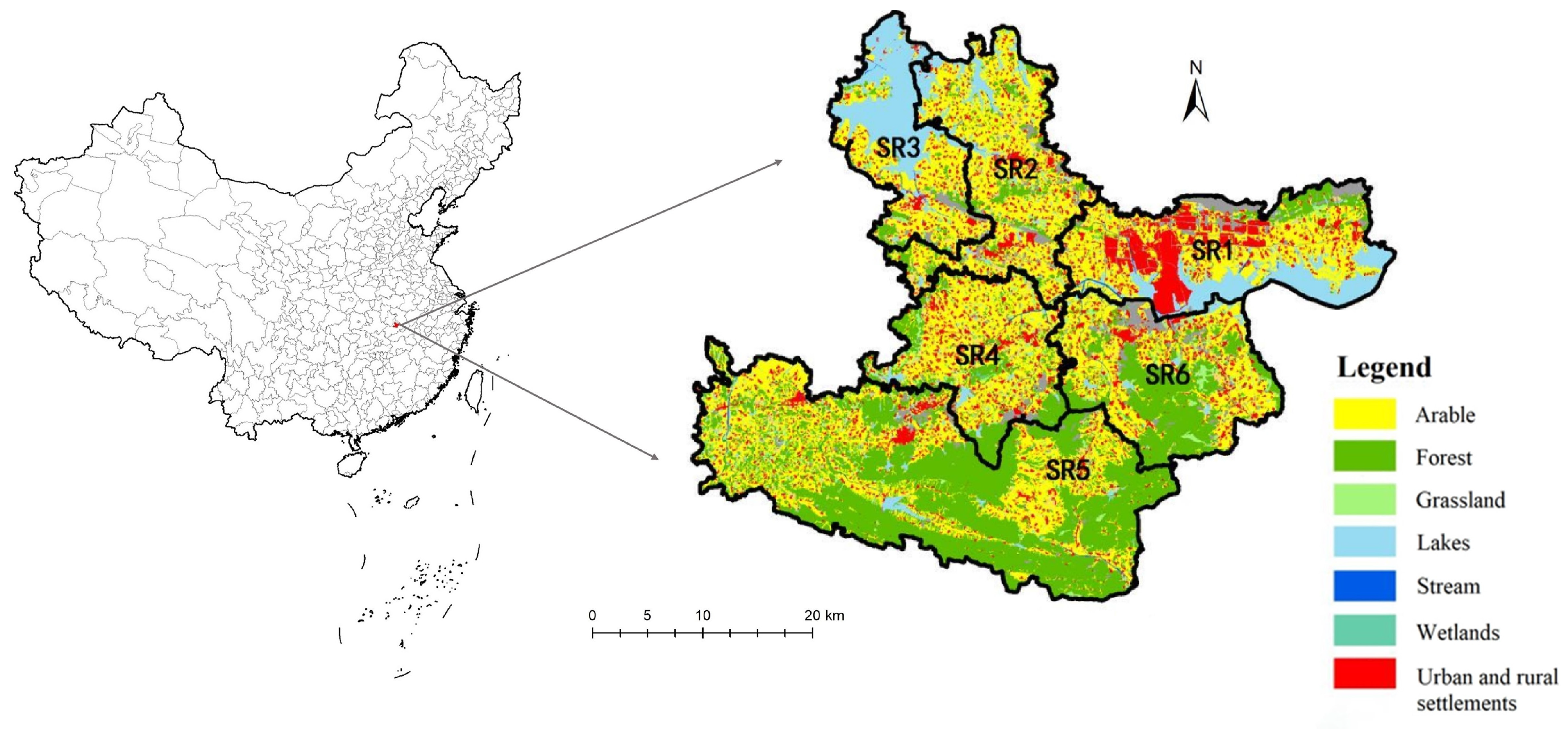
2.1. Study Area

Daye City is located in the southeastern part of Hubei, China, situated between 114°31′ to 115°20′ east longitude and 29°40′ to 30°15′ north latitude. This region is renowned for its rich mineral deposits, boasting advanced mining and metallurgy industries. The area also features a complete urban and peripheral ecosystem comprising lakes, rivers, forests, arable land, and parks, as well as urban and rural residential areas, covering a total land area of 1566.3 square kilometers. However, the prolonged mining and metallurgical processing activities have severely damaged the local ecosystem. These activities have led to issues like soil heavy metal pollution, water contamination, a decline in cultivated land quality, and significant geological environmental challenges. Consequently, the ecosystem’s functionality has been compromised, necessitating urgent measures to protect and remediate land resources and the environment. The study area in the present research was divided into six sub-regions, labeled as SR1, SR2 … SR6 in Figure 1, based on their economic, ecological, and geographical features (the base of the subdivision was added to the Supplementary Material).

2.2. Calculation of Land Use Degree

To reflect the intensity of land development and utilization in the study area, the different land use types in the study area were first divided into 4 grades based on the degree of human use (

Table 1. Grading of land use degree.

Type	Unused Land Grade	Forest, Grassland, Water Land Grade	Agricultural Land Grade	Urban Settlement Land Grade
Land Use Type	Unused Land or Difficult-to-Use Land	Forest, Grassland, Water Area	Arable Land, Orchard, Artificial Grassland	Urban, Residential Area, Industrial and Mining Land, Transportation Land
Grading Index	1	2	3	4

Source: Liu Jiyuan, 1997.

) [30]. The land use degree in the study area was then obtained by summing the weighted products of the percentage of each grade of land use type and the grading index. The calculation formula is as follows:

$$LUD={\sum }_{i=1}^n{L}_i\times A_i$$

(1)

where LUD represents the degree index of land use, $L_i$ represents the grading index of land use degree for the land type i in the study area, $A_i$ represents the proportion of land type, and i represents the land type.

2.3. Comprehensive Risk Assessment Model

Based on a historical review and current analyses of land resource and environmental degradation in Daye City, we introduced the ecological risk assessment framework proposed by the United States Environmental Protection Agency [31,32]. Drawing upon the research achievements of relevant scholars in regional ecological risk assessment [33,34,35], we constructed a comprehensive multi-indicator risk assessment model. Furthermore, we established an indicator system for regional ecological risk assessment from the perspectives of risk sources, risk severity, and ecological vulnerability. The weights for these indicators were determined using the Analytic Hierarchy Process (AHP).

2.3.1. Risk Calculation

Presently, the conceptual model of ecological risk assessment mainly comprises two aspects. First, the comprehensive risk probability assessment, based on risk sources, which mainly quantitatively describes risk sources based on occurrence possibility, intensity, and range of natural disasters or human-induced hazards; second, the assessment is further based on the degree of ecological damages of the receptors [36,37]. The calculation model of risk assessment is characterized as:

$$R=P·D$$

(2)

where R is the regional ecological risk value, D is the potential degree of risk loss of the ecosystem, and P is the probability or intensity of regional risk source. The representation of such a risk characterization has been widely recognized and extended into multiple fields.

On the basis of the quantitative calculation, the ecological risk index of the researched area is characterized through the following steps.

The probability of regional composite risk source, denoted by P, is calculated by the following equation:

$$P={\sum }_{j=1}^n{\sum }_{l=1}^m{\beta }_j{P}_{jl}$$

(3)

In Equation (3), $P_{jl}$ is the probability of the occurrence of l-grade, j-class ecological risks; ${\beta }_j$ is the weight of the j-th class ecological risks. Here, suppose there are n classes of risk sources for the object to be assessed, and this class of risk sources has m grades:

$${\sum }_{j=1}^n{\beta }_j=1$$

(4)

The ecological loss degree index represents the difference in ecological loss caused by each type of hazard, the vulnerability index denotes the vulnerability of different ecosystems, and the ecological index reflects the ecological significance and status of different ecosystems [38,39].

The potential hazard vulnerability of the researched area is calculated by:

$$D_i=W_i{E}_i+W_j{F}_i$$

(5)

In Equation (5), $D_i$ is the risk loss degree of biotope i in the region; $E_i$ is the ecological index in biotope i; and $F_i$ is the vulnerability of biotope i. $W_i$ and $W_j$ are weights of indicators.

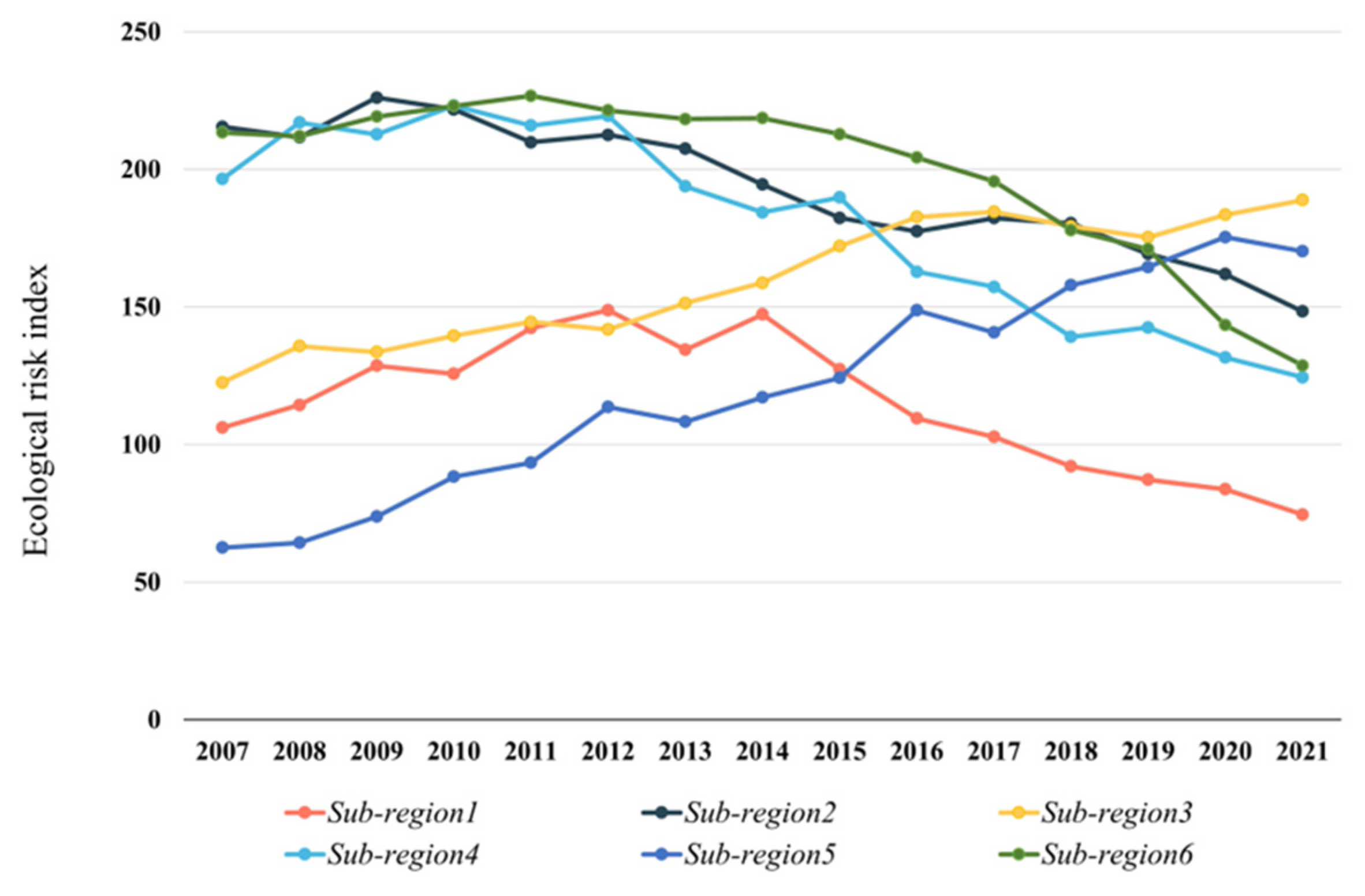
2.3.2. Analysis of the Ecological Risk in Study Area

This research was initiated based on damages to ecosystems. The formation of the problem is an important step toward determining the scope and purpose of the ecological risk assessment, which should cover all negative problems concerning different aspects of ecosystems. Whether ecological risk assessment itself and the subsequent management decision-making succeed relies on the quality of such a “problem formation” process. An arbitrary process of problem formation may cause a failure to accurately and comprehensively reflect the state of risks currently confronting the target system, and assessment on this basis would be valueless for risk managers [32,36]. Specifically, this process requires a range of work, from ecological endpoint determination to receptor selection, risk source identification and exposure-response analysis, to be completed in order to formulate an analytical plan and lay a foundation for the subsequent ecological risk assessment. The results of the risk investigation and variable determination are listed in the Supplementary Material.

(1)

Indicator system for regional ecological risk

Based on the assessment model, the hierarchal principle, and the principle of indicator system construction, an indicator system for regional ecological risk assessment was constructed from perspectives of the probability of composite risk sources and ecological vulnerability. Specifically, the ecological vulnerability indicator comprises the ecological quality index and the vulnerability index, and appropriate indicators were selected to quantify risks (Table 2). Data sources and processing were added to the Supplementary Materials (including both risk sources and ecological vulnerability).

Table 2. Index systems for ecological risks assessment.

System Layer	Variable Layer	Factor Layer	Index Layer	Observational Variable
Indicator system for regional ecological risks assessment	Probability of composite risk source	Probability of single risk	Refer to Table 3 for details
	Ecological vulnerability indicator (vulnerability)	Ecological quality index	Refer to Table 4 for details
		Vulnerability index

Table 2. Index systems for ecological risks assessment.

System Layer	Variable Layer	Factor Layer	Index Layer	Observational Variable
Indicator system for regional ecological risks assessment	Probability of composite risk source	Probability of single risk	Refer to Table 3 for details
	Ecological vulnerability indicator (vulnerability)	Ecological quality index	Refer to Table 4 for details
		Vulnerability index

Table 3. Ecological risk source weight distribution table.

Risk Source Type	Weight, %	Type	Weight, %	Ecological Risk Source	Weight, %
Natural disaster	0.2	Meteorological disaster	0.5	Storm flood	0.385
				Extreme weather	0.155
				Acid rain	0.46
		Geological disaster	0.5	Geological disaster	1
Human activity	0.8	Urban industrialization	0.559	Population aggregation	0.223
				The area ratio of industrial land	0.601
				Fixed investments (mining)	0.427
				Agricultural land reclamation	0.106
		Pollutant discharges	0.266	Point source	0.45
		Accumulation		Areal source	0.55
		Resource consumption and occupation	0.175	Agricultural irrigation	0.512
				Forest harvesting	0.38
				Grazing	0.108

Table 3. Ecological risk source weight distribution table.

Risk Source Type	Weight, %	Type	Weight, %	Ecological Risk Source	Weight, %
Natural disaster	0.2	Meteorological disaster	0.5	Storm flood	0.385
				Extreme weather	0.155
				Acid rain	0.46
		Geological disaster	0.5	Geological disaster	1
Human activity	0.8	Urban industrialization	0.559	Population aggregation	0.223
				The area ratio of industrial land	0.601
				Fixed investments (mining)	0.427
				Agricultural land reclamation	0.106
		Pollutant discharges	0.266	Point source	0.45
		Accumulation		Areal source	0.55
		Resource consumption and occupation	0.175	Agricultural irrigation	0.512
				Forest harvesting	0.38
				Grazing	0.108

Table 4. The index system of regional ecological vulnerability.

Object Layer	Factor Layer	Weight	Index Layer	Weight	Observational Variable	Weight
Ecological vulnerability degree	Ecological quality index	0.8	Natural biotope index (topography, geomorphology and climate)	0.135	Ground elevation	0.325
					Ratio of slope > 20 degrees to total area%	0.438
					Multi-year average precipitation	0.237
			Biotope index	0.259	Vegetation coverage	0.512
					Water network density	0.284
					Abundance of biological resources	0.204
			Vitality index	0.185	Ecological resilience value	0.415
					Primary productivity NPP	0.585
			Interreference index	0.192	Landscape fragmentation	0.632
					Shannon diversity index	0.368
			Environmental quality index	0.229	Water environment index	0.363
					Soil quality index	0.486
					Atmospheric index (fallout)	0.151
	Vulnerability index	0.2	Socioeconomic pressure index	1	Consumer price index (CPI)	0.381
					Fiscal income (GDP)	0.452

Table 4. The index system of regional ecological vulnerability.

Object Layer	Factor Layer	Weight	Index Layer	Weight	Observational Variable	Weight
Ecological vulnerability degree	Ecological quality index	0.8	Natural biotope index (topography, geomorphology and climate)	0.135	Ground elevation	0.325
					Ratio of slope > 20 degrees to total area%	0.438
					Multi-year average precipitation	0.237
			Biotope index	0.259	Vegetation coverage	0.512
					Water network density	0.284
					Abundance of biological resources	0.204
			Vitality index	0.185	Ecological resilience value	0.415
					Primary productivity NPP	0.585
			Interreference index	0.192	Landscape fragmentation	0.632
					Shannon diversity index	0.368
			Environmental quality index	0.229	Water environment index	0.363
					Soil quality index	0.486
					Atmospheric index (fallout)	0.151
	Vulnerability index	0.2	Socioeconomic pressure index	1	Consumer price index (CPI)	0.381
					Fiscal income (GDP)	0.452

(2)

Indicator system for hazardous degree assessment of the risk source

The hazardous degree of the risk source refers to different levels of risk stress confronting the structure, and the processes and functional bearing of the regional ecosystem caused by interferences from natural disasters and human activities. To establish risk source indicators, regional historical data and characteristics of development activities should be drawn upon to qualitatively and quantitatively analyze and predict potential ecological risks throughout their spatial distributions.

In this research, the hazardous degree of ecological risk sources comprises natural disasters and human activities, with the former including meteorological and geological disasters and the latter including urban industrialization, the accumulation of pollutant discharges, and the consumption and occupation of resources (Table 3).

Given the need to quantitatively calculate and spatially characterize different types of potential risk sources, it is necessary to analyze the weight of regional ecological risk sources of land. This research adopts the analytic hierarchy process (AHP) to determine the weights of indicators for the assessment of ecological risk sources. By comparing different pairs of indicators, a judgment matrix was established and a consistency test was calculated to determine the weight values of one sequence. A CR < 0.01 result on the consistency test given by the judgment matrix indicates that the weight is valid.

(3)

Indicator system for ecological vulnerability

Starting from the connotation of the vulnerability of the ecosystem itself, multiple rounds of discussions were organized to construct the indicator system for regional ecological vulnerability assessment from the perspectives of the ecological quality index and the vulnerability index (

Table 5. Unit root test for each sub-region.

Sub-Region	Variable	ADF Test	First Difference	Second Difference
1	Y1	−1.877	−4.143 ***	-
	X1	−1.056	−4.798 ***	-
2	Y2	−2.197	−3.259 +	-
	X2	−1.245	−7.042 ***	-
3	Y3	−1.734	−3.019	−4.505 ***
	X3	−2.214	−0.103	−6.643 ***
4	Y4	−3.662 *	-	-
	X4	−3.214 +	-	-
5	Y5	−4.827 ***	−6.607 ***	−8.654 ***
	X5	0.229	−2.039	−3.154 +
6	Y6	0.24	−7.13 ***	−8.928 ***
	X6	−0.035	−2.909	−3.276 +

*** p < 0.001, ** p < 0.01, * p < 0.05, ⁺ p < 0.1.

), with a view to reflecting the specific conditions of the land and the ecological vulnerability in Daye City. In the meantime, comparative judgment matrices were established to obtain the coefficients of weights of all indicators at different layers (Table 5). Based on the standardized values and weights of different factors in the assessment indicator system, the ecological vulnerability values of assessment units were obtained by weighted sum. The vulnerability takes a value between 0 and 1. The larger the value, the higher the ecological vulnerability, and vice versa.

2.4. Cointegration Analysis

Cointegration analysis is primarily employed to investigate long-term relationships among time series data, particularly when unit roots (non-stationarity) are present [40]. Through cointegration analysis, it is possible to delve deeper into issues related to the interactions and influence mechanisms among variables.

2.4.1. Unit Root Test

The ADF (Augmented Dickey–Fuller) test is a statistical method used to determine whether a given time series has a unit root (i.e., is not smooth). A unit root indicates that the time series data have some kind of trend or drift that makes them unsteady. The core objective of the ADF test is to test the null hypothesis that the time series data have a unit root (non-stationarity). If the results of the test reject the null hypothesis, then it can be concluded that the time series is smooth. The basic model of the ADF test is as follows:

$$∆y_t=\alpha +{\beta }_t+{\gamma y}_{\left\{t-1\right\}}+\Sigma {\phi }_i{∆y}_{\{t-1\}}+{\epsilon }_t$$

(6)

where $∆y_t$ represents the first-difference of the time series data, α is the constant term, ${\beta }_t$ is the time trend term, γ is the coefficient of $y_{\left\{t-1\right\}}$, ${\phi }_i$ is the coefficient of the lag term, and ${\epsilon }_t$ is the error term. In the ADF test, the parameters in the model are estimated and statistically tested to determine whether the coefficient γ is significantly non-zero. If γ is significantly non-zero, the null hypothesis is rejected and the series is considered stationary; if γ is not significantly non-zero, the null hypothesis cannot be rejected and the series is considered non-stationary.

2.4.2. Cointegration Test

Once the unit root characteristics of each variable are determined, the next step is to conduct cointegration tests to determine whether there exists a long-term stable relationship among these variables. The most commonly used cointegration tests are the Engle–Granger two-step method (E–G two-step method) and the Johansen multivariate cointegration test.

The E–G two-step method is a commonly used cointegration test method for determining whether there is a cointegration relationship between two time series variables [41]. Its basic steps and formulas are as follows:

• Regression Model Estimation

For two time series variables Y and X, we establish the linear regression model

$$Y_t=\alpha +{\beta X}_t+{\epsilon }_t$$

(7)

where $Y_t$ and $X_t$ represent the observations at time t, α is the intercept, β is the regression coefficient, and ${\epsilon }_t$ is the error term.

Estimate the parameters using the least squares method. Estimate the regression coefficients ${\alpha }_{hat}$ and ${\beta }_{hat}$ of the model using the least squares method.

2.

Residual Sequence Unit Root Test

Calculate the residual sequence $e_t$ using the estimated regression coefficients and observations

$$e_t=Y_t-{\alpha }_{hat} - {\beta }_{hat}\ast X_t$$

(8)

Perform a unit root test on the residual sequence, for example, using the ADF (Augmented Dickey–Fuller) test or the KPSS (Kwiatkowski–Phillips–Schmidt–Shin) test. These tests are used to determine whether the residual sequence is non-stationary. If the residual sequence passes the unit root test, i.e., it is determined to be stationary, it can be concluded that there exists a cointegration relationship between Y and X.

2.5. Granger Causality Test and Impulse Response Function

2.5.1. Granger Causality Test

The Granger causality test is a method used to test the relationship between time series data. The basic steps and related formulas for the Granger causality test are as follows.

Firstly, for two time series variables Y and X, we establish the following VAR models:

$$Y_t={\alpha }_Y+\Sigma {\beta }_{Yi}{Y}_{\{t-i\}}+\Sigma {\beta }_{Xi}{X}_{\{t-i\}}+{\epsilon }_{Yt}$$

(9)

$$X_t={\alpha }_X+\Sigma {\beta }_{Xi}{X}_{\{t-i\}}+\Sigma {\beta }_{Yi}{Y}_{\{t-i\}}+{\epsilon }_{Xt }$$

(10)

where $Y_t$ and $X_t$ represent the observed values at time t, ${\alpha }_Y$ and ${\alpha }_X$ are intercept terms, ${\beta }_{Yi}$ and ${\beta }_{Xi}$ are the corresponding coefficients, and ${\epsilon }_{Yt}$ and ${\epsilon }_{Xt}$ are the error terms.

Afterwards, the vector autoregressive (VAR) model is estimated using either the least squares method or maximum likelihood estimation to obtain estimates of the regression coefficients. Subsequently, tests such as the Ljung–Box test or the Durbin–Watson statistic are employed to examine whether the residual terms of the model form a white noise sequence. Finally, the Granger causality between the two variables is assessed by comparing the variances of the error terms in the two VAR models:

Null hypothesis (H0)—Y is not a Granger cause of X (i.e., X does not cause Y);

Alternative hypothesis (H1)—Y is a Granger cause of X (i.e., X causes Y).

The test statistic for the Granger causality test is the F-statistic, calculated as:

$$F=\frac{{RSS}_R-{RSS}_U}{q}/\frac{{RSS}_U}{n-k-1}$$

(11)

where ${RSS}_R$ is the residual sum of squares for the restricted model (assuming H0 is true), ${RSS}_U$ is the residual sum of squares for the unrestricted model (assuming H1 is true), q is the number of constraints (degrees of freedom for the restricted model), n is the sample size, and k is the total number of parameters in the model.

By comparing it with critical values and considering the statistical significance level, one can determine whether to reject the null hypothesis, thus assessing the presence of Granger causality between variables.

2.5.2. Impulse Response Function

The Impulse Response Function (IRF) is a method used to measure the dynamic relationship between time series variables [42]. It describes the impact of a shock (impulse) of a variable on other variables and its variation over time. The basic description and related formulas for IRF are as follows.

The calculation of IRF is based on the VAR model. For a p-order VAR model, it is represented as:

$$Y_t=\alpha +{\Sigma \phi }_i{Y}_{\{t-i\}}+{\epsilon }_t$$

(12)

where $Y_t$ is a k-dimensional time series vector, α is the intercept term, ${\phi }_i$ is the coefficient matrix for p lag orders, and ${\epsilon }_t$ is the residual term.

The IRF is calculated by simulating the application of a unit shock (impulse) to one variable and observing the dynamic response of other variables. Step 1 is selecting a variable as the impulse variable and applying a unit impulse at time t, represented as ${\epsilon }_t$ = [0, 0, …, 1, 0, 0]^T.

We then calculate the dynamic response. We introduce the impulse variable into the VAR model to obtain the dynamic response sequence of the VAR process. The dynamic response function is usually obtained through iterative calculations.

$${IRF}_{\left\{j,t\right\}}\left(h\right)={\phi }_{\{j,1\}}h{\epsilon }_h$$

(13)

where ${IRF}_{\left\{j,t\right\}}\left(h\right)$ represents the response of the j-th variable to the impulse variable at time t, ${\phi }_{\{j,1\}}h$ represents the dynamic response of the j-th variable to the impulse variable at time h, and ${\epsilon }_h$ represents the error term with an impulse applied at time h.

3. Results

3.1. Descriptive Statistics

According to the calculations, the land use degree index (Figure 2) and the ecological risk index (Figure 3) for Daye City from 2008 to 2021 were obtained. Observing the land use degree index chart, it can be noted that over the study period, the LUD in all six sub-regions shows an overall upward trend. However, the rate of increase tends to level off in the later years, indicating that there was significant development intensity in the early stages, and later land development and use became more rational. Specifically, Sub-region 1 stands out with the highest LUD, and it appears to have a significantly higher level of development compared to the other sub-regions, while Sub-region 5 exhibits a relatively lower land use degree.

In contrast, the ecological risk index does not exhibit a clear overall pattern. Over the period from 2007 to 2021, the ecological risk indices in Sub-regions 2, 4, and 6 show an overall decreasing trend. Conversely, Sub-regions 3 and 5 exhibit an overall increasing trend, while Sub-region 1 initially shows an increase followed by a decrease. Despite Sub-region 1 having the highest land use degree index, its ecological risk is the lowest in 2021.

3.2. Land Use and Ecological Risk Causality Tests

3.2.1. Unit Root Test

Based on the ecological risk index and land use degree from 2007 to 2021 in six sub-regions, the ADF test was conducted to test their stationarity. The test results for each sub-region are shown in Table 1. Based on the original values and the test results of the difference values, it can be seen that Y1 and X1 cannot reject the null hypothesis at a significance level of 5%, indicating that both are non-stationary series. However, the first differenced variables can reject the null hypothesis at a 0.1% significance level, indicating that both have no unit root in the first difference and are stationary series. Therefore, Y1 and X1 are first-order integrated sequences.

Similarly, it can be observed that Sub-region 4 exhibits a unit root process, Sub-region 2 follows a first-order integrated process, and Sub-regions 3, 5, and 6 display characteristics of a second-order integrated process. This finding suggests that, over the study period, the land utilization and regional ecological risk data in all six sub-regions maintain stationarity and exhibit mutual interactions.

3.2.2. Cointegration Test

The unit root tests indicate that both variables Y and X are integrations of order one within different sub-regions, suggesting the presence of a long-term stable relationship between them, whereby they co-evolve over the long run. To validate this hypothesis, the Engle–Granger two-step method can be employed to test whether there is cointegration between them.

According to the results of the Engle–Granger two-step test, as shown in

Table 6. E–G cointegration results for each region.

Sub-Region	Z-Value	Existence of Long-Term Stable Relationship
1	−3.546 **	Yes
2	−4.612 ***	Yes
3	−2.648 +	Yes
4	−3.413 **	Yes
5	−3.665 **	Yes
6	−4.129 ***	Yes

*** p < 0.001, ** p < 0.01, * p < 0.05, ⁺ p < 0.1.

, all six sub-regions passed the cointegration test. This implies the existence of a long-term equilibrium relationship between land utilization and ecological risk within these regions. The increase in land use degree has led to changes in land use structure, profoundly affecting the natural, economic, and social environment, thereby promoting an increase in ecological risk.

3.2.3. Error Correction Model

Determining the optimal lag order is crucial in time series analysis, as selecting the appropriate lag order ensures a better fit of the model to the data. Too few lag terms may result in the model failing to capture the dynamic relationships within the time series data, while too many lag terms can lead to overfitting, increasing model complexity, and reducing interpretability. To identify the optimal lag order, we typically utilize various information criteria, such as AIC, BIC, HQIC, etc. By comparing these criteria, the optimal lag orders for each sub-region are determined. Specifically, for VAR models in Sub-regions 1 to 6, the optimal lag orders are 2, 2, 3, 1, 1, and 2, respectively.

Furthermore, by generating stability plots (eigenvalue plots), the stability of VAR (vector autoregressive model) models in each region at the optimal lag order can be further examined. In an eigenvalue plot, the horizontal axis represents the index of eigenvalues, while the vertical axis represents the values of eigenvalues. If all eigenvalues are located within the unit circle (absolute values less than 1), it indicates that the model is stable. If there are eigenvalues outside the unit circle (absolute values greater than 1), it suggests that the model is unstable, and a reconsideration of the lag order selection is needed.

Based on the eigenvalue stability plots for the VAR models in each region at the optimal lag order (Figure 4), it can be concluded that all models exhibit stability. This means that the chosen optimal lag orders are suitable for the VAR models in each region, and these models can effectively capture the dynamic relationships in the data, providing reliable analytical results.

3.2.4. Granger Causality Test

To further explore the Granger causality relationship between ecological risk and land utilization in different regions, the Granger causality test was conducted, and the results are shown in

Table 7. Granger causality test results for each region.

Null Hypothesis	Region	Lag Order	Chi-Square Statistics	p-Value	Conclusion
Land use is not a Granger cause of ecological risk Ecological risk is not a Granger cause of land use	1	2	11.122	0.004	Rejected
		2	1.6832	0.431	Not Rejected
	2	2	1.1358	0.567	Not Rejected
		2	2.7653	0.251	Not Rejected
	3	3	6.1706	0.104	Not Rejected
		3	435.15	0.000	Rejected
	4	1	10.383	0.001	Rejected
		1	14.411	0.000	Rejected
	5	1	0.37045	0.543	Not Rejected
		1	0.5538	0.457	Not Rejected
	6	3	7.5963	0.055	Rejected
		3	22.231	0.000	Rejected

.

In Sub-region 1, the null hypothesis “land use is not a Granger cause of ecological risk” was rejected at a 5% significance level, but the null hypothesis “ecological risk is not a Granger cause of land use” failed to be rejected. This indicates a one-way causality relationship whereby an increase in land use degree is the cause of an increase in the ecological risk index, while an increase in the ecological risk index is not the cause of an increase in the land use degree. Similar conclusions were drawn for Sub-regions 2 and 5, where no Granger causality relationship was found. In Sub-region 3, ecological risk was found to be the cause of land use, indicating a one-way causality. Sub-regions 4 and 6 showed a bidirectional causality relationship

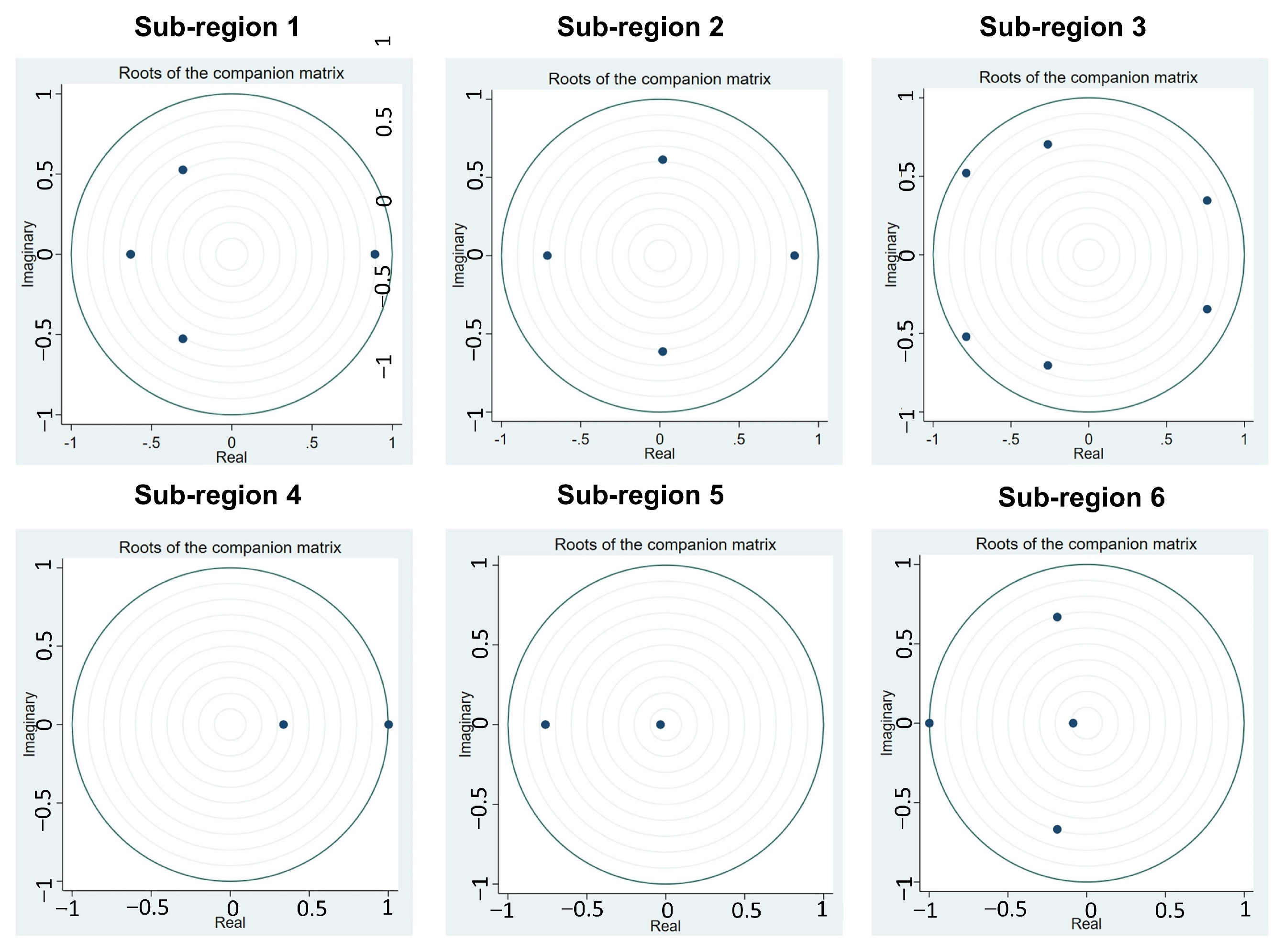
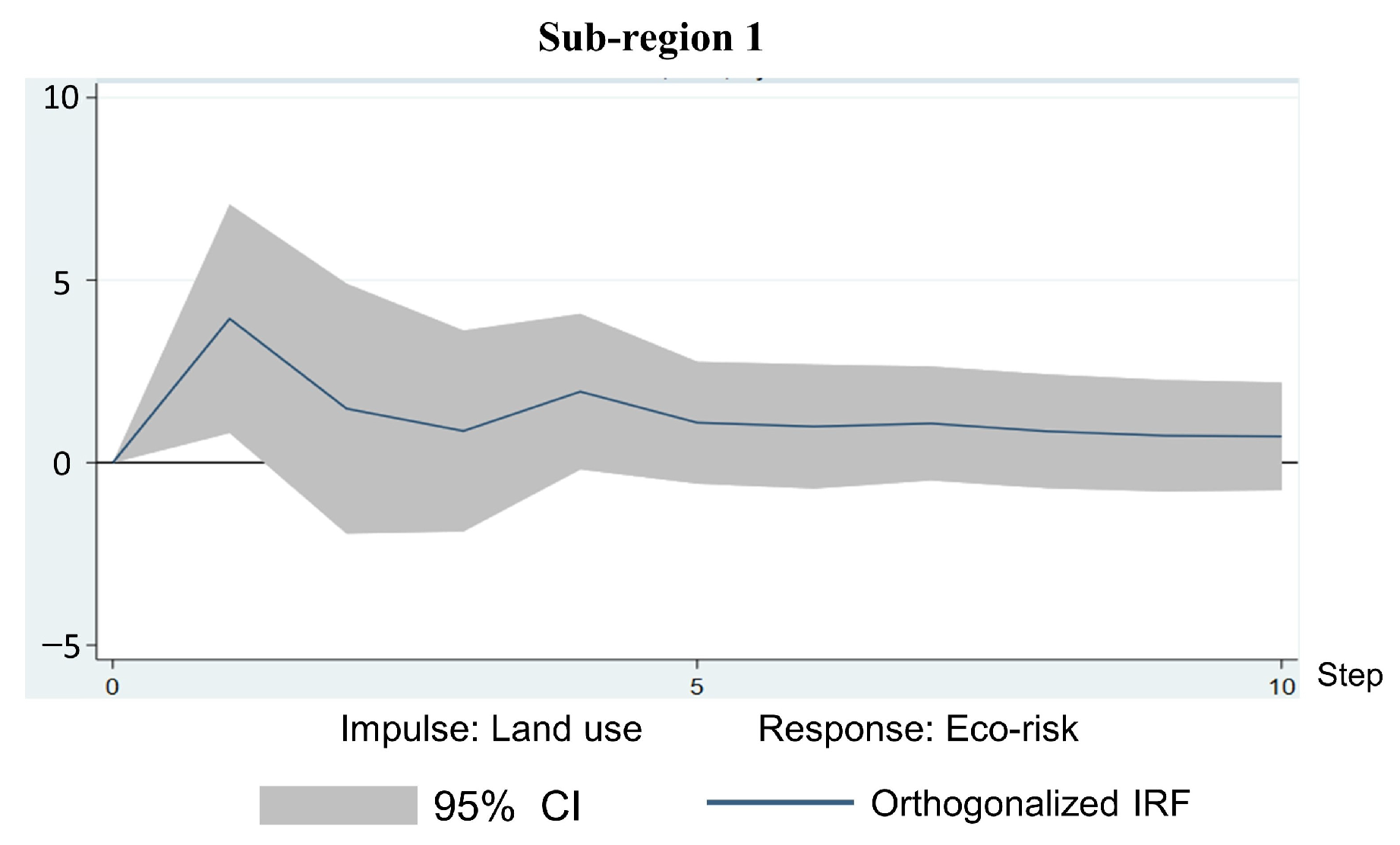
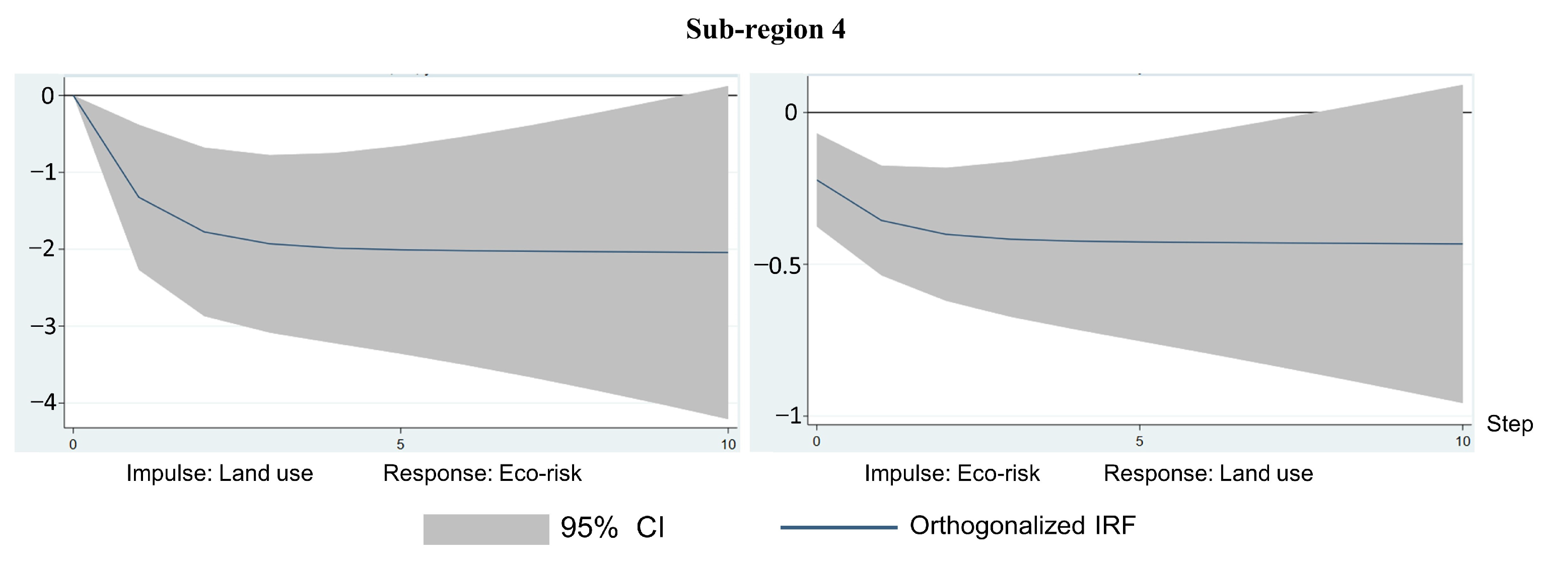
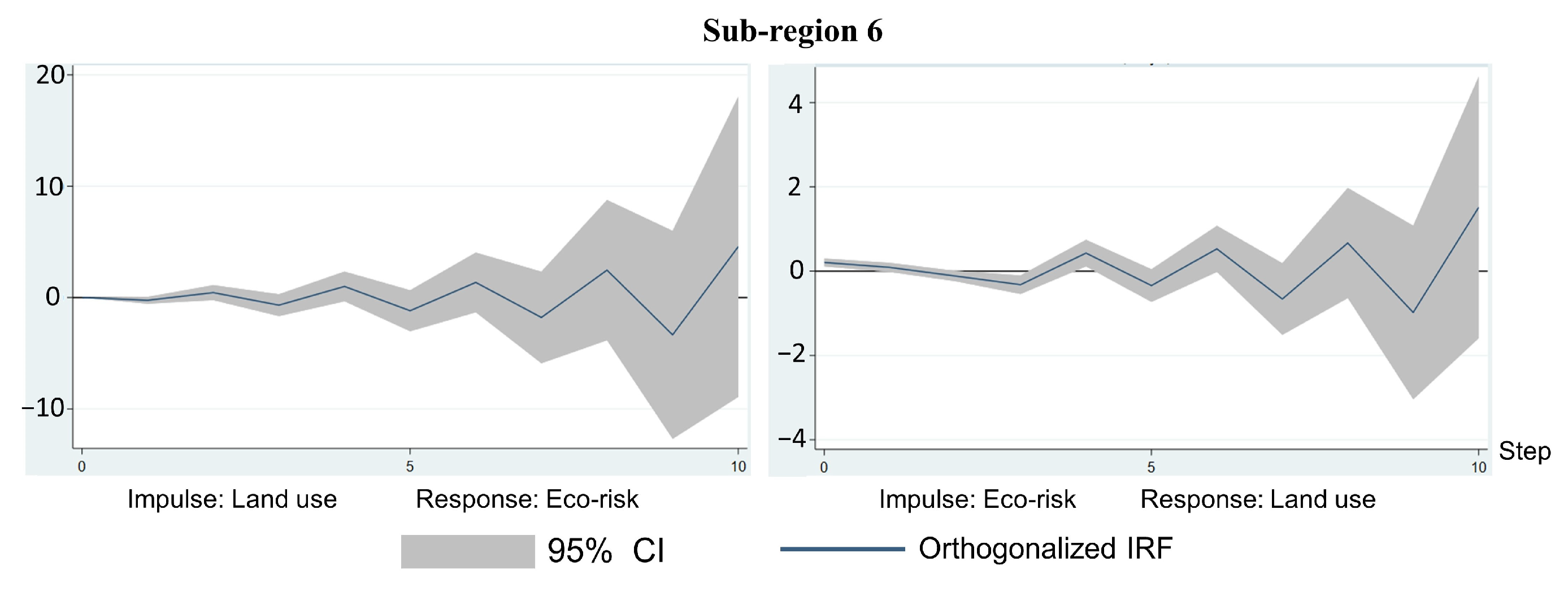
3.2.5. Impulse Response Analysis

Impulse response analysis can help reveal short-term impacts and interactions between variables. By analyzing impulse response functions, we can observe information such as the process of impact transmission between variables, the magnitude of responses, and their duration, thereby uncovering the dynamic relationships between variables. In the impulse response analysis graph, the 95% CI represents the confidence interval of the impulse response function, typically used to measure the range of uncertainty in the estimates. When the 95% CI includes the y = 0 line, it implies that the possibility of the impulse response function being equal to zero cannot be ruled out.

Based on the Granger causality test results, Figure 5, Figure 6, Figure 7 and Figure 8 displays the impulse response graphs for the selected regions. In Sub-region 1, the shock variable is land use, and the response variable is ecological risk. After giving a first-order shock to land use, the response of ecological risk is initially positive. However, as the number of periods increases, the positive response of ecological risk gradually decreases and eventually becomes statistically insignificant.

Based on Figure 6, in Sub-region 3, using ecological risk as the shock variable and land use as the response variable, the impact of ecological risk on land use fluctuates significantly. It is negative in the first period, insignificant in the second period, positive in the third period, and then becomes insignificant again. This fluctuation suggests that other more direct factors may be influencing changes in land use degree in this sub-region.

According to Figure 7, in Sub-region 4, the left graph shows land use as the shock variable and ecological risk as the response variable. It is evident that ecological risk exhibits a significant negative response to the changes in land use during the first two periods. However, in the subsequent periods, this impact gradually stabilizes. In the right graph, with ecological risk as the shock variable and land use degree as the response variable, similar to the previous scenario, ecological risk negatively affects land use, but the impact is relatively smaller compared to the former case. Moreover, this impact also tends to stabilize in the later periods.

From Figure 8, it can be noticed that in Sub-region 6, the left graph depicts land use as the shock variable and ecological risk as the response variable, while the right graph shows the reverse scenario. Overall, it can be observed that the impacts of mutual shocks between the two variables fluctuate considerably, and in most periods, they are statistically insignificant.

4. Discussion

4.1. Land Use and Ecological Risk Cointegration

Land use and ecological risk have been subjected to a cointegration test, revealing a long-term and stable relationship between them. This stability implies that over an extended period, these two variables do not exhibit persistent deviations. This can be attributed to various factors, including the adaptability of ecosystems to different land use practices and the implementation of sustainable approaches by land users. These sustainable practices encompass the effective planning and management of land use and ecological risks by the government, including environmental policies, regulations, and measures. Additionally, they involve the execution of land regeneration and restoration plans, water resource management, and pollution control, all contributing to the relative stability of land use and ecosystems.

4.2. Granger Causality Analysis for Different Sub-Regions

Land use in Sub-region 1 is identified as a key driver of ecological risk. This suggests that changes in land use may have a direct or indirect impact on the ecosystem, thereby increasing the potential for ecological risks. As an economic center and industrial hub, this region has undergone rapid urbanization over many years, resulting in the loss of critical habitats such as forests, lakes, wetlands, and grasslands. The decline in habitat diversity has significantly reduced the ecosystem’s resilience. Furthermore, the substantial population growth in tandem with the expansion of urban construction land may exacerbate the urban heat island effect. It is imperative for the government to prioritize thoughtful urban planning, optimize industrial structures, and continually enhance urban land utilization, all while rigorously controlling the proportion of construction land.

In Sub-region 3, ecological risk acts as the Granger cause of land use. This implies that the risk processes within the ecosystem have direct or indirect negative impacts on regional land use. Located in the northwest part, Sub-region 3 encompasses Daye City’s largest water body, Baoan Lake. Extensive aquaculture activities surrounding the lake have resulted in severe water pollution, particularly due to the application of agricultural feed, leading to water eutrophication. The overall degradation of the lake habitat has also impeded the rational use of land resources, including delays in tourism and wetland park development plans. Furthermore, to facilitate ecological recovery and preserve biodiversity, the government has imposed significant restrictions on the development of lake and wetland habitats.

In Sub-regions 4 and 6, there exists a bidirectional Granger causality relationship between land use and ecological risk. This mutual causality reflects the intricate and interconnected nature of land use and ecological risk. Sub-region 4 serves as an industrial hub for ore processing, encompassing activities such as ore beneficiation, washing, metallurgy, and handling. Not only does this sector encroach upon and waste significant land resources, it also contributes to deteriorating environmental conditions and health hazards in the vicinity. Large heaps of mining waste occupy vast spatial areas, placing the regional ecosystem in a prolonged state of high risk and impeding the rational utilization of land resources.

Sub-region 6, on the other hand, is a traditional copper mining area with a long history of elevated soil copper concentrations, posing a persistent challenge. The agricultural land, orchards, water bodies, and abandoned residential areas affected by heavy metal copper pollution remain idle or under strict usage restrictions. The high ecological risk associated with resource and environmental exploitation is a critical factor contributing to the stagnation of land use changes in these areas. Moreover, the complex and costly nature of soil heavy metal pollution remediation necessitates substantial government investment and long-term ecological restoration plans. Consequently, extensive habitats in these regions will continue to pose significant safety hazards and remain undeveloped for an extended period.

Sub-regions 2 and 5 do not exhibit a Granger causality between land use and ecological risks. Granger causality analysis indicates that when no Granger causality exists between land use and ecological risks, several possible explanations may be considered, including the variables being independent of each other, having only short-term relationships, involving complex causal pathways, being influenced by common factors, or being constrained by data limitations. To better understand this, we can analyze specific economic activities in these regions.

Sub-region 2, as a traditional iron and coal mining area, has long experienced frequent geological hazards such as “subsidence, collapse, landslides, and mudslides”. However, the ecological resettlement of mining area residents has already taken place, addressing the issue of ecological refugees as a whole. Moreover, the extensive land surface damage requires a long-term and complex land reclamation and restoration project, with planning, design, and funding still in the proposal stage. Therefore, we believe that in the time series under study, there is no discernible impact on land use and ecological risks in this sub-region.

Sub-region 5 in the southern part is a traditional agricultural and forestry management area, serving as a primary grain and timber production region in Daye City. The extensive use of pesticides, fertilizers, and plastic film has made it a high-risk area for organic pollution. Additionally, in pursuit of increased grain production, intensive farming practices have led to significant soil nutrient depletion and an increased risk of soil degradation. However, over the years, the government’s efforts to protect the forested areas, coupled with subsidies for forestry planting and guidance for farmers to explore alternative economic development models, have effectively prevented widespread forest degradation. Furthermore, the slow pace of urbanization and industrialization in the agricultural and forestry crop zones has resulted in relatively modest land cover changes. Therefore, in the experiment, it is possible that the two variables are relatively independent. Nevertheless, there could be other factors that are unaccounted for, such as climate change and population migration, which might simultaneously influence both land use and ecological risks

4.3. Land Use and Ecological Risk Pulse Analysis

It is important to note that while there is a cointegration relationship, it does not imply the absence of any issues or challenges between land use and ecological risk. It merely indicates a long-term trend of equilibrium between them, but short-term fluctuations and issues may still exist. The short-term fluctuations in land use and their influence on ecological risks typically result from the interplay of various factors. Firstly, land use can be susceptible to seasonal or cyclical influences, leading to short-term fluctuations. For instance, mining activities often coincide with specific seasons or cyclical peaks, exerting short-term pressures on ecosystems. Secondly, land use actions may trigger temporary disruptions within ecosystems, such as land reclamation, construction projects, and factory relocations. While these disruptions can briefly stress ecosystems, they may gradually return to a more stable state over time.

Furthermore, alterations in government policies and regulations, including changes in emission standards, mining taxation policies, water resource management policies, ecological refugee migrations, and fallow land policies, can also induce short-term variations in land use. Additionally, given that the mining industry serves as a pivotal economic pillar in Daye City, short-term fluctuations in land use can be influenced by market demands and price fluctuations within the mining sector. To comprehensively grasp the short-term impacts on ecosystems, it is essential to conduct an exhaustive examination of the relationship between land use and ecological risks within the study area.

5. Conclusions

This study used RRA and Granger causality analysis to jointly explore the relationship between land use and ecological risk in different regions of Daye City, a traditional industrial and mining city. The results show that (i) there is a significant long-term and stable relationship between changes in land use and ecological risk and (ii) due to regional differences, the Granger causality between land use and ecological security varies in different sub-regions. The combination of the results of this study and the understanding of the regional context will help regional decision-makers to make better judgements about the future land use structure, spatial layout, and use, and create better conditions for improving ecological security.

However, like any research, this study has certain shortcomings. Firstly, Granger causality analysis can only determine whether there is a “Granger causality” between variables, and the real causal mechanism analysis needs to exclude or control the influence of common factors and confounding variables; secondly, the construction of ecological security indicators involves more aspects, and the ecological risk indicator system constructed in this study may still be deficient. In future studies, methods such as machine learning can be further introduced to gain a deeper understanding of the potential causal mechanisms between land use and ecological risk, and provide valuable insights and suggestions for future regional development and planning.

References

1. McDowell, N.G.; Allen, C.D.; Anderson-Teixeira, K.; Aukema, B.H.; Bond-Lamberty, B.; Chini, L.; Clark, J.S.; Dietze, M.; Grossiord, C.; Hanbury-Brown, A.; et al. Pervasive Shifts in Forest Dynamics in a Changing World. Science 2020, 368, eaaz9463. [Google Scholar] [CrossRef]
2. Jin, X.; Jin, Y.; Mao, X. Ecological Risk Assessment of Cities on the Tibetan Plateau Based on Land Use/Land Cover Changes–Case Study of Delingha City. Ecol. Indic. 2019, 101, 185–191. [Google Scholar] [CrossRef]
3. Powers, R.P.; Jetz, W. Global Habitat Loss and Extinction Risk of Terrestrial Vertebrates under Future Land-Use-Change Scenarios. Nat. Clim. Chang. 2019, 9, 323–329. [Google Scholar] [CrossRef]
4. Kindu, M.; Schneider, T.; Teketay, D.; Knoke, T. Changes of Ecosystem Service Values in Response to Land Use/Land Cover Dynamics in Munessa–Shashemene Landscape of the Ethiopian Highlands. Sci. Total Environ. 2016, 547, 137–147. [Google Scholar] [CrossRef] [PubMed]
5. Liao, N.; Gu, X.; Wang, Y.; Xu, H.; Fan, Z. Analyzing Macro-Level Ecological Change and Micro-Level Farmer Behavior in Manas River Basin, China. Land 2020, 9, 250. [Google Scholar] [CrossRef]
6. Hou, D.; O’Connor, D.; Nathanail, P.; Tian, L.; Ma, Y. Integrated Gis and Multivariate Statistical Analysis for Regional Scale Assessment of Heavy Metal Soil Contamination: A Critical Review. Environ. Pollut. 2017, 231, 1188–1200. [Google Scholar] [CrossRef]
7. Guo, X.; Fang, C. Integrated Land Use Change Related Carbon Source/Sink Examination in Jiangsu Province. Land 2021, 10, 1310. [Google Scholar] [CrossRef]
8. Khaledian, Y.; Kiani, F.; Ebrahimi, S.; Brevik, E.; Aitkenhead-Peterson, J. Assessment and Monitoring of Soil Degradation During Land Use Change Using Multivariate Analysis. Land Degrad. Dev. 2017, 28, 128–141. [Google Scholar] [CrossRef]
9. de Baan, L.; Alkemade, R.; Koellner, T. Land Use Impacts on Biodiversity in Lca: A Global Approach. Int. J. Life Cycle Assess. 2013, 18, 1216–1230. [Google Scholar] [CrossRef]
10. Peters, M.K.; Hemp, A.; Appelhans, T.; Becker, J.N.; Behler, C.; Classen, A.; Detsch, F.; Ensslin, A.; Ferger, S.W.; Frederiksen, S.B.; et al. Climate–Land-Use Interactions Shape Tropical Mountain Biodiversity and Ecosystem Functions. Nature 2019, 568, 88–92. [Google Scholar] [CrossRef]
11. Mahowald, N.M.; Randerson, J.T.; Lindsay, K.; Munoz, E.; Doney, S.C.; Lawrence, P.; Schlunegger, S.; Ward, D.S.; Lawrence, D.; Hoffman, F.M. Interactions between Land Use Change and Carbon Cycle Feedbacks. Glob. Biogeochem. Cycles 2017, 31, 96–113. [Google Scholar] [CrossRef]
12. Wang, X.; Wu, J.; Liu, Y.; Hai, X.; Shanguan, Z.; Deng, L. Driving Factors of Ecosystem Services and Their Spatiotemporal Change Assessment Based on Land Use Types in the Loess Plateau. J. Environ. Manag. 2022, 311, 114835. [Google Scholar] [CrossRef] [PubMed]
13. Meneses, B.M.; Reis, R.; Vale, M.J.; Saraiva, R. Land Use and Land Cover Changes in Zêzere Watershed (Portugal)--Water Quality Implications. Sci. Total. Environ. 2015, 527, 439–447. [Google Scholar] [CrossRef] [PubMed]
14. Smith, P.; House, J.; Bustamante, M.; Sobocká, J.; Harper, R.; Pan, G.-X.; West, P.; Clark, J.; Adhya, T.; Rumpel, C.; et al. Global Change Pressures on Soils from Land Use and Management. Glob. Chang. Biol. 2016, 22, 1008–1028. [Google Scholar] [CrossRef]
15. Feng, Y.; Yang, Q.; Tong, X.; Chen, L. Evaluating Land Ecological Security and Examining Its Relationships with Driving Factors Using Gis and Generalized Additive Model. Sci. Total Environ. 2018, 633, 1469–1479. [Google Scholar] [CrossRef]
16. Liu, L.; Zhou, D.; Chang, X.; Lin, Z. A New Grading System for Evaluating China’s Cultivated Land Quality. Land Degrad. Dev. 2020, 31, 1482–1501. [Google Scholar] [CrossRef]
17. Dormann, C.F.; Schweiger, O.; Augenstein, I.; Bailey, D.; Billeter, R.; De Blust, G.; DeFilippi, R.; Frenzel, M.; Hendrickx, F.; Herzog, F.; et al. Effects of Landscape Structure and Land-Use Intensity on Similarity of Plant and Animal Communities. Glob. Ecol. Biogeogr. 2007, 16, 774–787. [Google Scholar] [CrossRef]
18. Fan, J.; Wang, Y.; Zhou, Z.; Nanshan, Y.; Meng, J. Dynamic Ecological Risk Assessment and Management of Land Use in the Middle Reaches of the Heihe River Based on Landscape Patterns and Spatial Statistics. Sustainability 2016, 8, 536. [Google Scholar] [CrossRef]
19. Yang, Z.; Chen, Y.; Qian, Q.; Wu, Z.; Zheng, Z.; Huang, Q. The Coupling Relationship between Construction Land Expansion and High-Temperature Area Expansion in China’s Three Major Urban Agglomerations. Int. J. Remote Sens. 2019, 40, 6680–6699. [Google Scholar] [CrossRef]
20. Zhang, H.; Feng, Z.; Shen, C.; Li, Y.; Feng, Z.; Zeng, W.; Huang, G. Relationship between the Geographical Environment and the Forest Carbon Sink Capacity in China Based on an Individual-Tree Growth-Rate Model. Ecol. Indic. 2022, 138, 108814. [Google Scholar] [CrossRef]
21. Wang, Z.; Li, X.; Yueting, M.; Li, L.; Wang, X.; Lin, Q. Dynamic Simulation of Land Use Change and Assessment of Carbon Storage Based on Climate Change Scenarios at the City Level: A Case Study of Bortala, China. Ecol. Indic. 2022, 134, 108499. [Google Scholar] [CrossRef]
22. Hunsaker, C.T.; Graham, R.L.; Suter, G.W.; O’Neill, B.; Jackson, B.L.; Barnthouse, L.W. Regional Ecological Risk Assessment: Theory and Demonstration; Technical Report; Oak Ridge National Lab. (ORNL): Oak Ridge, TN, USA, 1989.
23. Xu, X.; Xu, L.; Yan, L.; Ma, L.; Lu, Y. Integrated Regional Ecological Risk Assessment of Multi-Ecosystems under Multi-Disasters: A Case Study of China. Environ. Earth Sci. 2015, 74, 747–758. [Google Scholar] [CrossRef]
24. Kang, P.; Chen, W.; Hou, Y.; Li, Y. Linking Ecosystem Services and Ecosystem Health to Ecological Risk Assessment: A Case Study of the Beijing-Tianjin-Hebei Urban Agglomeration. Sci. Total Environ. 2018, 636, 1442–1454. [Google Scholar] [CrossRef] [PubMed]
25. Pártl, A.; Vačkář, D.; Loučková, B.; Krkoška Lorencová, E. A Spatial Analysis of Integrated Risk: Vulnerability of Ecosystem Services Provisioning to Different Hazards in the Czech Republic. Nat. Hazards 2017, 89, 1185–1204. [Google Scholar] [CrossRef]
26. Li, H.; Zhang, X.; Zhang, Y.; Yang, X.; Zhang, K. Risk Assessment of Forest Landscape Degradation Using Bayesian Network Modeling in the Miyun Reservoir Catchment (China) with Emphasis on the Beijing–Tianjin Sandstorm Source Control Program. Land Degrad. Dev. 2018, 29, 3876–3885. [Google Scholar] [CrossRef]
27. Shahbaz, M.; Hye, Q.M.A.; Tiwari, A.K.; Leitão, N.C. Economic Growth, Energy Consumption, Financial Development, International Trade and Co2 Emissions in Indonesia. Renew. Sustain. Energy Rev. 2013, 25, 109–121. [Google Scholar] [CrossRef]
28. Gries, T.; Redlin, M.; Ugarte, J.E. Human-Induced Climate Change: The Impact of Land-Use Change. Theor. Appl. Climatol. 2019, 135, 1031–1044. [Google Scholar] [CrossRef]
29. Zhang, M.; Wang, J.; Zhang, Y.; Wang, J. Ecological Response of Land Use Change in a Large Opencast Coal Mine Area of China. Resour. Policy 2023, 82, 103551. [Google Scholar] [CrossRef]
30. LIU, J. Macro Survey and Dynamic Research on Remote Sensing of Resources and Environment in China; Press of University of Science and Technology of China: Hefei, China, 1996. [Google Scholar]
31. Norton, S.B.; Rodier, D.J.; van der Schalie, W.H.; Wood, W.P.; Slimak, M.W.; Gentile, J.H. A Framework for Ecological Risk Assessment at the Epa. Environ. Toxicol. Chem. 1992, 11, 1663–1672. [Google Scholar] [CrossRef]
32. Suter II, G.W. Ecological Risk Assessment; CRC Press: Boca Raton, FL, USA, 2016. [Google Scholar]
33. Xu, X.; Lin, H.; Fu, Z. Probe into the Method of Regional Ecological Risk Assessment—A Case Study of Wetland in the Yellow River Delta in China. J. Environ. Manag. 2004, 70, 253–262. [Google Scholar] [CrossRef]
34. Xu, X.; Yan, L.; Xu, L.; Lu, Y.; Ma, L. Ecological Risk Assessment of Natural Disasters in China. Beijing Daxue Xuebao (Ziran Kexue Ban)/Acta Sci. Nat. Univ. Pekin. 2011, 47, 901–908. [Google Scholar]
35. Zhang, F.; Yushanjiang, A.; Wang, D. Ecological Risk Assessment Due to Land Use/Cover Changes (Lucc) in Jinghe County, Xinjiang, China from 1990 to 2014 Based on Landscape Patterns and Spatial Statistics. Environ. Earth Sci. 2018, 77, 491. [Google Scholar] [CrossRef]
36. Assessment, E.R. Guidelines for Ecological Risk Assessment; Environmental Protection Agency: Washington, DC, USA, 1998. [Google Scholar]
37. Guo, K.; Zhang, X.; Liu, J.; Wu, Z.; Chen, M.; Zhang, K.; Chen, Y. Establishment of an Integrated Decision-Making Method for Planning the Ecological Restoration of Terrestrial Ecosystems. Sci. Total Environ. 2020, 741, 139852. [Google Scholar] [CrossRef] [PubMed]
38. Iyalomhe, F.O.; Rizzi, J.; Pasini, S.; Torresan, S.; Critto, A.; Marcomini, A. Regional Risk Assessment for Climate Change Impacts on Coastal Aquifers. Sci. Total Environ. 2015, 537, 100–114. [Google Scholar] [CrossRef]
39. Clemens, M.; Khurelbaatar, G.; Merz, R.; Siebert, C.; van Afferden, M.; Rödiger, T. Groundwater Protection under Water Scarcity; from Regional Risk Assessment to Local Wastewater Treatment Solutions in Jordan. Sci. Total Environ. 2020, 706, 136066. [Google Scholar] [CrossRef]
40. Halicioglu, F. An Econometric Study of Co2 Emissions, Energy Consumption, Income and Foreign Trade in Turkey. Energy Policy 2009, 37, 1156–1164. [Google Scholar] [CrossRef]
41. Gil-Alana, L.A. Testing of Fractional Cointegration in Macroeconomic Time Series*. Oxf. Bull. Econ. Stat. 2003, 65, 517–529. [Google Scholar] [CrossRef]
42. Inoue, A.; Kilian, L. Joint Bayesian Inference About Impulse Responses in Var Models. J. Econom. 2022, 231, 457–476. [Google Scholar] [CrossRef]
Figure 1. Schematic diagram of the scope and geographical location of the study area.
Land 12 02060 g001
Figure 2. Land use degree index.
Land 12 02060 g002
Figure 3. Ecological risk index.
Land 12 02060 g003
Figure 4. Characteristic root test of VAR models for each region.
Land 12 02060 g004
Figure 5. Sub-region 1 impulse response.
Land 12 02060 g005
Figure 6. Sub-region 3 impulse response.
Land 12 02060 g006
Figure 7. Sub-region 4 impulse response.
Land 12 02060 g007
Figure 8. Sub-region 6 impulse response.
Land 12 02060 g008