


Spatiotemporal Characteristics and Influencing Factors of Urban Heat Island Based on Geographically Weighted Regression Model: A Case Study of Urumqi City

Abstract
:1. Introduction
2. Materials and Methods
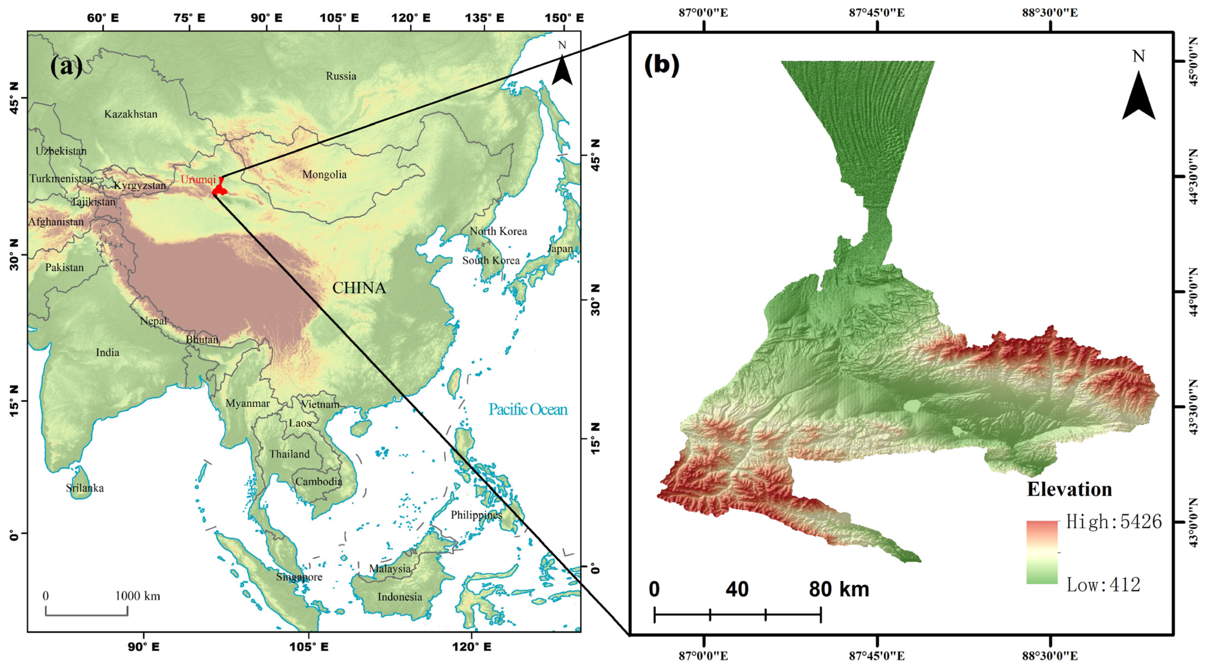
2.1. Study Area
2.2. Data Sources
2.3. Data Processing
2.3.1. Data Pre-Processing
2.3.2. Retrieval of the LST
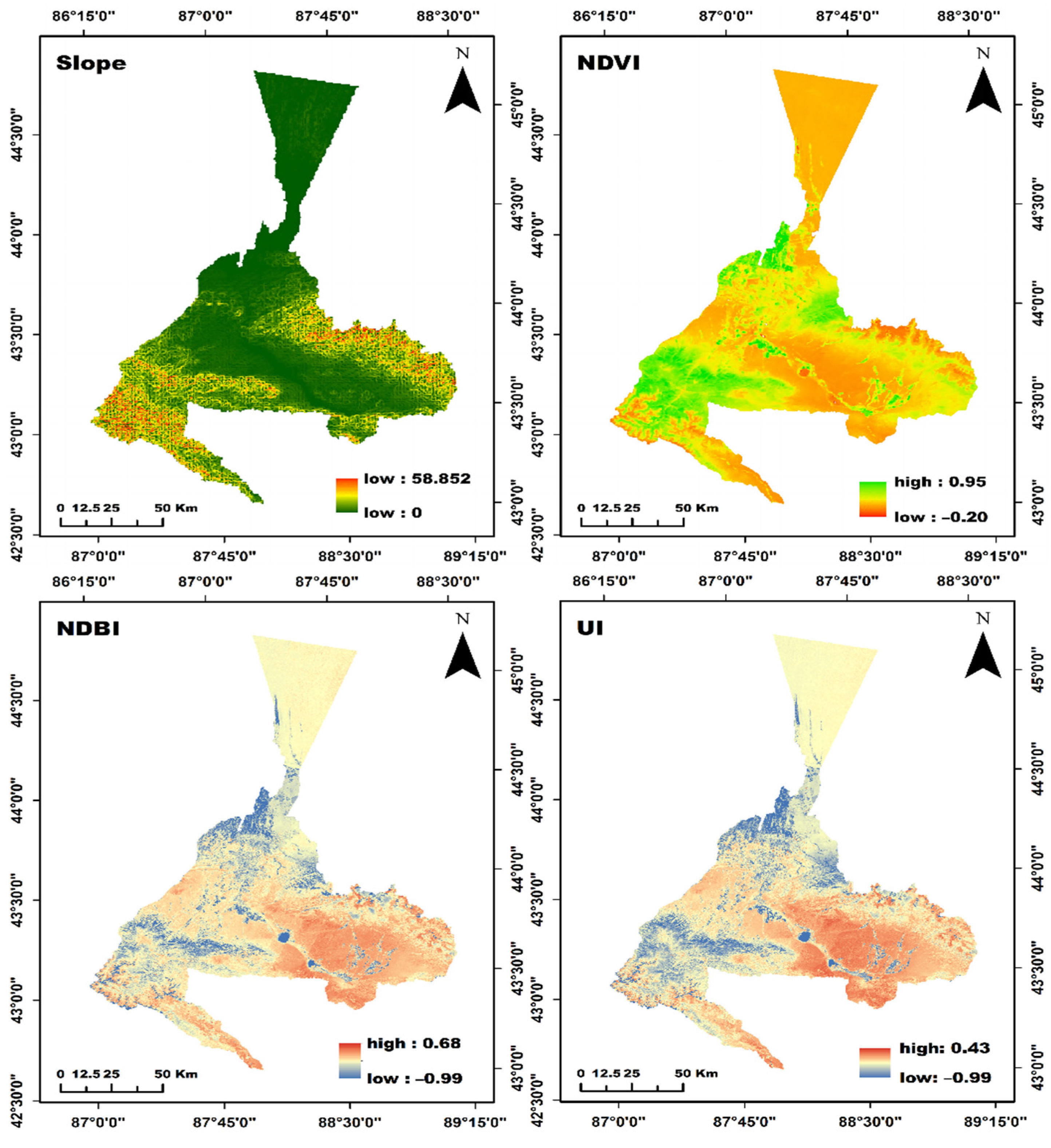
2.3.3. Selection and Calculation of the Influencing Factors
2.3.4. OLS and GWR Model
2.4. SUHI Intensity Classification
3. Results
3.1. The Spatiotemporal Characteristics of the LST
3.2. Analysis of Spatial and Temporal Variation in SUHII
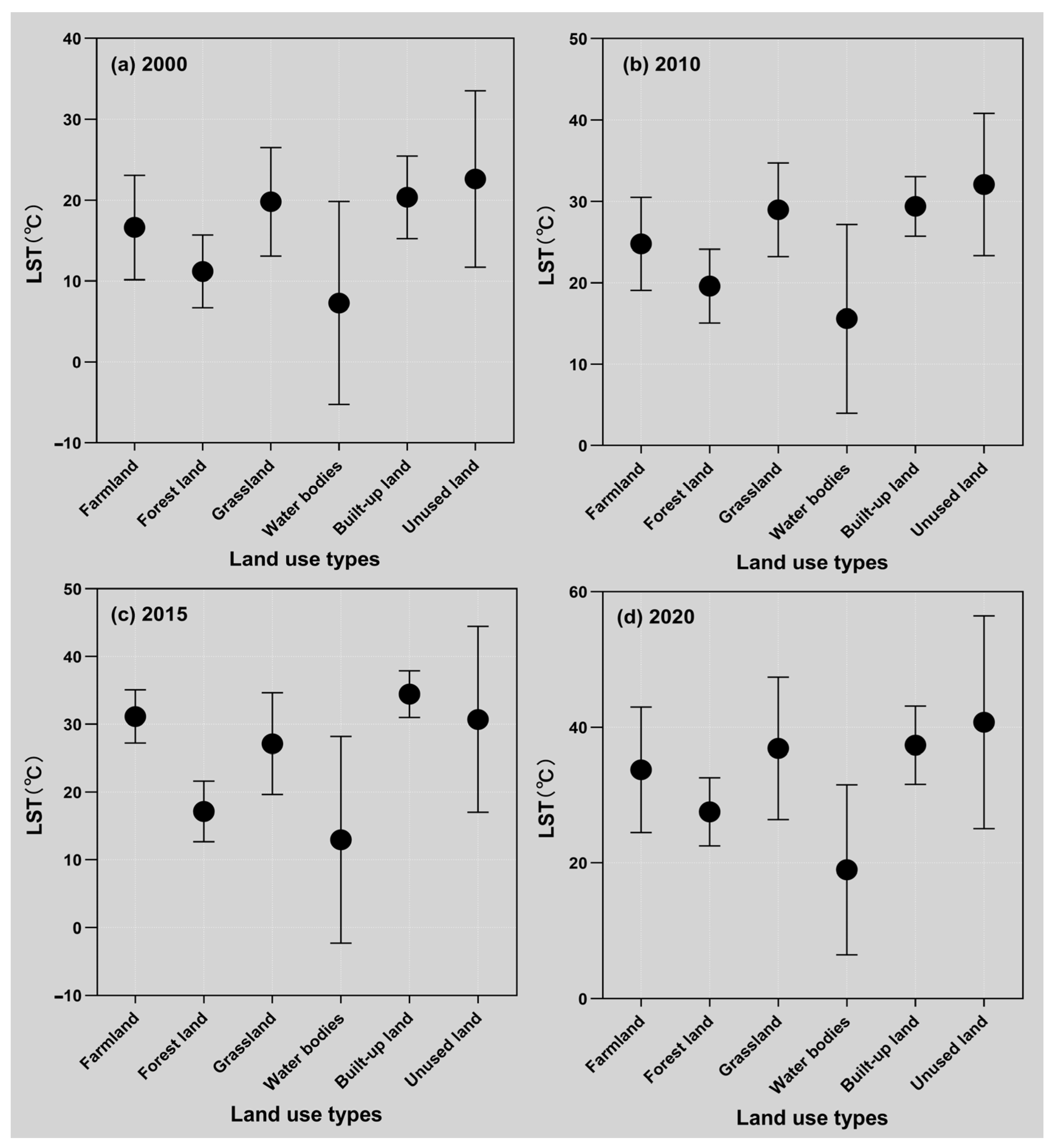
3.3. The Relationship between LULC and LST
3.4. Results of the OLS and GWR Model
4. Discussion
4.1. Analysis of the Relationship between LULC and LST
4.2. The Model Performance and Influencing Factors of SUHI
4.3. Limitations and Future Work
5. Conclusions
Author Contributions
Funding
Institutional Review Board Statement
Informed Consent Statement
Data Availability Statement
Acknowledgments
Conflicts of Interest
References
- Chen, M.; Lu, D.; Zha, L. The comprehensive evaluation of China’s urbanization and effects on resources and environment. J. Geogr. Sci. 2010, 20, 17–30. [Google Scholar] [CrossRef]
- Du, H.; Duoduo, W.; Wang, Y.; Zhao, X.; Qin, F.; Jiang, H.; Cai, Y. Influences of land cover types, meteorological conditions, anthropogenic heat and urban area on surface urban heat island in the Yangtze River Delta Urban Agglomeration. Sci. Total Environ. 2016, 571, 461–470. [Google Scholar] [CrossRef] [PubMed]
- He, W.; Li, X.; Yang, J.; Ni, H.; Sang, X. How land use functions evolve in the process of rapid urbanization: Evidence from Jiangsu Province, China. J. Clean. Prod. 2022, 380, 134877. [Google Scholar] [CrossRef]
- Uttara, S.; Bhuvandas, N.; Aggarwal, V. Impacts of urbanisation on environment. Int. J. Res. Eng. Appl. Sci. 2012, 2, 1637–1645. [Google Scholar]
- Gaffin, S.R.; Rosenzweig, C.; Khanbilvardi, R.; Parshall, L.; Mahani, S.; Glickman, H.; Goldberg, R.; Blake, R.; Slosberg, R.B.; Hillel, D. Variations in New York city’s urban heat island strength over time and space. Theor. Appl. Climatol. 2008, 94, 1–11. [Google Scholar] [CrossRef]
- Gunawardhana, L.N.; Kazama, S.; Kawagoe, S. Impact of Urbanization and Climate Change on Aquifer Thermal Regimes. Water Resour. Manag. 2011, 25, 3247–3276. [Google Scholar] [CrossRef]
- Liu, Y.; Yan, B.; Zhou, Y. Urbanization, economic growth, and carbon dioxide emissions in China: A panel cointegration and causality analysis. J. Geogr. Sci. 2016, 26, 131–152. [Google Scholar] [CrossRef]
- Jain, S.; Sannigrahi, S.; Sen, S.; Bhatt, S.; Chakraborti, S.; Rahmat, S. Urban heat island intensity and its mitigation strategies in the fast-growing urban area. J. Urban Manag. 2020, 9, 54–66. [Google Scholar] [CrossRef]
- Liu, K.; Li, X.; Wang, S.; Li, Y. Investigating the impacts of driving factors on urban heat islands in southern China from 2003 to 2015. J. Clean. Prod. 2020, 254, 120141. [Google Scholar] [CrossRef]
- Shi, Y.; Xiang, Y.; Zhang, Y. Urban Design Factors Influencing Surface Urban Heat Island in the High-Density City of Guangzhou Based on the Local Climate Zone. Sensors 2019, 19, 3459. [Google Scholar] [CrossRef]
- Sismanidis, P.; Bechtel, B.; Perry, M.; Ghent, D. The Seasonality of Surface Urban Heat Islands across Climates. Remote Sens. 2022, 14, 2318. [Google Scholar] [CrossRef]
- Wang, Y.; Yi, G.; Zhou, X.; Zhang, T.; Bie, X.; Li, J.; Ji, B. Spatial distribution and influencing factors on urban land surface temperature of twelve megacities in China from 2000 to 2017. Ecol. Indic. 2021, 125, 107533. [Google Scholar] [CrossRef]
- Manley, G. On the frequency of snowfall in metropolitan England. Q. J. R. Meteorol. Soc. 1958, 84, 70–72. [Google Scholar] [CrossRef]
- Yang, Y.; Guangrong, S.; Chen, Z.; Hao, S.; Zhouyiling, Z.; Shan, Y. Quantitative analysis and prediction of urban heat island intensity on urban-rural gradient: A case study of Shanghai. Sci. Total Environ. 2022, 829, 154264. [Google Scholar] [CrossRef] [PubMed]
- Li, F.-J.; Ma, A.-Q.; Ding, Y.-D.; Yang, J.-J.; Jiao, J.-C.; Liu, L.-J. Research on Urban Heat Island Effect Based on Landsat Data. Remote Sens. Technol. Appl. 2009, 24, 553–558. (In Chinese) [Google Scholar] [CrossRef]
- Liu, W.; Yang, P.; You, H.; Zhang, B. Heat Island Effect and Diurnal Temperature Range in Beijing Area. Clim. Environ. Res. 2013, 18, 171–177. (In Chinese) [Google Scholar] [CrossRef]
- Chen, Y.-C.; Chen, C.-Y.; Matzarakis, A.; Liu, J.-K.; Lin, T.-P. Modeling of mean radiant temperature based on comparison of airborne remote sensing data with surface measured data. Atmos. Res. 2016, 174–175, 151–159. [Google Scholar] [CrossRef]
- Abulibdeh, A. Analysis of urban heat island characteristics and mitigation strategies for eight arid and semi-arid gulf region cities. Environ. Earth Sci. 2021, 80, 259. [Google Scholar] [CrossRef]
- Chen, Y.; Weng, Q.H.; Tang, L.L.; Wang, L.; Xing, H.F.; Liu, Q.H. Developing an intelligent cloud attention network to support global urban green spaces mapping. ISPRS J. Photogramm. Remote Sens. 2023, 198, 197–209. [Google Scholar] [CrossRef]
- Liu, H.; Shen, G.; Huang, Q. Evolution of urban heat island effect and its relationship with land use change in wuhan city in recent 10 years. Resour. Environ. Yangtze Basin 2017, 26, 1466–1475. (In Chinese) [Google Scholar] [CrossRef]
- Sekertekin, A.; Bonafoni, S. Land Surface Temperature Retrieval from Landsat 5, 7, and 8 over Rural Areas: Assessment of Different Retrieval Algorithms and Emissivity Models and Toolbox Implementation. Remote Sens. 2020, 12, 294. [Google Scholar] [CrossRef]
- Silva, J.S.; da Silva, R.M.; Santos, C.A.G. Spatiotemporal impact of land use/land cover changes on urban heat islands: A case study of Paco do Lumiar, Brazil. Build. Environ. 2018, 136, 279–292. [Google Scholar] [CrossRef]
- Xu, X.; Pei, H.Y.; Wang, C.; Xu, Q.Y.; Xie, H.; Jin, Y.M.; Feng, Y.J.; Tong, X.H.; Xiao, C.J. Long-term analysis of the urban heat island effect using multisource Landsat images considering inter-class differences in land surface temperature products. Sci. Total Environ. 2023, 858, 159777. [Google Scholar] [CrossRef] [PubMed]
- Tesfamariam, S.; Govindu, V.; Uncha, A. Spatio-temporal analysis of urban heat island (UHI) and its effect on urban ecology: The case of Mekelle city, Northern Ethiopia. Heliyon 2023, 9, e13098. [Google Scholar] [CrossRef]
- Welegedara, N.P.Y.; Agrawal, S.K.; Lotfi, G. Exploring spatiotemporal changes of the urban heat Island effect in high-latitude cities at a neighbourhood level: A case of Edmonton, Canada. Sustain. Cities Soc. 2023, 90, 104403. [Google Scholar] [CrossRef]
- Rizwan, A.M.; Dennis, L.Y.C.; Liu, C. A review on the generation, determination and mitigation of Urban Heat Island. J. Environ. Sci. 2008, 20, 120–128. [Google Scholar] [CrossRef] [PubMed]
- Zhou, S.; Liu, D.; Zhu, M.; Tang, W.; Chi, Q.; Ye, S.; Xu, S.; Cui, Y. Temporal and Spatial Variation of Land Surface Temperature and Its Driving Factors in Zhengzhou City in China from 2005 to 2020. Remote Sens. 2022, 14, 4281. [Google Scholar] [CrossRef]
- Hung, T.; Uchihama, D.; Ochi, S.; Yasuoka, Y. Assessment with satellite data of the urban heat island effects in Asian mega cities. Int. J. Appl. Earth Obs. Geoinf. 2006, 8, 34–48. [Google Scholar] [CrossRef]
- Shahfahad; Bindajam, A.A.; Naikoo, M.W.; Horo, J.P.; Mallick, J.; Rihan, M.; Malcoti, M.D.; Talukdar, S.; Rahman, R.; Rahman, A. Response of soil moisture and vegetation conditions in seasonal variation of land surface temperature and surface urban heat island intensity in sub-tropical semi-arid cities. Theor. Appl. Climatol. 2023, 153, 367–395. [Google Scholar] [CrossRef]
- Enete, A.A.; Madu, I.A.; Onwubuya, E.A. Climate change and the profitability of indigenous adaptation practices in smallholder agriculture in South East Nigeria. Outlook Agric. 2012, 41, 179–185. [Google Scholar] [CrossRef]
- Zhang, C.; Xie, G.; Lu, C.; Liu, C.; Li, N.; Wang, S.; Sun, Y. The mitigating effects of different urban green lands on the heat island effect in Beijing. Resour. Sci. 2015, 37, 1156–1165. (In Chinese) [Google Scholar]
- Liu, Y.; Yuan, Z.; Kong, W.; Sun, B.; An, B. The Changing Trend of Heat Island Intensity and Main Influencing Factors during 1993–2012 in Xian City. J. Nat. Resour. 2015, 30, 974–985. (In Chinese) [Google Scholar] [CrossRef]
- Xiong, Y.; Zhang, F. Thermal environment effects of urban human settlements and influencing factors based on multi-source data: A case study of Changsha city. Acta Geogr. Sin. 2020, 75, 2443–2458. (In Chinese) [Google Scholar] [CrossRef]
- Zhao, C.H.; Jensen, J.; Weng, Q.H.; Weaver, R. A Geographically Weighted Regression Analysis of the Underlying Factors Related to the Surface Urban Heat Island Phenomenon. Remote Sens. 2018, 10, 1428. [Google Scholar] [CrossRef]
- Brunsdon, C.; Fotheringham, A.S.; Charlton, M. Some notes on parametric significance tests for geographically weighted regression. J. Reg. Sci. 1999, 39, 497–524. [Google Scholar] [CrossRef]
- Wang, J.; Qian, Y.-G.; Han, L.-J.; Zhou, W.-Q. Relationship between land surface temperature and land cover types based on GWR model: A case of Beijing-Tianjin-Tangshan urban agglomeration, China. Yingyong Shengtai Xuebao 2016, 27, 2128–2136. (In Chinese) [Google Scholar] [CrossRef] [PubMed]
- Kashki, A.; Karami, M.; Zandi, R.; Roki, Z. Evaluation of the effect of geographical parameters on the formation of the land surface temperature by applying OLS and GWR, A case study Shiraz City, Iran. Urban Clim. 2021, 37, 100832. [Google Scholar] [CrossRef]
- Li, L.; Zha, Y.; Zhang, J. Spatially non-stationary effect of underlying driving factors on surface urban heat islands in global major cities. Int. J. Appl. Earth Obs. Geoinf. 2020, 90, 102131. [Google Scholar] [CrossRef]
- Yu, Z.; Li, X.; Tursun, H. Research on Environmental Sustainability Degree in Urumqi. J. Arid. Land Resour. Environ. 2002, 16, 15–21. (In Chinese) [Google Scholar] [CrossRef]
- Alimjan, A.; Amanguli, S.; Hui, L.I.U.; Turangul, H. Population development trend of Urumqi in future. J. Arid. Land Resour. Environ. 2011, 25, 32–38. [Google Scholar] [CrossRef]
- Xuegang, C.; Zhaoping, Y. Study on Simulating Spatial Distribution and Varying Patterns of Population in Urumqi Based on GIS. J. Arid. Land Resour. Environ. 2008, 22, 12–16. (In Chinese) [Google Scholar] [CrossRef]
- Xu, H.Q. Retrieval of the reflectance and land surface temperature of the newly-launched Landsat 8 satellite. Chin. J. Geophys.-Chin. Ed. 2015, 58, 741–747. (In Chinese) [Google Scholar] [CrossRef]
- Sobrino, J.A.; Jiménez-Muñoz, J.C.; Paolini, L. Land surface temperature retrieval from LANDSAT TM 5. Remote Sens. Environ. 2004, 90, 434–440. [Google Scholar] [CrossRef]
- Dong, X.; Tian, J.; Zhang, R.H.; He, D.X.; Chen, Q.M. Study on the Relationship between Soil Emissivity Spectra and Content of Soil Elements. Spectrosc. Spectr. Anal. 2017, 37, 557–565. (In Chinese) [Google Scholar] [CrossRef]
- Seto, K.C.; Kaufmann, R.K. Modeling the drivers of urban land use change in the Pearl River Delta, China: Integrating remote sensing with socioeconomic data. Land Econ. 2003, 79, 106–121. [Google Scholar] [CrossRef]
- Hidalgo-García, D.; Arco-Díaz, J. Modeling the Surface Urban Heat Island (SUHI) to study of its relationship with variations in the thermal field and with the indices of land use in the metropolitan area of Granada (Spain). Sustain. Cities Soc. 2022, 87, 104166. [Google Scholar] [CrossRef]
- Wilson, J.S.; Clay, M.; Martin, E.; Stuckey, D.; Vedder-Risch, K. Evaluating environmental influences of zoning in urban ecosystems with remote sensing. Remote Sens. Environ. 2003, 86, 303–321. [Google Scholar] [CrossRef]
- Brunsdon, C.; Fotheringham, A.S.; Charlton, M.E. Geographically Weighted Regression: A Method for Exploring Spatial Nonstationarity. Geogr. Anal. 1996, 28, 281–298. [Google Scholar] [CrossRef]
- Md Bohari, N.F.; Kruger, E.; John, J.; Tennant, M. Analysis of dental services distribution in Malaysia: A geographic information systems—Based approach. Int. Dent. J. 2019, 69, 223–229. [Google Scholar] [CrossRef] [PubMed]
- Brunsdon, C.; Fotheringham, A.S.; Charlton, M. Geographically weighted summary statistics—A framework for localised exploratory data analysis. Comput. Environ. Urban Syst. 2002, 26, 501–524. [Google Scholar] [CrossRef]
- Guo, L.; Ma, Z.H.; Zhang, L.J. Comparison of bandwidth selection in application of geographically weighted regression: A case study. Can. J. For. Res. 2008, 38, 2526–2534. [Google Scholar] [CrossRef]
- Ünal, Y.S.; Sonuç, C.Y.; Incecik, S.; Topcu, H.S.; Diren-Üstün, D.H.; Temizöz, H.P. Investigating urban heat island intensity in Istanbul. Theor. Appl. Climatol. 2020, 139, 175–190. [Google Scholar] [CrossRef]
- Bechtel, B.; Demuzere, M.; Mills, G.; Zhan, W.; Sismanidis, P.; Small, C.; Voogt, J. SUHI analysis using Local Climate Zones—A comparison of 50 cities. Urban Clim. 2019, 28, 100451. [Google Scholar] [CrossRef]
- Shahfahad; Naikoo, M.W.; Towfiqul Islam, A.R.M.; Mallick, J.; Rahman, A. Land use/land cover change and its impact on surface urban heat island and urban thermal comfort in a metropolitan city. Urban Clim. 2022, 41, 101052. [Google Scholar] [CrossRef]
- Lu, L.; Weng, Q.; Xiao, D.; Guo, H.; Li, Q.; Hui, W. Spatiotemporal Variation of Surface Urban Heat Islands in Relation to Land Cover Composition and Configuration: A Multi-Scale Case Study of Xi’an, China. Remote Sens. 2020, 12, 2713. [Google Scholar] [CrossRef]
- Amindin, A.; Pouyan, S.; Pourghasemi, H.R.; Yousefi, S.; Tiefenbacher, J.P. Spatial and temporal analysis of urban heat island using Landsat satellite images. Environ. Sci. Pollut. Res. 2021, 28, 41439–41450. [Google Scholar] [CrossRef]
- Kaur, R.; Pandey, P. Spatial trends of surface urban heat island in Bathinda: A semiarid city of northwestern India. Int. J. Environ. Sci. Technol. 2022, 19, 10911–10932. [Google Scholar] [CrossRef]
- Song, J.; Du, S.; Feng, X.; Guo, L. The relationships between landscape compositions and land surface temperature: Quantifying their resolution sensitivity with spatial regression models. Landsc. Urban Plan. 2014, 123, 145–157. [Google Scholar] [CrossRef]
- Ma, X.L.; Peng, S.Y. Research on the spatiotemporal coupling relationships between land use/land cover compositions or patterns and the surface urban heat island effect. Environ. Sci. Pollut. Res. 2022, 29, 39723–39742. [Google Scholar] [CrossRef]
- Cai, Y.B.; Zhang, H.; Zheng, P.; Pan, W.B. Quantifying the Impact of Land use/Land Cover Changes on the Urban Heat Island: A Case Study of the Natural Wetlands Distribution Area of Fuzhou City, China. Wetlands 2016, 36, 285–298. [Google Scholar] [CrossRef]
- Saha, S.; Saha, A.; Das, M.; Saha, A.; Sarkar, R.; Das, A. Analyzing spatial relationship between land use/land cover (LULC) and land surface temperature (LST) of three urban agglomerations (UAs) of Eastern India. Remote Sens. Appl. Soc. Environ. 2021, 22, 100507. [Google Scholar] [CrossRef]
- Njoku, E.A.; Tenenbaum, D.E. Quantitative assessment of the relationship between land use/land cover (LULC), topographic elevation and land surface temperature (LST) in Ilorin, Nigeria. Remote Sens. Appl. Soc. Environ. 2022, 27, 100780. [Google Scholar] [CrossRef]
- Moisa, M.B.; Gemeda, D.O. Assessment of urban thermal field variance index and thermal comfort level of Addis Ababa metropolitan city, Ethiopia. Heliyon 2022, 8, e10185. [Google Scholar] [CrossRef]
- Weng, Q.H.; Lu, D.S.; Schubring, J. Estimation of land surface temperature-vegetation abundance relationship for urban heat island studies. Remote Sens. Environ. 2004, 89, 467–483. [Google Scholar] [CrossRef]
- Gao, Y.; Zhao, J.; Han, L. Exploring the spatial heterogeneity of urban heat island effect and its relationship to block morphology with the geographically weighted regression model. Sustain. Cities Soc. 2022, 76, 103431. [Google Scholar] [CrossRef]
- Anniballe, R.; Bonafoni, S.; Pichierri, M. Spatial and temporal trends of the surface and air heat island over Milan using MODIS data. Remote Sens. Environ. 2014, 150, 163–171. [Google Scholar] [CrossRef]
- Derdouri, A.; Murayama, Y.; Morimoto, T. Spatiotemporal Thermal Variations in Moroccan Cities: A Comparative Analysis. Sensors 2023, 23, 6229. [Google Scholar] [CrossRef] [PubMed]
- Shahfahad; Talukdar, S.; Rihan, M.; Hang, H.T.; Bhaskaran, S.; Rahman, A. Modelling urban heat island (UHI) and thermal field variation and their relationship with land use indices over Delhi and Mumbai metro cities. Environ. Dev. Sustain. 2022, 24, 3762–3790. [Google Scholar] [CrossRef]
- Chen, F.; Yang, S.; Yin, K.; Chan, P. Challenges to quantitative applications of Landsat observations for the urban thermal environment. J. Environ. Sci. 2017, 59, 80–88. [Google Scholar] [CrossRef]


| Years | Sensor | Path/Row | Acquisition Time | Cloud Cover |
|---|---|---|---|---|
| 2000 | Landsat-5 TM | 142/029 | 14 June 2000 (12:26:04) | 0.00 |
| 142/030 | 2 September 2000 (12:28:10) | 1.00 | ||
| 143/029 | 25 September 2000 (12:34:16) | 3.00 | ||
| 143/030 | 25 September 2000 (12:34:40) | 2.00 | ||
| 2010 | Landsat-5 TM | 142/029 | 13 August 2010 (12:40:04) | 0.01 |
| 142/030 | 13 August 2010 (12:40:29) | 0.03 | ||
| 143/029 | 20 August 2010 (12:46:14) | 0.00 | ||
| 143/030 | 20 August 2010 (12:46:38) | 6.36 | ||
| 2015 | Landsat-8 OLI/TIRS | 142/030 | 12 September 2015 (12:50:03) | 2.78 |
| 143/029 | 3 September 2015 (12:55:44) | 0.07 | ||
| 143/030 | 3 September 2015 (12:56:16) | 2.28 | ||
| 2020 | Landsat-8 OLI/TIRS | 142/029 | 8 August 2020 (12:49:43) | 5.81 |
| 142/030 | 8 August 2020 (12:50:07) | 5.28 | ||
| 143/029 | 14 July 2020 (12:55:47) | 0.17 | ||
| 143/030 | 31 August 2020 (12:56:28) | 7.10 |
| Index | Definition | Equation | |
|---|---|---|---|
| NDBI | NDBI is a remote sensing index used to measure the density of buildings on the ground surface. The higher its value, the higher the density of buildings in the corresponding area [45]. | (6) | |
| UI | UI is an indicator that describes the size structure of a country or region’s cities [46]. | (7) | |
| NDVI | NDVI is the premier indicator for determining vegetation growth and cover [47]. | NDVI = | (8) |
| Slope | The slope is the measure of the inclination of the actual ground (D) when compared to the horizontal plane (H). | S=H/D | (9) |
| Temperature Interval | 2000 | 2010 | 2015 | 2020 | ||||
|---|---|---|---|---|---|---|---|---|
| Area (km2) | Percentage (%) | Area (km2) | Percentage (%) | Area (km2) | Percentage (%) | Area (km2) | Percentage (%) | |
| <10 °C | 1869.53 | 13.15 | 183.60 | 1.29 | 853.97 | 6.02 | 516.55 | 3.64 |
| 10~20 °C | 4019.82 | 28.31 | 1510.06 | 10.62 | 1572.28 | 10.93 | 405.96 | 2.85 |
| 20~30 °C | 6865.68 | 48.37 | 5011.69 | 35.30 | 4632.84 | 32.78 | 2308.09 | 16.25 |
| 30~40 °C | 1447.43 | 10.17 | 6879.83 | 48.47 | 5441.92 | 38.32 | 3926.21 | 27.65 |
| >40 °C | 2.24 | 0.10 | 617.57 | 4.32 | 1701.97 | 11.96 | 7045.91 | 49.61 |
| SUHII Zones/Year | Area in Percent | |||
|---|---|---|---|---|
| 2000 | 2010 | 2015 | 2020 | |
| No Data | 95.92 | 95.61 | 94.22 | 93.77 |
| None/No SUHII | 1.27 | 1.34 | 0.18 | 0.44 |
| Low | 0.66 | 1.03 | 0.30 | 0.42 |
| Moderate | 0.88 | 1.03 | 0.65 | 0.84 |
| High | 0.85 | 0.68 | 1.10 | 1.07 |
| Very High | 0.42 | 0.31 | 3.55 | 3.46 |
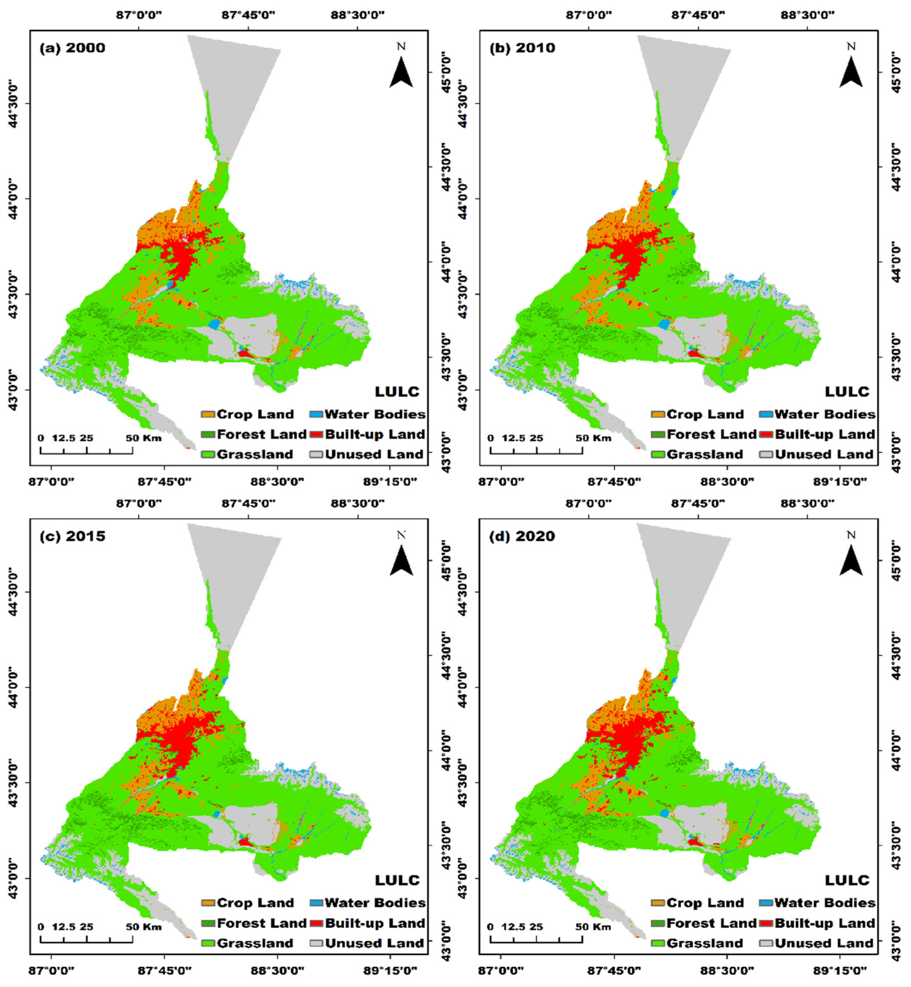
| Land Use Type | 2000 | 2010 | 2015 | 2020 | ||||
|---|---|---|---|---|---|---|---|---|
| Area (km2) | Percentage (%) | Area (km2) | Percentage (%) | Area (km2) | Percentage (%) | Area (km2) | Percentage (%) | |
| Cropland | 1221.01 | 8.60 | 1234.96 | 8.70 | 1157.49 | 8.13 | 1123.45 | 7.91 |
| Forest Land | 403.89 | 2.84 | 410.30 | 2.89 | 408.15 | 2.87 | 408.38 | 2.88 |
| Grassland | 7587.70 | 53.42 | 7541.62 | 53.10 | 7481.97 | 52.55 | 7413.27 | 52.20 |
| Water Bodies | 234.98 | 1.65 | 229.85 | 1.65 | 209.34 | 1.47 | 220.78 | 1.55 |
| Built-up Land | 584.66 | 4.12 | 626.45 | 4.41 | 822.15 | 5.77 | 884.59 | 6.23 |
| Unused Land | 4170.49 | 29.36 | 4159.55 | 29.29 | 4158.54 | 29.21 | 4152.26 | 29.24 |
| Variables | β | SE | t | SD | R2 | Adjusted R2 | AICc |
|---|---|---|---|---|---|---|---|
| NDVI | −4.90 *** | 0.16 | −30.20 | 0.14 | 0.58 | 0.58 | 887,149.50 |
| NDBI | 21.91 *** | 0.13 | 164.73 | 0.10 | |||
| UI | 7.65 *** | 0.08 | 90.48 | 0.08 | |||
| Slope | −0.11 *** | 0.01 | −60.71 | 0.01 | |||
| Intercept | 53.02 *** | 0.04 | 1065.32 | 0.03 |
| Diagnostics | Values |
|---|---|
| Residual sum of squares | 2,641,758.84 |
| AICc | 872,474.52 |
| R2 | 0.75 |
| Adjusted R2 | 0.73 |
| Bandwidth of GWR | 19,569.60 |
| Sigma | 6.02 |
Disclaimer/Publisher’s Note: The statements, opinions and data contained in all publications are solely those of the individual author(s) and contributor(s) and not of MDPI and/or the editor(s). MDPI and/or the editor(s) disclaim responsibility for any injury to people or property resulting from any ideas, methods, instructions or products referred to in the content. |
© 2023 by the authors. Licensee MDPI, Basel, Switzerland. This article is an open access article distributed under the terms and conditions of the Creative Commons Attribution (CC BY) license (https://creativecommons.org/licenses/by/4.0/).
Share and Cite
Ma, Y.; Mamitimin, Y.; Tiemuerbieke, B.; Yimaer, R.; Huang, M.; Chen, H.; Tao, T.; Guo, X. Spatiotemporal Characteristics and Influencing Factors of Urban Heat Island Based on Geographically Weighted Regression Model: A Case Study of Urumqi City. Land 2023, 12, 2012. https://doi.org/10.3390/land12112012
Ma Y, Mamitimin Y, Tiemuerbieke B, Yimaer R, Huang M, Chen H, Tao T, Guo X. Spatiotemporal Characteristics and Influencing Factors of Urban Heat Island Based on Geographically Weighted Regression Model: A Case Study of Urumqi City. Land. 2023; 12(11):2012. https://doi.org/10.3390/land12112012
Chicago/Turabian StyleMa, Yunfei, Yusuyunjiang Mamitimin, Bahejiayinaer Tiemuerbieke, Rebiya Yimaer, Meiling Huang, Han Chen, Tongtong Tao, and Xinyi Guo. 2023. "Spatiotemporal Characteristics and Influencing Factors of Urban Heat Island Based on Geographically Weighted Regression Model: A Case Study of Urumqi City" Land 12, no. 11: 2012. https://doi.org/10.3390/land12112012
APA StyleMa, Y., Mamitimin, Y., Tiemuerbieke, B., Yimaer, R., Huang, M., Chen, H., Tao, T., & Guo, X. (2023). Spatiotemporal Characteristics and Influencing Factors of Urban Heat Island Based on Geographically Weighted Regression Model: A Case Study of Urumqi City. Land, 12(11), 2012. https://doi.org/10.3390/land12112012