Article

Study on the Ecosystem Service Supply–Demand Relationship and Development Strategies in Mountains in Southwest China Based on Different Spatial Scales

1
Chinese Research Academy of Environmental Sciences, Beijing 100012, China
2
Lhasa Plateau Ecosystem Research Station, Key Laboratory of Ecosystem Network Observation and Modeling, Institute of Geographic Sciences and Natural Resources Research, Chinese Academy of Sciences, Beijing 100101, China
3
University of Chinese Academy of Sciences, Beijing 100049, China
*
Author to whom correspondence should be addressed.
Land 2023, 12(11), 2007; https://doi.org/10.3390/land12112007
Submission received: 1 October 2023 / Revised: 20 October 2023 / Accepted: 27 October 2023 / Published: 2 November 2023

Abstract

:
Mountainous regions typically exhibit a strained relationship between humans and the land, with noticeable spatial differences in the supply and demand of ecosystem services (ESS and ESD, respectively). ESS and ESD display varying characteristics at different spatial scales. Research on ESS and ESD at multiple scales can aid regional development and efficient ecosystem management. However, the current research focuses on ESS and neglects the ES characteristic changes at different scales. This study concentrates on the Hengduan Mountain region in southwest China. It evaluated ESS and ESD, analyzed the spatial matching relationship, and proposed a corresponding development strategy. The results demonstrated four key findings. First, ESS displayed an inverse spatial distribution on the two scales and was lower in the north and higher in the south at the raster scale. Over the period 2000–2020, ESS exhibited a pattern of initial increase, followed by a decrease, albeit with varying spatial patterns. Changes in land use primarily drove these ESS changes. Second, ESD increased from northwest to southeast on both scales and showed a rising trend over time. Third, at the grid scale, the low supply and low demand (L-L) region is primarily situated in the northwestern part, and it is crucial to prevent grassland degradation and manage grazing intensity. The low supply and high demand (L-H) region is located in the southeast, where the protection of cultivated land, along with comprehensive control of rocky desertification and debris flow, should be prioritized. High supply and low demand (H-L) are found in the northern mountain area, where paying attention to soil erosion control is essential. For areas with high supply and high demand (H-H) types, efforts should be directed toward maintaining forest habitat integrity. Fourth, on the county scale, L-H types should focus on realizing the ecosystem service value and implementing ecological agriculture. H-L counties can appropriately develop economic activities. Simultaneously, ecological compensation should be conducted among counties.

1. Introduction

According to the ecosystem services (ES) cascade framework [1], ecological functions, derived from ecosystem structures and processes, form ecosystem services. These services, in conjunction with other forms of capital, ultimately contribute to human well-being [2,3]. ESs, as an intermediate link in this process, effectively bridge the natural and social ecosystems, biogeographic processes, and human well-being [4,5,6,7,8]. Therefore, research on ESs requires a comprehensive study that involves multiple disciplines, including natural science, sociology, and management [4]. The supply and demand of ecosystem services (ESS and ESD, respectively) mirror the changes in natural and societal systems, respectively, which are crucial aspects of ecosystem service research [9,10]. At the natural ecosystem, climate change profoundly affects natural capital and ESS, leading to future uncertainty. At the same time, in socioeconomic systems, the rapid pace of urbanization and economic development will persistently escalate ESD. The discrepancy between the supply and demand of ecosystem services has given rise to a series of ecological issues [11]. For instance, to satisfy the demand for timber, extensive deforestation has occurred, leading to soil erosion and other ecological problems [12]. Based on the spatial difference analysis of ESS and ESD, the enrichment and shortage regions can be effectively identified, and different development strategies can be proposed for each region [13,14]. Policies will promote the balanced development of ESS and ESD by adjusting the land use intensity and other human activities, which will further help achieve the regional sustainable development goal [9].
Research on ESs has been conducted for many years, focusing primarily on ESS [15]. Numerous scholars have extensively studied the value of ESS [16,17], the quantitative assessment of individual ES [18,19], the trade-off among multiple ESs [20,21,22], and ecosystem service clusters [23,24]. These studies have significantly enriched the ES literature. The study of ESS is intrinsically linked to the study of ESD [25]. Currently, the research on ESS, ESD, and their corresponding relationships is in its nascent stage [26,27,28]. Various methodologies have been developed to examine the supply and demand of ecosystem services. The matrix method, proposed by Burkhard et al. [29], uses expert scores for various land use types as their ESS and ESD values, encompassing 22 ESs and 24 land use types. This method has seen enhancements and applications at the regional level [30,31,32] because it requires less data. However, it is intrinsically influenced by the quality of the experts and tends to exhibit subjectivity. Other researchers are focusing on individual ESs, evaluating ESS using ecological models, and considering ecosystem service usage as ESD. The methodologies differ across various ESs [5,9,33]. For instance, Sun et al. [34] employed this method to assess the supply and demand of a range of ESs, including soil and water conservation, carbon sequestration, and wood production in northeast China. While this method provides a detailed description of the supply and demand relationship for individual ES, the calculation process is complex. Compared with the first two methods, the third method considers the ecosystem services value (ESV), calculated using the equivalent method, as supply. It quantifies ESD based on economic and population data, thereby simplifying the assessment process to some degree and enriching the influencing factors. This method has been used in ecological protection and restoration zoning, as well as regional development strategies in numerous areas [13,14,35].
China is a country characterized by a broad distribution of mountains, with such terrain constituting approximately 70% of its total land area [36]. In the strategic planning for key ecosystem protection and restoration projects in China for the period 2021–2035, many mountainous regions, including Changbai Mountain, Nanling Mountain, Qinling Mountain, and Qilian Mountain, are incorporated within ecological barrier areas and ecological belts. This inclusion underscores the significant and diverse ecosystem service supply capabilities of these mountainous areas [37]. The direct use of land in mountainous regions is considerably limited, owing to substantial terrain variations, often resulting in a strained relationship between humans and the land [38]. Populations and urban areas are predominantly concentrated and distributed in relatively slow areas, and the level of ESS usually presents obvious vertical heterogeneity. Consequently, there are significant spatial differences in ESS and ESD within mountainous regions [39]. Mountainous regions are typically economically underdeveloped areas with minimal economic activity. In the context of urbanization and industrial advancement, these regions are also likely to experience rapid development, which will inevitably affect ESS and ESD. Conducting research on ESS and ESD in mountainous areas could support regional management strategies, facilitating a balance between regional ecology and economy. Moreover, ecogeographic elements, as well as ESS and ESD, display varying characteristics at different scales. The pronounced spatial heterogeneity resulting from the rugged terrain in mountainous regions further amplifies the differences in ESS and ESD across various scales. Studying ESS and ESD at different scales will assist in proposing effective management measures.
As an important ecological security barrier in China, southwest China has been listed as an important research area to conduct relevant ecosystem services research based on biophysical model assessment. However, existing studies mostly focus on the spatial characteristics of ecosystem service supply and its tradeoff effects [40,41,42], and there is a lack of ESD research in ecologically complex regions to a certain extent. In addition, it is not sufficient to explore the changes in ES characteristics in large spatial areas at different scales. In this study, we chose the Hengduan Mountain region (HD region), a location characterized by a complex relationship between humans and the land, as our research area. We evaluated the supply and demand of ESs over the past two decades and conducted matching analyses, focusing on changes at both grid and county levels. The objectives include (1) elucidating the drivers of ESS and ESD changes based on their spatiotemporal characteristics and (2) proposing different regional development strategies based on the corresponding analysis of ESS and ESD matching at different scales. The findings from this research are anticipated to offer scientific backing for regional development and ecosystem management.

2. Materials and Methodology

2.1. Study Area

The HD region, located in southwest China (Figure 1), exhibits a terrain that progressively increases from southeast to northwest. This region is primarily characterized by mountains and ravines. It boasts a variety of climate types and a rich vertical gradient of vegetation, leading to abundant biodiversity, particularly in northwest Yunnan. The HD region, being the upper reaches of numerous rivers and having a wide distribution of ecological land, provides significant ESs. However, the population distribution in the region is relatively concentrated, resulting in an uneven demand for these services. Consequently, there is a spatial mismatch between the distribution of ESS and ESD. This region, therefore, serves as an excellent example for studying the spatiotemporal variation of ESS and ESD.

2.2. Data source and Preparation

This study primarily uses land use data, derived from the 30 m land use interpretation data of Wuhan University, encompassing the years 2000, 2010, and 2020. Additionally, these data are employed to compute the comprehensive index of land use degree. The original data comprise nine categories: cropland, forest, shrub, grassland, water, snow/ice, barren land, impervious land, and wetland. Following the methodology of previous research [43,44], we consolidated shrubs with forest into a single category, and merged snow/ice into wetland, resulting in a seven-category land use data set. Data pertaining to grain production, sown area, and grain prices were sourced from the Statistical Yearbook. Spatial distribution data for population and gross domestic product (GDP) were obtained from the Resource and Environmental Science Data Center of the Chinese Academy of Sciences”https://www.resdc.cn/ (accessed on 1 September 2023)”.

2.3. Methods

2.3.1. Mapping ESS

In this study, we use ESVs as an index of ESS level. We refer to the framework of equivalent factors developed by Xie et al. [45], which provides an ESV assessment method specifically designed for China and has been employed extensively in ecosystem services research across various regions [13,35]. This method uses the natural grain production capacity (the grain yield of one hectare) of cultivated land as a benchmark to calculate the value of diverse ESs for other types of land use by multiplying the coefficient. We have calibrated the equivalent factor table with the assistance of vegetation growth data to make it suitable for the HD region [44].
We calculated the per unit area value of grain production for the years 2000, 2010, and 2020 for grain crops, which include soybeans, wheat, corn, and rice. Considering the influence of economic prices, we have converted the 2010 and 2020 values to constant 2000 prices [44]. Our results reveal that the per unit area grain production capacity of cultivated land in the HD region is 1000 CNY/ha. We posit that built-up land negatively affects the supply of ecosystem services. By consulting the relevant literature [46] and incorporating information from the HD region, we determined that the per unit area value of ESs for built-up land is −10,531.78 CNY/ha. ESS in the Hengduan Mountain area is calculated using the following formula:
E S S = i = 1 7 E i j × A j .
In this expression, Eij refers to the unit value of ESVi in ecosystem j, and Aj is the area of land type j.

2.3.2. Mapping ESD

Currently, scholars offer varying definitions of ESD. In this study, we concur with Villamagna et al. [47], who argue that ESD refers to the ecosystem services that humans can acquire or consume. The level of demand for ecosystem services is intimately tied to the level of socioeconomic development.
It is widely accepted that ESD is influenced by the extent of land use development, population density, and the level of economic development [13]:
E S D i = L U D i × lg ( P i ) × lg ( G i ) ,
where ESDi represents the ESD value of grid i, LUDi represents the degree of land use development in grid i, Pi represents the population in grid i, and Gi represents the GDP of grid i.
Drawing on the relevant literature [48], we allocated distinct values to various land use types to denote their respective degrees of development. Unused land was assigned a value of 1; forest, grassland, and water were assigned a value of 2; cultivated land was assigned a value of 3; and built-up land was assigned a value of 4. When a calculation unit contains multiple land use types, the degree of land use development is ascertained by the type of land use and its proportion. The higher the degree of land use development, the greater the need for ESD support. This yields the following formula:
L U D i = i = 1 n A i × S i S ,
where Ai is the grade of development intensity for the land use type, Si is the area of grade i land use, S is the total area of land use within the evaluation unit, and n is the graded number of land use degree.
The demand for ecosystem services increases with population growth. In this study, we use the GDP as an indicator of economic development. A higher GDP corresponds to a greater need for ecosystem services.

2.3.3. Matching the Degree of ESS and ESD

The four-quadrant method effectively illustrates the relationship between ESS and ESD and has been used in numerous studies [13,14]. The units of ESS and ESD can be removed through standardization, thereby facilitating a more effective comparison between the two. The following Z-score method is typically employed for standardization:
E S I = E S I i E S I ¯ s t d ( E S I ) ,
where ESI denotes the ES index (ESS or ESD), i stands for grid i,  E S I ¯ stands for the average value of ESI, and Std (ESI) is the standard deviation of ESI.
The normalized ESS and ESD values are matched and positioned in a two-dimensional coordinate system, with ESS on the x-axis and ESD on the y-axis. The first quadrant signifies a high supply and high demand (H-H type), the second quadrant indicates a low supply and high demand (L-H type), the third quadrant denotes a low supply and low demand (L-L type), and the fourth quadrant represents a high supply and low demand (H-L type). The H-L and L-H types depict two kinds of supply and demand mismatches, with H-L being the more desirable state.

3. Results

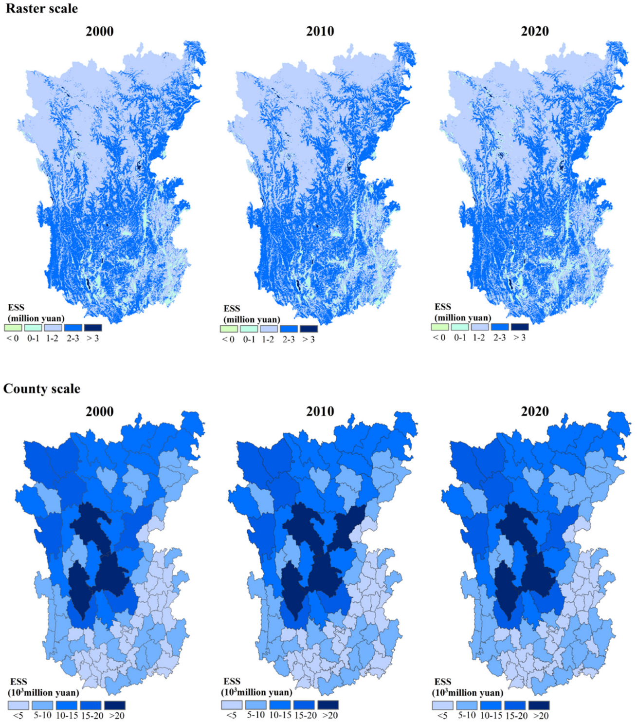
3.1. ESS at the Raster and County Scale

3.1.1. Spatial Distribution of ESS

On the raster scale, ESS exhibited significant spatial variations (Figure 2). We categorized ESS values, noting that areas with negative values are extremely limited, primarily coinciding with the regional county seat. The area where ESS ranged between CNY zero and one million was small, constituting only 4.28% of the entire region (using the year 2000 as a reference). These areas were dispersed in low-lying intermountain basins or valleys in the southern part of the study area, such as the Anning River Valley in Xichang, Xundian Basin in Xundian and Chongming counties, basins in Binchuan and Xiangyun counties, and Lijiang Basin. The regions where ESS ranges between CNY one and two million were predominantly located in the north and southeast of the study area, covering approximately 56.29% of the total area. Specifically, the northern part encompasses Jiangda–Gongjue counties, areas from Serta to Litang counties, and most of Aba and Hongyuan counties. The southeastern part included the southwest of Sichuan Basin (Xide, Meigu, and Zhaojue counties) and the southeast corner of the HD region (Qiaojia–Huize–Xundian counties). Regions with an ESS between CNY two and three million were widely dispersed (accounting for about 39.11% of the entire region) and primarily concentrated in the southern part of the HD region, areas surrounding river valleys in the northern part, and the northwestern edge of Sichuan Basin. The areas in the north extend along major rivers, such as the Lancang River, Jinsha River, Yalong River, and Dadu River, exhibiting a tree-branching distribution. The area with an ESS above CNY three million is a mere 0.31% and is scattered.
At the county scale, ESS exhibited a distribution pattern distinct from that observed at the raster scale. Overall, ESS values ranged from CNY 27 million to 27,722 million. Counties with ESS values less than CNY 5000 million were primarily located in the southeastern region, including Ganluo, Meigu, Zhaojue, Puge, Qiaojia, Miyi, and Yongren counties, as well as the southern part of the HD region, such as Jianchuan, Heqing, Binchuan, Xiangyun, and Yaoan counties. Counties with ESS values ranging from CNY 5000–10,000 million were primarily in the south, including Huidong and Lufeng counties in the southeast, and counties along the three parallel rivers in the west, extending from Gaongshan to Yongping counties. This group also includes some counties in the central region, such as Derong and Xiangcheng, along with some northeastern counties ranging from Heishui to Baoxing, Jinchuan, Danba, and Luhuo. Eighteen counties, primarily located in the northern region, including areas from Garze to Jiuzhaigou and Xinlong–Daofu–Yajiang, Xiaojin, as well as some western counties, such as Chayab, Deqin, and Batang, have an ESS value fluctuating between CNY 10,000 and 15,000 million, with a relatively concentrated distribution. Seven counties, including Jiangda, Dege, Baiyu, and Mangkang in the northwest, Kangding in the east, and Yanyuan and Lijiang Gucheng in the central region, have ESS values ranging from CNY 15,000 to 20,000 million. Only three counties, namely Litang, Muli, and Shangri-La, located centrally, have ESS values exceeding CNY 20,000 million.

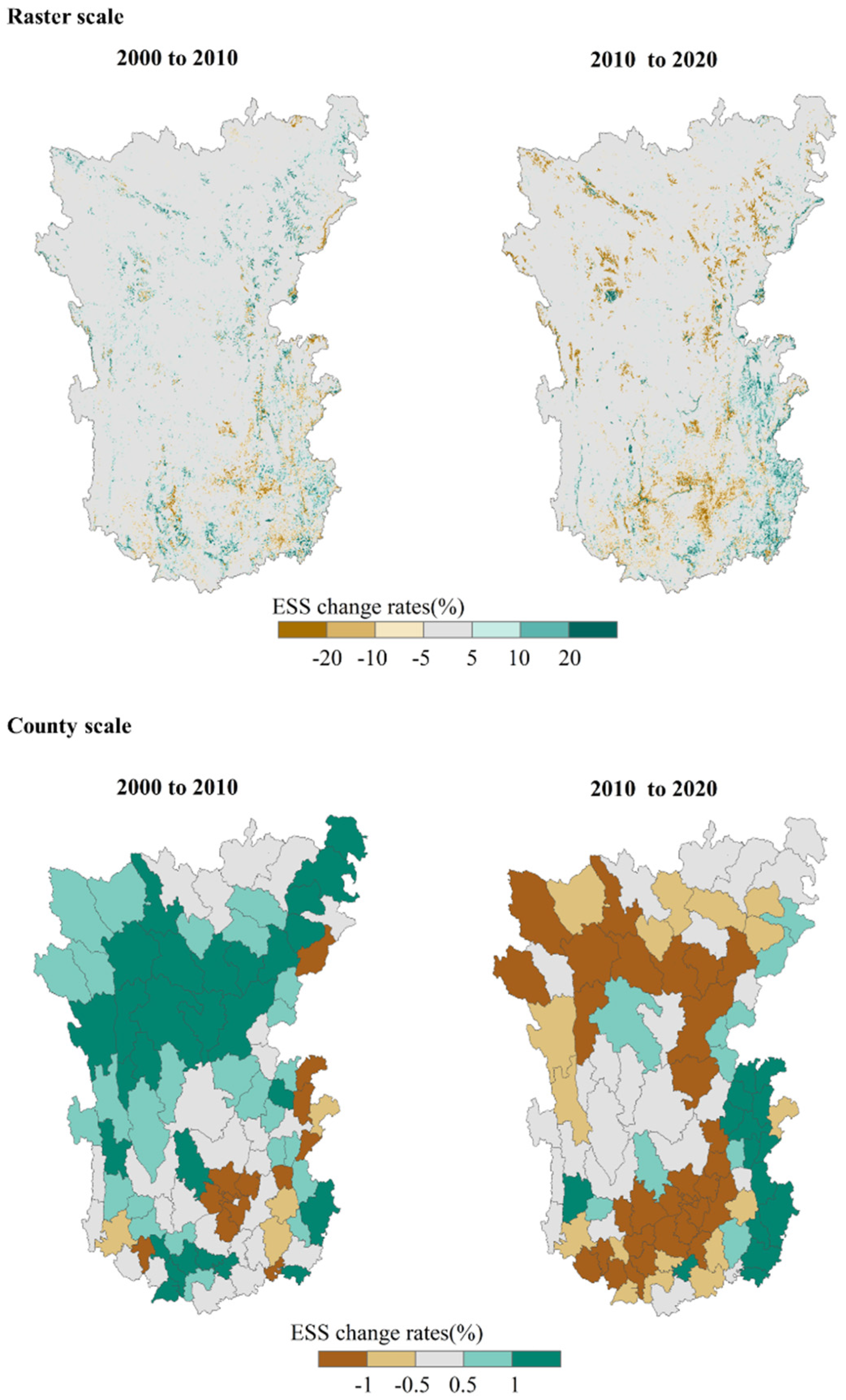
3.1.2. Temporal Changes of Ecosystem Service Supply

In terms of total value, the ESS of the HD region was valued at CNY 787 billion in 2000 and CNY 792 billion in 2010. We assessed the rate of ESS changes from 2000 to 2010 and 2010 to 2020 on a raster scale, considering changes between −5% and 5% as stable. Overall, areas with stable ESS values accounted for approximately 83.34–85.96% of the total from 2000 to 2020 (Figure 3).
In the HD region, areas with declining ESS values represented approximately 5.52% from 2000 to 2010, while areas with increasing ESS values were more extensive, constituting about 8.52% of the entire region. In the southern part of the HD region, the areas of ESS increase and decrease were interspersed. Most areas with ESS increases were situated in mountainous regions, such as the high-altitude areas in the southeast corner of the HD region, the mountainous areas stretching from Heqing to Dali and Xiangyun county in the southwest, the mountainous areas of Yongping in the southwest corner, and the valley extending from Weixi to Lanping. The regions exhibiting a decrease in ESS are primarily flat areas, including the vicinity of Panzhihua, the mountain valley bordering Heqing and Yongsheng counties, and the valley and basin stretching from Xichang to Yanyuan and Dechang. Conversely, in the northern section, ESS predominantly displayed an increasing trend, notably in the mountainous region in the northeast, the mountainous terrain from Dege to Luhuo, and the areas extending from Mangkang to Kangding.
Between 2010 and 2020, the total ESS values in the HD region exhibited a decreasing trend, with the value in 2020 amounting to CNY 788 billion. Approximately 9.68% of the areas showed a decrease in ESS values, while about 6.98% demonstrated an increase (Figure 3). Spatially, the southern part of the region displayed a staggered pattern of ESS increases and decreases. The regions with increased ESS values were primarily located in mountainous areas, such as those stretching from Ganluo to Xundian county on the eastern side of the HD region, and the Lanping county section of the Lancang River valley. Conversely, areas with decreased ESS values were found in relatively flat regions, such as the basin in Panzhihua–Yongren–Yuanmou–Huili, the Anning River valley in Xichang, and the basin in Heqing–Binchuan–Yongsheng counties. The ESS value primarily decreased in the northern region, particularly in higher elevations, like the mountainous areas from Dege to Luhuo counties, and the mountainous areas of Jiangda county. The regions with increased ESS values were limited, including the Dadu River and Minjiang River valleys.
At the county scale, we classified change rates between −0.5% and 0.5% as stable (Figure 3). The proportions of stable areas from 2000 to 2020 were approximately 27.27% and 32.72%. From 2000 to 2010, the primary changes in ESS were increases, with 53 counties accounting for about 63.55% of the HD region. These counties were predominantly located in the northern part, as well as the southeastern and southwestern edges. ESS values showed a decreasing trend in 12 counties, which accounted for about 9.18% of the total area. These counties were primarily situated around Panzhihua and the areas from Ebian to Jinyang county. From 2010 to 2020, the numbers of counties with ESS increases and decreases were 23 and 48, respectively, representing approximately 18.65% and 48.63%, respectively, of the entire HD region. Counties with increased ESS included the eastern part (from Maoxian to Chongming) and some western counties. Counties with reduced ESS were mainly located in the northern and southern regions.

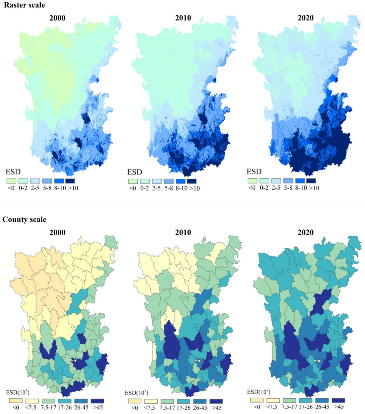
3.2. ESD for Raster and County Scale

3.2.1. Spatial Patterns for ESD at Different Scales

ESD exhibited significant spatial variations on the raster scale. Overall, it demonstrated an upward trend from the northwest to the southeast (Figure 4). Areas with low values were continuously distributed, while those with high values were dispersed. For instance, in 2000, regions with ESD values below zero were located primarily in the northwest, encompassing most of Ganzi Prefecture and the northern part of Qamdo. Regions with ESD values between 0 and 2 were adjacent to those with ESD values below zero, including Aba Prefecture, eastern Ganzi, southern Qamdo, northwestern Liangshan Prefecture, and Diqing Prefecture. Areas with ESD values between 2 and 5 were situated primarily around Sichuan Basin, southwestern Liangshan Prefecture, Lijiang, and the western part of Dali Prefecture. ESD values between 5 and 10 were continuously distributed in the southeastern and southern regions of the HD region. The distribution of areas with ESD values exceeding 10 was relatively scattered, including Xichang, Huize County, Panzhihua, Dali, and so on.
The distribution of ESD at the county level differs from the raster level. Overall, ESD was lower in the northwestern counties and higher in the southeastern region. For instance, in 2000, the northwestern area of the study region (encompassing Jiangda, Dege, Chaya, Gongjue, Baiyu, Xinlong, Yajiang, Litang, Batang, Daocheng counties, and so on) exhibited negative ESD values, affecting a total of 11 counties. Approximately 22 counties had ESD values ranging from 0 to 7500, located primarily in the northeastern, central, and west–central regions of the HD region. Specifically, these counties included most of the counties in Aba Prefecture, Luhuo, Ganzi, Daofu, Danba, Jiulong, Xiangcheng, Derong, and Luding counties in Ganzi Prefecture, Muli county in the central part, and Deqin, Gongshan, Mangkang, and Fugong counties in the western part. Counties with ESD values ranging from 7500 to 17,000 were located primarily along the eastern line of the HD region (from Maoxian to Tianquan counties), in the southwest portion of Sichuan Basin (west of the Shimian–Ganluo–Ebian–Yuexi–Xide–Puge–Dechang–Miyi counties and north of Ningnan), in the southwest part (areas of Shangri-La–Ninglang–Yanbian–Huaping–Yuanmou–Chongming counties), and the southwest edge region. Counties with ESD values ranging from 17,000 to 26,000 were more concentrated, including the areas of Qiaojia–Huidong–Luquan–Xundian in the southeast, Yongsheng-Dayao–Binchuan–Xiangyun–Eyuan counties in the southwest, and Yanyuan, Mianning, and Kangding in the north. Only seven counties, namely Huili, Xichang, Panzhihua, Huize, Lufeng, Chuxiong, and Lijiang, had ESD values exceeding 26,000.

3.2.2. ESD Evolution from 2000 to 2020

On a raster scale, the mean ESD in the HD region was 2.46, 4.23, and 5.72 for the years 2000, 2010, and 2020, respectively, indicating an upward trend. Spatially, almost all regions exhibited an increase in ESD values (Figure 4); thus, we did not employ change rates to depict temporal variations. From 2000 to 2010, the area with an ESD less than zero significantly decreased, from 26.25% to 0.09%, primarily in the northwestern part of the HD region. The area with an ESD value between 2 and 5 rose from 17.80% in 2000 to 19.43% in 2010, with the increase predominantly located in the northeastern part (from Heishui to Xiaojin and Jiulong counties), Jiuzhaigou county, and Shangri-La. The areas that decreased were mainly located in the southwest of Sichuan Basin (Ebian–Meigu–Butuo counties), Yanyuan county, and the areas of the Yongsheng–Yongren–Lijiang–Yangbi–Yongping–Lanping counties, and the ESD value in these areas increased, fluctuating between 5 and 8. For the areas where the ESD value ranged from 5 to 8 in 2000, the ESD value rose to more than 8. Notably, in Xiangyun, Dali, Panzhihua, Xichang, Huize, Dongchuan, Chongming, and Fumin, the increase was substantial, with the value in 2010 exceeding 10. The regions with an ESD between 8 and 10, as well as those higher than 10, expanded. The areas increased from 3.70% and 2.46% to 8.58% and 10.23%, respectively. From 2010 to 2020, the proportion of the region with ESD values between 0 and 2 diminished (to 21.89% in 2020). This reduction primarily occurred because the ESD value in some regions rose to the 2–5 range. These areas encompass most of the counties, excluding Litang county. Consequently, the regions with an ESD between 2 and 5 expanded (to 35.88% in 2020). For the majority of areas with an ESD between 5 and 8 in 2010, the value increased and fluctuated between 8 and 10. For areas with an ESD between 8 and 10 in 2010, the value increased to more than 10.
At the county level, ESD values exhibited a spatially increasing trend between 2000 and 2020 (Figure 4). From 2000 to 2010, the spatial range of counties with ESD values less than zero diminished, with ESD values rising to the 0–7500 and 7500–17,000 ranges. In most counties where the ESD value was between 0 and 7500, ESD values escalated to the 7500–17,000 range, with Jiulong and Muli experiencing a more significant increase to the 17,000–26,000 grade. For counties with ESD values between 7500 and 17,000, approximately 53.65% saw an increase in ESD by one grade. Ninglang and Lanping counties witnessed a two-grade increase (26,000–45,000 in 2010), while Shangri-La experienced the most substantial increase, reaching the highest grade. Most counties with an ESD value in the range of 17,000–26,000 experienced an increase of one grade, with Yanyuan county showing a more significant increase (exceeding 45,000 in 2010). Among the counties in the 26,000–45,000 grade, four experienced an increase. From 2010 to 2020, among the counties with an ESD value less than 7500, 11 counties showed an increase of one degree, while the rest increased by two degrees. For the counties in grade 2 (7500–17,000), over 60% experienced an increase of one grade in their ESD value. In grade 3 (17,000–26,000), the counties with increased ESD values were primarily located in Yanbian–Miyi–Dechang and the southwestern part of the HD region. For counties with an ESD value between 26,000 and 45,000, only Kangding, Yongsheng, and Xichang experienced an increase in their ESD grade.

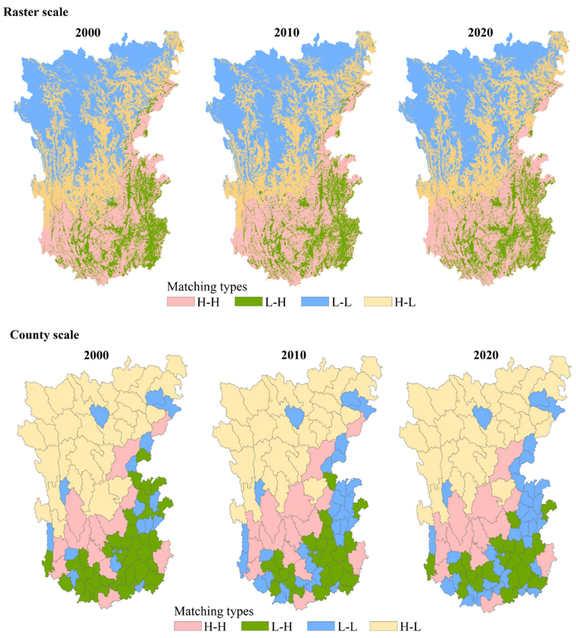
3.3. Matching ESS and ESD

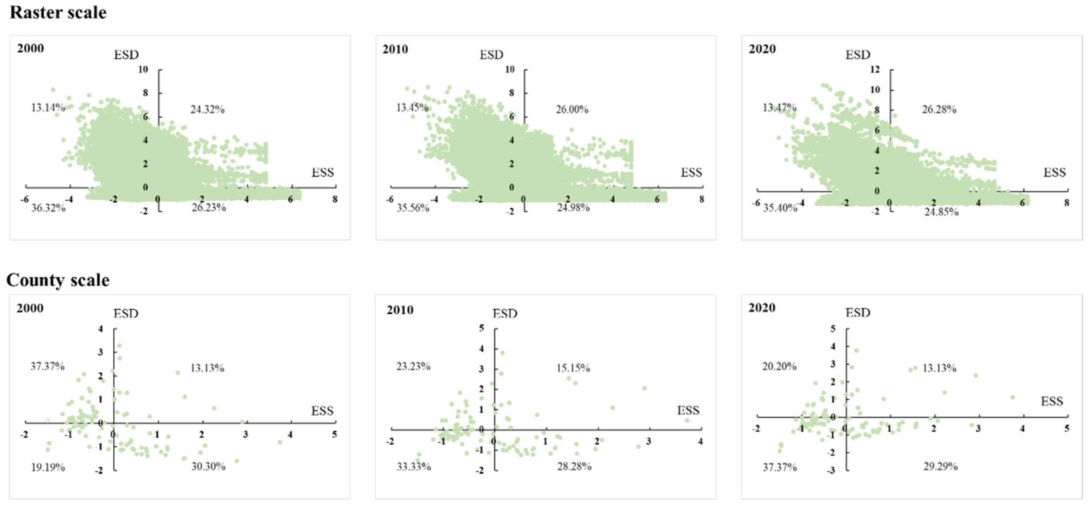
3.3.1. Four-Quadrant Analysis and Spatial Distribution of Matching Types

The dot plots for 2000, 2010, and 2020, when mapped onto a two-dimensional coordinate system of ESS and ESD, are similar (Figure 5). Approximately 24.32% of the entire region demonstrated a high supply and high demand (H-H) type, predominantly located in the first quadrant. These areas, characterized by a higher ESV than ESD, were primarily situated in the southern part of the Hengduan Mountain (HD) region and were continuously distributed. Specifically, they encompassed the southwestern part of the HD region, the edge of Sichuan Basin in the eastern edge, the central southern region, and the southern edge (Figure 6). The areas classified as low supply and high demand (L-H) type, located in the second quadrant, constituted about 13.14% of the HD region, with a relatively uniform distribution of the two components. The areas primarily lay in the southern part of the line connecting Songpan, Xiaojin, Kangding, Jiulong, Muli, Ninglang, Shangri-la, and Weixi counties. These areas predominantly encompass large river valleys, such as the Anning valley stretching from Mianning to Panzhihua, the Jinsha River valley in the southeast, and the valley from Yongsheng county to Binchuan county. They also included intermountain basins (like Yuanmou Basin), and the eastern margin, which was the east side of the line connecting Ganluo, Yuexi, Xide, Ningnan, Huidong, Xundian, and Chongming counties. The matching relationship between ESS and ESD falls into the L-L category (third quadrant), approximately 36.32% of the HD region. In these areas, ESS exhibited minimal variation, while ESD fluctuated significantly. Geographically, the L-L types primarily appeared in contiguous patches in the northern part of the study area. The H-L type (fourth quadrant) accounts for about 26.23% of the total study area. In this category, ESD showed little variation, while ESS varied considerably. The H-L types are predominantly found in the north–central region, particularly around the river valleys, exhibiting a dendritic distribution pattern. Large areas were concentrated along the Weixi–Deqin–Shangri-La–Ninglang–Muli–Jiulong line, as well as in the Yajiang, Danba, Lixian, Heishui, and Jiuzhaigou counties in the northern part.
At the county level, approximately 13.13% of the counties demonstrated an H-H type, with ESS and ESD being evenly distributed. Spatially, this includes the northwest of Yunnan Province and the west of Liangshan Prefecture, primarily encompassing the Yunlong–Lijiang–Shangri-La–Ninglang–Yongsheng–Yanyuan–Mianning area, Kangding and Wenchuan counties in the north, and Huize county and Chuxiong City in the south. L-H counties were predominantly located in the southern part of the study area, making up 37.37% of the total counties. Specifically, these are in the southeast region, the southwest edge of Sichuan Basin, and the southwest region. The L-L type is dispersed, encompassing 19 counties. In terms of spatial distribution, it includes northern counties, such as Luhuo, Heishui, Maoxian, and others, as well as Meigu, Puge, Butuo, and Jinyang in the eastern part of Liangshan Prefecture. Collectively, these counties occupy a relatively small area. The H-L type includes 30 counties, situated primarily in the majority of the northern part of the HD region. More specifically, these counties were located west of the Jiuzhaigou–Songpan–Barkam–Xiaojin–Yajiang–Jiulong line and north of the Gongshan–Weixi–Xiangcheng–Daocheng–Muli line.

3.3.2. Time Evolution of Four Matching Types

At the grid scale, the most significant change from 2000 to 2020 was in the H-H and H-L types. The area proportion of the H-H type increased, rising from 24.32% to 26.00% and ultimately reaching 26.28%. Conversely, the area of the H-L type gradually decreased, falling from 26.23% to 24.98%, and ultimately reaching 24.85%. From 2000 to 2010, the regions primarily experiencing a transition from H-L types to H-H types were located in the central part of the study area, specifically, southern Weixi County, southern Shangri-La, southern Ninglang County, and the northeastern and western parts of Yanyuan County. Conversely, the areas where H-H types transitioned to H-L types were predominantly found in Baoxing county, situated in the northeastern part of the HD region. From 2010 to 2020, the areas where H-L types transitioned to H-H types were located primarily in Fugong county, parts of northern Ninglang, and parts of northern Weixi county. The regions where H-H types transitioned to H-L types were located in the central part of Shangri-La.
At the county level, the primary type of change was the conversion between L-H to L-L. The area of L-H steadily decreased, while L-L exhibited an increasing trend. From 2000 to 2010, counties transitioning from L-H to L-L were located primarily in the southwest of Sichuan Basin and some counties in Chuxiong and Dali Prefecture. From 2010 to 2020, counties that transitioned from L-H to L-L included Shimian in the central region, and Dechang, Songming, and Nanhua counties in the southern region.

4. Discussion

4.1. Multiple Factors Influencing ESS and ESD and Their Relationship

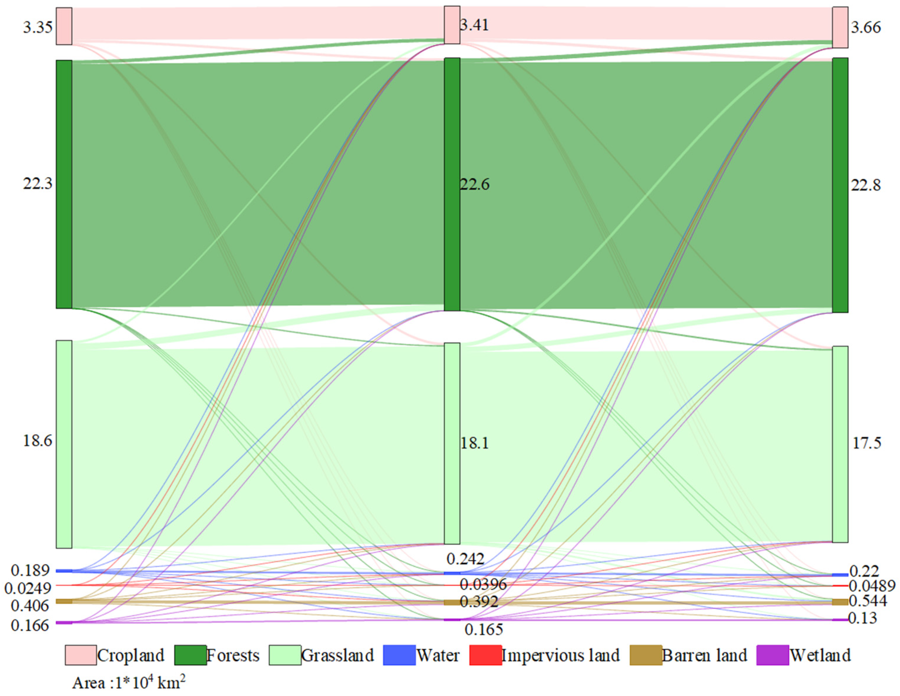
4.1.1. The Effects of Land Use Type and Its Change

Land use change, as the most direct and universal manifestation of human activities, influences the supply and demand capacity of ecosystem services to a certain degree [49,50,51,52]. In general, natural ecosystems, such as forests, grasslands, and water bodies, exhibit a more comprehensive eco-geographical process and a higher level of ESS compared to cultivated and built-up lands [38]. Owing to its complex structure, a forest has a higher ESS than a grassland. Consequently, at the grid scale, the ESS value was lower in the cultivated area of the valley in the southeast of the HD region and was higher in the forested area with higher elevation. At the county level, the ESS value is influenced not only by the type of land use but also by the county’s area. Consequently, it differs from the spatial distribution at the raster scale. For instance, while grassland and forest were the predominant land use types in Chaya and Yunlong counties, respectively, the ESS value in Chaya is higher, owing to its larger area. Overall, ESS values in the northwestern counties were generally higher, primarily because of their larger areas.
In terms of temporal change, ESS and land use change demonstrated significant spatial consistency. From 2000 to 2020, the most drastic changes occurred in cultivated land, forests, and grassland (Figure 7). Cultivated land and forests consistently increased, while grassland exhibited a decreasing trend (Figure 7). A prolonged period of overuse and devastation of the Yangtze River Basin has resulted in a range of ecological issues [12]. To alleviate some environmental problems such as local soil erosion, China implemented the “Forest Rehabilitation from Slope Agriculture” policy to promote afforestation in high slope cultivated lands around 2000 [53]. Simultaneously, the second phase of the “Protection Forest System Construction in the Yangtze River Basin” and the “Natural Forests Conservation Project” [54] were initiated. Consequently, cultivated lands and grasslands were transformed into forests, leading to a rapid expansion of the forest area at a growth rate of 1.35%.
Under the influence of cultivated land protection policies [55], suitable expansion of cultivated land was conducted in areas with gentle terrain, which was conducive to the development of agricultural mechanization and modernization to a certain extent. Additionally, some unused land was converted, owing to climate change. Changes in land use led to alterations in ESS at both the raster and the county scales. For instance, in the relatively flat region of Panzhihua, the transformation of forest into cultivated land led to a decrease in ESS. Conversely, in the mountainous area of Yongping county, the conversion of cultivated land into forest resulted in an increase in ESS. The rise in ESS in the mountainous region of Qiaojia county in the southeast and the northeast part of the HD region was primarily due to the conversion of grassland into forests. Furthermore, some ecosystem services increased in the northern part, which was linked to the transformation of unused land into grassland or wetlands.
Following 2010, China executed comprehensive land consolidation, transforming grassland, the primary reserve resource, into cultivated land. From 2010 to 2020, the expansion of cultivated land accelerated, growing at roughly four times the rate of the previous period. Concurrently, forest land area also increased as a result of earlier ecological projects. Overall, ESS in the HD region exhibited a decline during this period. ESS increase in the southeastern region resulted primarily from the conversion of grassland and cultivated land into forest in mountainous areas. ESS reduction in the southern Anning valley and other basins was largely because of the conversion of grassland into cultivated land. ESS decrease in the northern region was linked to the degradation of grasslands and wetlands, as wetlands decreased and unused land increased.

4.1.2. Driving Role of Economic Development

At both the raster and county scales, ESD in the northwest portion of the HD region was lower than in the southeast, a distribution that aligns spatially with the “Hu line”. The northwest side of the Hu line, characterized by sparse population, limited cultivated and built-up land, and less active economic activities, has a lower demand for ecosystem services.
The data reveal a clear upward trend in ESD values at both raster and county scales from 2000 to 2020, reflecting the continuous advancement of regional urbanization over the past two decades. In 2000, 2010, and 2020, the built-up land areas were 249 km2, 396 km2, and 489 km2, respectively, indicating an increased demand for ecosystem services. Since 2000, China has implemented the “Development of the Western Region” policy [56], significantly boosting the economy of southwest China. However, areas such as Liangshan Prefecture, Nujiang Prefecture, and Tibetan areas in the HD region were deeply impoverished areas in China [57,58,59], with some counties experiencing extreme poverty [60,61]. From 2010 to 2020, the Chinese government implemented a poverty alleviation policy, targeting poverty in all regions and eliminating county-level poverty by 2020. In 2017, the “Rural Revitalization Strategy” was introduced, invigorating the development of mountainous areas. This rapid economic development has increased the demand for ecosystem services.

4.2. Management Measures for the Spatial Pattern of Ecological Restoration

The supply and demand of ecosystem services embody both natural and societal attributes. These are influenced by the ecological environment and social organizations, including varying stakeholder needs [62]. In theory, according to the mechanism of “structure-process-ES”, changes in land use composition and configuration profoundly affect the relationship between ESS and ESD [63,64]. For example, the study of Hangzhou shows that the effects of land composition and configuration on the ESS-ESD matching relationship are 0.234 and 0.082, respectively [65]. Therefore, the corresponding relationship between ESS and ESD can be used as the main method of achieving regional landscape planning and fine ecosystem management in practice. In addition, the relationship between the supply and demand of these services exhibits scale differences. For instance, the matching relationships between ESS and ESD in the HD region displayed distinct spatial patterns at both the raster and county scales. Consequently, it is necessary to propose different development strategies for different spatial scales to effectively implement integrated management.
On a county scale, the L-H type, which includes counties in the Anning River Valley region and some southwestern counties, is the least ideal match. These areas have a significant distribution of cultivated land, a concentrated population, and a relatively developed economy. While nature determines the basic level of ecosystem service provision, human efforts can enhance it. These counties should prioritize improving the supply capacity of ecosystem services and hastening the realization of ecological product value. The development of ecological agriculture can enhance the ESS level of cultivated land in an environmentally friendly way. H-L counties were primarily in the study area’s northwest, where ESS can satisfy human needs. Some economic activities could be suitably conducted in this region. Moreover, ecosystem service flows exist in large-scale regions, and regions with high ESS provide substantial support for other regions with low ESS, even at the cost of their own economic development. Therefore, an ecological compensation policy should be implemented among counties. In particular, L-H counties should economically compensate H-L counties.
The L-H region, primarily located in the southeast of the study area, contains a large amount of cultivated land. However, this region also experiences some rocky desertification and is prone to debris flows, making its ecology relatively fragile. This fragility has become a limiting factor in enhancing ESS. Cultivated land is crucial for the food security of the regional population. In recent years, the Chinese government has implemented several policies to protect this land. For this region, it is necessary to protect the area and quality of cultivated land effectively, establish permanent basic farmland, and strictly regulate urban development boundaries to minimize encroachment on cultivated land. Additionally, measures should be taken to control and prevent rocky desertification and debris flows. The L-L type area, mainly located in the northwest of the study area, is a high-cold region with grassland as the predominant vegetation type. This region is susceptible to climate change and other factors. With sparse population distribution and a relatively underdeveloped economy, protecting the grassland from degradation and avoiding overgrazing are essential strategies to improve the ecosystem service supply level in this region.
The H-L type area, situated in the northern mountainous regions of the study area, is characterized by extensive forests and minimal human activity, owing to the challenging terrain. This region faces ecological issues, such as soil erosion. Ecosystem management should focus on preserving forest cover and combining biological and engineering measures to mitigate soil loss. Conversely, the H-H region, primarily located in the south, including northwest Yunnan, boasts abundant forest resources and relative economic prosperity. This region is a biodiversity hotspot, and biodiversity plays a crucial role in maintaining the balance of ecosystem service supply and demand. Therefore, ecosystem management in this region should prioritize maintaining habitat integrity and forest ecosystem connectivity.

4.3. Limitations and Prospects

First, this study assesses the supply and demand of regional ecosystem services using the value equivalent method and economic data. However, it does not discuss individual ecosystem services, such as soil conservation, carbon sequestration and oxygen release, and habitat quality maintenance. There are significant differences in the supply and demand assessments of various ecosystem services. Future work should select evaluation methods for different types of services and conduct evaluations and quantifications at various spatial scales. Second, the study uses a 1 km resolution grid scale and county scale at the administrative level. However, the supply and demand of ecosystem services vary on other resolution grids and administrative units, necessitating further scale research. Third, we analyze three periods: 2000, 2010, and 2020. Future work should consider multiple time scales to further analyze changes in ESS and ESD over different periods and their responses to land use change, economic development, and policy changes.

5. Conclusions

We conducted ESS and ESD research in a mountain area using the framework of the “ESS evaluation-ESD evaluation-matching relationship analysis”. Our conclusions are as follows.
First, at both the raster and county scales, ESS displayed contrasting spatial patterns. On the raster scale, ESS values were lower in the northern region, while ESS values were higher in the southern region. The size of the county area influenced ESS at the county scale, with higher values in the northwest and lower values in the southeast.
Second, in terms of temporal changes, the conversion of cultivated land, forests, and grassland, as well as the conversion of unused land, primarily drove ESS changes. From 2000 to 2010, the area where ESS increased was larger than where it decreased. However, from 2010 to 2020, the area where ESS decreased was larger than where it increased.
Third, ESD values rise from the northwest to southeast at both the raster and county scales. The southeast corner of the study area emerges as an area with very high ESD values, owing to the higher local economic level and land development intensity. Over time, in most regions, ESD values displayed an increasing trend from 2000 to 2020.
Fourth, at the raster scale, ESS and ESD primarily exhibited an L-L type. This area should focus on grassland protection, the prevention of grassland degradation, and the control of grazing intensity. The L-H type was situated primarily in the southeast, where comprehensive control of rocky desertification and debris flow should be considered while protecting cultivated land. For the H-L type area, soil erosion control should be a priority. In terms of the H-H type, maintaining the integrity of forest habitats should be emphasized.
Fifth, the matching relationship at the county level differs from the raster level. In counties with an L-H type, farmland is more prevalent. Future development should focus on enhancing and realizing the value of ecosystem services, which is achievable through the integration of agriculture and other industries. In H-L counties, economic activities can be suitably developed. At the same time, ecological compensation should be promoted at the county level, particularly where L-H counties provide economic compensation to H-L counties.

Author Contributions

Conceptualization, E.D.; Methodology, Y.W.; Software, Y.W. and Y.F.; Investigation, Y.W.; Resources, Y.Q.; Writing—original draft, Y.W.; Writing—review & editing, E.D.; Supervision, E.D. All authors have read and agreed to the published version of the manuscript.

Funding

This work was supported by the National Natural Science Foundation of China (42001262, 41571098) and the China Postdoctoral Science Foundation (2020M670436).

Data Availability Statement

Data sharing is not applicable to this article.

Conflicts of Interest

The authors declare no conflict of interest.

References

  1. Haines-Young, R.; Potschin, M. The Links between Biodiversity, Ecosystem Service and Human Well-Being. In Ecosystem Ecology: A New Synthesis; Raffaelli, D., Frid, C., Eds.; Cambridge University Press: Cambridge, UK, 2010; pp. 235–268. [Google Scholar]
  2. Costanza, R.; de Groot, R.; Sutton, P.; van der Ploeg, S.; Anderson, S.-J.; Kubiszewski, I.; Farber, S.; Turner, R.-K. Changes in the global value of ecosystem services. Glob. Environ. Chang. 2014, 26, 152–158. [Google Scholar] [CrossRef]
  3. Costanza, R.; de Groot, R.; Braat, L.; Kubiszewski, I.; Fioramonti, L.; Sutton, P.; Farber, S.; Grasso, M. Twenty years of ecosystem services: How far have we come and how far do we still need to go? Ecosyst. Serv. 2017, 28, 1–16. [Google Scholar] [CrossRef]
  4. Zhang, C.; Li, J.; Zhou, Z.; Liu, X. Research progress on the cascade effect of ecosystem service. Chin. J. Appl. Ecol. 2021, 32, 1633–1642. [Google Scholar]
  5. Wang, L.; Zheng, H.; Wen, Z.; Liu, L.; Robinson, B.E.; Li, R.; Li, C.; Kong, L. Ecosystem service synergies/trade-offs informing the supply-demand match of ecosystem services: Framework and application. Ecosyst. Serv. 2019, 37, 100939. [Google Scholar] [CrossRef]
  6. Mcdonald, R. Ecosystem service demand and supply along the urban-to-rural gradient. J. Conserv. Plan. 2009, 5, 1–14. [Google Scholar]
  7. Geijzendorffer, I.R.; Martín-López, B.; Roche, P.K. Improving the identification of mismatches in ecosystem services assessments. Ecol. Indic. 2015, 52, 320–331. [Google Scholar] [CrossRef]
  8. Mouchet, M.A.; Lamarque, P.; Martín-López, B.; Crouzat, E.; Gos, P.; Byczek, C.; Lavorel, S. An interdisciplinary methodological guide for quantifying associations between ecosystem services. Glob. Environ. Chang. 2014, 28, 298–308. [Google Scholar] [CrossRef]
  9. Shen, J.; Li, S.; Wang, H.; Wu, S.; Liang, Z.; Zhang, Y.; Wei, F.; Li, S.; Ma, L.; Wang, Y.; et al. Understanding the spatial relationships and drivers of ecosystem service supply-demand mismatches towards spatially-targeted management of social-ecological system. J. Clean Prod. 2023, 406, 136882. [Google Scholar] [CrossRef]
  10. Chaplin-Kramer, R.; Sharp, R.P.; Weil, C.; Bennett, E.M.; Pascual, U.; Arkema, K.K.; Brauman, K.A.; Bryant, B.P.; Guerry, A.D.; Haddad, N.M.; et al. Global modeling of nature’s contributions to people. Science 2019, 366, 255–258. [Google Scholar] [CrossRef] [PubMed]
  11. Millennium Ecosystem Assessment (MA). Ecosystems and Human Well-being: Synthesis; Island Press: Washington, DC, USA, 2005; Volume 5, p. 563. [Google Scholar]
  12. Xu, W.; Xiao, Y.; Zhang, J.; Yang, W.; Zhang, L.; Hull, V.; Wang, Z.; Zheng, H.; Liu, J.; Polasky, S. Strengthening protected areas for biodiversity and ecosystem services in China. Proc. Natl. Acad. Sci. USA 2017, 114, 1601–1606. [Google Scholar] [CrossRef]
  13. Peng, J.; Yang, Y.; Xie, P.; Liu, Y. Zoning for the construction of green space ecological networks in Guangdong Province based on the supply and demand of ecosystem service. Acta Ecol. Sin. 2017, 37, 4562–4572. [Google Scholar]
  14. Xie, Y.; Zhang, S.; Lin, B.; Zhao, Y.; Hu, B. Spatial zoning for land ecological consolidation in Guangxi based on the ecosystem services supply and demand. J. Nat. Resour. 2020, 35, 217–229. [Google Scholar]
  15. Wang, L.; Zheng, H.; Chen, Y.; Ouyang, Z.; Hu, X. Systematic review of ecosystem services flow measurement: Main concepts, methods, applications and future directions. Ecosyst. Serv. 2022, 58, 101479. [Google Scholar] [CrossRef]
  16. Tong, S.; Gao, J.; Wang, F.; Ji, X. Research on Township Industry Development under GEP Accounting—A Case Study of Hanwang Town in Xuzhou City. Land 2023, 12, 1455. [Google Scholar] [CrossRef]
  17. Yan, C.; Yang, R.; Fu, X.; Liu, Y.; Wu, W. Impact of land-use change on ecosystem services value in Dianchi Lake Basin. Acta Ecol. Sin. 2023, 43, 6194–6202. [Google Scholar]
  18. Dai, E.; Wang, Y. Attribution analysis for water yield service based on the geographical detector method: A case study of the Hengduan Mountain region. J. Georg. Sci. 2020, 30, 1005–1020. [Google Scholar] [CrossRef]
  19. Ma, T.; Liu, R.; Li, Z.; Ma, T. Research on the Evolution Characteristics and Dynamic Simulation of Habitat Quality in the Southwest Mountainous Urban Agglomeration from 1990 to 2030. Land 2023, 12, 1488. [Google Scholar] [CrossRef]
  20. Pan, Q.; Wen, Z.; Wu, T.; Zheng, T.; Yang, Y.; Li, R.; Zheng, H. Trade-offs and synergies of forest ecosystem services from the perspective of plant functional traits: A systematic review. Ecosyst. Serv. 2022, 58, 101484. [Google Scholar] [CrossRef]
  21. Jin, M.; Han, X.; Li, M. Trade-offs of multiple urban ecosystem services based on land-use scenarios in the Tumen River cross-border area. Ecol. Model. 2023, 482, 110368. [Google Scholar] [CrossRef]
  22. Zheng, H.; Peng, J.; Qiu, S.; Xu, Z.; Zhou, F.; Xia, P.; Adalibieke, W. Distinguishing the impacts of land use change in intensity and type on ecosystem services trade-offs. J. Environ. Manag. 2022, 316, 115206. [Google Scholar] [CrossRef]
  23. Pellowe, K.E.; Meacham, M.; Peterson, G.D.; Lade, S.J. Global analysis of reef ecosystem services reveals synergies, trade-offs and bundles. Ecosyst. Serv. 2023, 63, 101545. [Google Scholar] [CrossRef]
  24. Harris, L.R.; Defeo, O. Sandy shore ecosystem services, ecological infrastructure, and bundles: New insights and perspectives. Ecosyst. Serv. 2022, 57, 101477. [Google Scholar] [CrossRef]
  25. Mehring, M.; Ott, E.; Hummel, D. Ecosystem services supply and demand assessment: Why social-ecological dynamics matter. Ecosyst. Serv. 2018, 30, 124–125. [Google Scholar] [CrossRef]
  26. Guo, C.; Xu, X.; Shu, Q. A review on the assessment methods of supply and demand of ecosystem services. Chin. J. Ecol. 2020, 39, 2086–2096. [Google Scholar]
  27. Deng, C.; Liu, J.; Li, Z.; Xiao, H.; Nie, X.; Zhang, Y.; Zhou, M. Review and analysis of ecosystem services research between domestic and foreign in recent 20 Years. Ecol. Environ. Sci. 2019, 28, 2119–2128. [Google Scholar]
  28. Li, L.; Wang, X.; Luo, L.; Ji, X.; Zhao, Y.; Zhao, Y.; Bachagha, N. A systematic review on the methods of ecosystem services value assessment. Chin. J. Ecol. 2018, 37, 1233–1245. [Google Scholar]
  29. Burkhard, B.; Kroll, F.; Müller, F.; Windhorst, W. Landscapes’ capacities to provide ecosystem services: A concept for landcover based assessments. Landsc. Online 2009, 15, 1–22. [Google Scholar] [CrossRef]
  30. Burkhard, B.; Müller, A.; Müller, F.; Grescho, V.; Anh, Q.; Arida, G.; Bustamante, J.V.; Chien, H.V.; Heong, K.L.; Escalada, M. Land cover-based ecosystem service assessment of irrigated rice cropping systems in southeast Asia: An explorative study. Ecosyst. Serv. 2015, 14, 76–87. [Google Scholar] [CrossRef]
  31. Cao, T.; Yi, Y.; Liu, H.; Xu, Q.; Yang, Z. The relationship between ecosystem service supply and demand in plain areas undergoing urbanization: A case study of China’s Baiyangdian Basin. J. Environ. Manag. 2021, 289, 112492. [Google Scholar] [CrossRef]
  32. Wu, X.; Liu, S.; Zhao, S.; Hou, X.; Xu, J.; Dong, S.; Liu, G. Quantification and driving force analysis of ecosystem services supply, demand and balance in China. Sci. Total. Environ. 2019, 652, 1375–1386. [Google Scholar] [CrossRef]
  33. Shen, J.; Li, S.; Liang, Z.; Liu, L.; Li, D.; Wu, S. Exploring the heterogeneity and nonlinearity of trade-offs and synergies among ecosystem services bundles in the Beijing-Tianjin-Hebei urban agglomeration. Ecosyst. Serv. 2020, 43, 101103. [Google Scholar] [CrossRef]
  34. Sun, Y.; Zhao, T.; Cotella, G.; Liu, Y. Ecosystem services supply and demand mismatches and effect mechanisms in the mixed landscapes context. Sci. Total Environ. 2023, 885, 163909. [Google Scholar] [CrossRef] [PubMed]
  35. Zhou, L.; Zhang, H.; Bi, G.; Su, K.; Wang, L.; Chen, H.; Yang, Q. Multiscale perspective research on the evolution characteristics of the ecosystem services supply-demand relationship in the chongqing section of the three gorges reservoir area. Ecol. Indic. 2022, 142, 109227. [Google Scholar] [CrossRef]
  36. Deng, W.; Xiong, Y.; Zhao, J.; Qiu, D.; Zhang, Z.; Wen, A. Enlightenment from International Mountain Research Projects. J. Mt. Sci. 2013, 31, 377–384. [Google Scholar]
  37. Wang, X.; He, J.; Mou, X.; Zhu, Z.; Chai, H.; Liu, G.; Rao, S.; Zhang, X. 20 Years of Ecological Protection and Restoration in China: Review and Prospect. Chin. J. Environ. Manag. 2021, 13, 85–92. [Google Scholar]
  38. Wang, Y.; Dai, E. Spatial-temporal changes in ecosystem services and the trade-off relationship in mountain regions: A case study of Hengduan Mountain region in Southwest China. J. Clean. Prod. 2020, 264, 121573. [Google Scholar] [CrossRef]
  39. Qi, F.; Liu, J.; Gao, H.; Fu, T.; Wang, F. Characteristics and spatial–temporal patterns of supply and demand of ecosystem services in the Taihang Mountains. Ecol. Indic. 2023, 147, 109932. [Google Scholar] [CrossRef]
  40. Gou, M.; Li, L.; Ouyang, S.; Shu, C.; Xiao, W.; Wang, N.; Hu, J.; Liu, C. Integrating ecosystem service trade-offs and rocky desertification into ecological security pattern construction in the Daning river basin of southwest China. Ecol. Indic. 2022, 138, 108845. [Google Scholar] [CrossRef]
  41. Gao, J.; Zuo, L.; Wang, H. The spatial trade-offs and differentiation characteristics of ecosystem services in karst peak—cluster depression. Acta Ecol. Sin. 2019, 39, 7829–7839. [Google Scholar]
  42. Hu, Y.; Peng, J.; Liu, Y.; Tian, L. Integrating ecosystem services trade-offs with paddy land-to-dry land decisions: A scenario approach in Erhai Lake Basin, southwest China. Sci. Total Environ. 2018, 625, 849–860. [Google Scholar] [CrossRef]
  43. Song, W.; Deng, X.Z. Land-use/land-cover change and ecosystem service provision in China. Sci. Total Environ. 2017, 576, 705–719. [Google Scholar] [CrossRef] [PubMed]
  44. Wang, Y.; Dai, E.; Yin, L.; Ma, L. Land use/land cover change and the effects on ecosystem services in the Hengduan Mountain region, China. Ecosyst. Serv. 2018, 34, 55–67. [Google Scholar] [CrossRef]
  45. Xie, G.D.; Zhen, L.; Lu, C.X.; Xiao, Y.; Chen, C. Expert knowledge based valuation method of ecosystem services in china. J. Nat. Resour. 2008, 23, 911–919. [Google Scholar]
  46. Yuan, X.; Xiao, H.; Yan, W.; Li, B. Dynamic analysis of land use and ecosystem services value in Cheng-Yu Economic Zone, Southwest China. Chin. J. Ecol. 2012, 31, 180–186. [Google Scholar]
  47. Villamagna, A.M.; Angermeier, P.L.; Bennett, E.M. Capacity, pressure, demand, and flow: A conceptual framework for analyzing ecosystem service provision and delivery. Ecol. Complex. 2013, 15, 114–121. [Google Scholar] [CrossRef]
  48. Liang, M.; Nie, P.; Lu, Y.; Sun, X. Spatiotemporal evolution characteristics of land use intensity change process of Huainan. Trans. Chin. Soc. Agric. Eng. 2019, 35, 99–106. [Google Scholar]
  49. Bürgi, M.; Silbernagel, J.; Wu, J.; Kienast, F. Linking ecosystem services with landscape history. Landsc. Ecol. 2014, 30, 11–20. [Google Scholar] [CrossRef]
  50. Song, M.; Zhang, Q.; Wu, F.; Wu, B.; Wu, B. Landscape pattern changes and evaluation of ecological service values in a small watershed of the loess gully region. Acta. Ecologica. Sinica. 2018, 38, 2649–2659. [Google Scholar]
  51. Lambin, E.F.; Ehrlich, D. Land-cover changes in sub-saharan Africa (1982–1991): Application of a change index based on remotely sensed surface temperature and vegetation indices at a continental scale. Remote Sens. Environ. 1997, 61, 181–200. [Google Scholar] [CrossRef]
  52. Han, Z.; Song, W.; Deng, X.Z. Responses of ecosystem service to land use change in Qinghai Province. Energies 2016, 9, 303. [Google Scholar] [CrossRef]
  53. Wang, Y.; Yang, A.; Yang, Q.; Kong, X.; Fan, H. Spatiotemporal characteristics of human-boar conflicts in China and its implications for ecosystem "anti-service". Acta Geogr. Sin. 2023, 78, 163–176. [Google Scholar]
  54. Hu, H.F.; Liu, G.H. Carbon sequestration of China’ s national natural forest protection project. Acta Ecol. Sinica. 2006, 26, 291–296. [Google Scholar]
  55. Xu, E.Q.; Zhang, H.Q. Vertical distribution of land use in karst mountainous region. Chin. J. Eco-Agric. 2016, 24, 1693–1702. [Google Scholar]
  56. Chen, L.; Xu, Y. The Financial Support and Regional Economic Growth in the Program of West Development in China—Analysis of Inter-provincial Panel Data in the West. J. Guizhou Univ. 2011, 29, 39–47. [Google Scholar]
  57. Lu, C.; Xi, X.; Wang, J.; Yan, B. Spatial distribution characteristics and influencing factors of rural population mobility in the former deep poverty-stricken areas during the post poverty era: Taking the urban integration areas of Liangshan Prefecture as an example. J. China Agric. Uniersity 2023, 28, 229–243. [Google Scholar]
  58. Ma, M.; Chen, S.; Tao, S. Poverty reduction effect and livelihood development of poverty alleviation relocation in ethnic minority areas of Nujiang prefecture, Yunnan province. J. Arid. Land Resour. Environ. 2021, 35, 16–23. (In Chinese) [Google Scholar]
  59. Li, L.; Zeng, Y.; Liu, H. Coupling relationship between regional ecological vulnerability and poverty: Based on the analysis of 32 counties (cities) in Tibetan Ethnic Areas of Sichuan. J. Chengdu Univ. Technol. (Soc. Sci.) 2022, 30, 40–48. [Google Scholar]
  60. Xu, L.; Deng, X.; Jiang, Q.; Ma, F. Identification and poverty alleviation pathways of multidimensional poverty and relative poverty at county level in China. Acta Geogr. Sin. 2021, 76, 1455–1470. [Google Scholar]
  61. Liu, Y.; Wang, Y. Rural land engineering and poverty alleviation: Lessons from typical regions in China. J. Geogr. Sci. 2019, 29, 643–657. [Google Scholar] [CrossRef]
  62. Li, S.; Liu, J.; Zhang, Y.; Zhao, Z. The research trends of ecosystem services and the paradigm in geography. Acta Geographica Sinica 2011, 66, 1618–1630. [Google Scholar]
  63. Fu, B. Ecological and environmental effects of land-use changes in the Loess Plateau of China. Chin Sci Bull 2022, 67, 3768–3779. [Google Scholar] [CrossRef]
  64. Wang, Y.; Chen, Y.; Wang, H.; Lv, Y.; Hao, Y.; Cui, X.; Wang, Y.; Hu, R.; Xue, K.; Fu, B. Ecosystem change and its ecohydrological effect in the yellow river basin. Bull. Natl. Nat. Sci. Found. 2021, 35, 520–528. [Google Scholar]
  65. Li, J.; Geneletti, D.; Wang, H. Understanding supply-demand mismatches in ecosystem services and interactive effects of drivers to support spatial planning in Tianjin metropolis, China. Sci. Total Environ. 2023, 895, 165067. [Google Scholar] [CrossRef] [PubMed]
Figure 1. Map of the location, digital elevation, land use types, and GDP in the Hengduan Mountain region.
Land 12 02007 g001
Figure 2. The spatial distribution of ecosystem service supply for raster and county scales in 2000, 2010, and 2020 (the ecosystem service values were considered as ecosystem service supply).
Land 12 02007 g002
Figure 3. The change rates for ecosystem service supply from 2000 to 2020 for raster and county (on the raster scale, changes between −5% and 5% were considered stable; while on the county scale, change rates between −0.5% and 0.5% were considered stable).
Land 12 02007 g003
Figure 4. The spatial distribution of ecosystem service demand for raster and county scales in 2000, 2010, and 2020.
Land 12 02007 g004
Figure 5. Four-quadrant analysis of the matching relationship between ecosystem service supply and demand at the raster and county scales (taking ecosystem service supply as the x-axis and ecosystem service demand as the y-axis).
Land 12 02007 g005
Figure 6. The matching types for ecosystem service supply and demand at the raster and county scales (H-H: high supply and high demand; L-H: low supply and high demand; L-L: low supply and low demand; H-L: high supply and low demand).
Land 12 02007 g006
Figure 7. Change and transformation of land use types in the Hengduan Mountain region from 2000 to 2020 (the land use composition in 2000, 2010, and 2020 is shown from left to right).
Land 12 02007 g007
Disclaimer/Publisher’s Note: The statements, opinions and data contained in all publications are solely those of the individual author(s) and contributor(s) and not of MDPI and/or the editor(s). MDPI and/or the editor(s) disclaim responsibility for any injury to people or property resulting from any ideas, methods, instructions or products referred to in the content.

