Abstract
Human activities and environmental changes have influenced the changes in landscape patterns, which in turn profoundly impact the variation in net primary productivity (NPP) of vegetation. Understanding the relationship between landscape patterns and NPP is of significant importance for maintaining ecosystem stability and improving the ecological environment. In this study, six land use types in the arid and semi-arid regions of Northwest China were selected, and five landscape pattern indices at the landscape level and four landscape pattern indices at the class level were used. Pearson correlation and multiple linear regression models were employed to analyze the relationship between landscape indices and NPP at a 100 km × 100 km grid scale. The results indicate that there are varying degrees of correlation between landscape pattern indices and NPP from 2001 to 2020, with different levels of variation over the 20-year period. The correlation between indices and NPP is higher at the class level than at the landscape level, and the increase in landscape abundance and fragmentation promotes an increase in NPP. At the landscape level, three landscape indices, namely NP (Number of Patches), PR (Patch Richness), and SHDI (Shannon’s Diversity Index), explain 45.4% of the variation in NPP. At the class level, NP, TE (Total Edge Length), and IJI (Dispersion and Juxtaposition Index) are the main influencing factors for NPP in cropland, forestland, and grassland. Therefore, in ecological governance, it is necessary to consider landscape pattern changes appropriately to maintain ecosystem stability.
1. Introduction
Under the interactions of various ecological processes, the distribution of patches of different types and sizes forms the basis of landscape patterns [1]. Landscape patterns are closely related to landscape diversity and ecological value [2], which is of great significance for studying the sustainable development of ecosystems. Human activities have a certain degree of influence on landscape patterns, especially when landscape fragmentation and diversity increase [3,4], which can lead to environmental degradation. Analyzing changes in landscape patterns has been proven to help identify some of the impacts between human activities and changes in natural conditions [5], while net primary productivity is also significantly affected by these changes [6]. Net primary productivity (NPP) of vegetation refers to the amount of organic matter accumulated by green plants per unit time and unit area [7]. NPP is an important indicator that characterizes vegetation growth [8,9] and has been widely used to monitor and indicate the dynamic changes in ecological environments and vegetation. Previous studies have confirmed the impacts of climate change and human activities on NPP [10,11,12], and NPP has become one of the important indicators to differentiate the effects of climate change and human activities on ecosystems [13,14], making it a hot topic in global research [15]. In general, NPP is easily influenced by both climate change and human activities, resulting from their combined effects [16,17]. Land use change caused by human activities is also an important factor influencing variation in NPP [18,19]. Globally, the proportion of NPP reduction due to land use change is approximately 5%, while the proportion caused by human-induced degradation is about 2% [20]. In the southeastern United States, land use change resulting from urbanization has led to an annual decrease in NPP of approximately 0.4% [21]. However, the aforementioned studies often indicate that land use change caused by human activities can lead to variation in NPP without quantitatively studying the relationship between NPP and landscape patterns. There are still certain issues in understanding the relationship between landscape patterns and NPP changes, particularly in how to represent NPP changes using changes in landscape patterns.
The composition of the landscape and the description of the landscape pattern can be analyzed quantitatively using landscape pattern indices. Landscape indices are used to quantitatively analyze the correlation between landscape patterns and different ecosystems, such as forest ecosystems and urban ecosystems. Currently, Fragstats software is widely used to calculate landscape pattern indices. Previous studies have shown that the most representative landscape pattern indices at the class level and landscape level may be different. There are numerous landscape pattern indices, and they can be broadly categorized into four major classes based on their different functions and meanings [22]: area and edge, shape, aggregation, and diversity. Area and edge indices can reflect the degree of fragmentation of the landscape pattern, shape indices can more specifically reflect the shape variation in patches, aggregation indices reflect the degree of aggregation between patches, and diversity indices can reflect the diversity of patch types. Therefore, whether a landscape pattern index can express fragmentation, aggregation, and diversity has become an important criterion for selecting landscape pattern indices. Previous studies have shown that the best indicators (most representative and suitable) at the class level and landscape level may be different [23]. Including all landscape pattern indices in the calculation may lead to redundancy [24]. Therefore, based on the premise that it can reflect changes in landscape pattern and also reflect factors like fragmentation and diversity, this study uses multiple linear regression and multiple linear regression equations to determine the best indices that can reflect changes in landscape pattern. Multiple linear regression refers to regression analysis with two or more independent variables. The variation in a phenomenon is often influenced by multiple factors, and regression including two or more independent variables is called multiple linear regression [25]. The multiple linear regression equation can determine the degree of influence of each independent variable on the dependent variable based on the standardized coefficients. Therefore, in order to reduce the redundancy of calculating numerous landscape pattern indices and determine the proportion of influence of the selected landscape pattern indices, multiple linear regression is a better choice.
The change in landscape pattern is influenced by both natural environment and human activities, which in turn affects net primary productivity (NPP). The changing landscape pattern constantly impacts the stability of different ecosystems, including in the arid and semi-arid regions of Northwest China, which are characterized by a harsh climate and fragile ecological environment. The vast area of the northwest arid and semi-arid regions has experienced changes in ecological stability due to extreme drought events since the beginning of the 21st century. Rapid urbanization, population growth, and excessive grazing have resulted in severe environmental degradation, such as desertification and land salinization. Currently, with the changes in the ecological environment and the implementation of policies, the ecological environment in the arid and semi-arid regions of Northwest China has improved to some extent. However, the relationship between the changes in landscape pattern and NPP still needs to be quantitatively evaluated. Therefore, this study selects the northwest arid and semi-arid regions as the study area to explore the relationship between NPP changes and landscape patterns, which is of great significance.
Based on previous research on the correlation between landscape patterns and NPP, this study has a reasonable hypothesis: there is a significant positive correlation between landscape pattern indices and NPP at the landscape level in the northwest arid and semi-arid regions in different years, and landscape indices representing landscape fragmentation are the dominant factors explaining NPP changes.
The objectives of this study are as follows:
- To reveal the correlation between landscape patterns and net primary productivity in the arid and semi-arid regions of Northwest China.
- Based on the correlation and multiple linear regression equations, to explore the changes in various indices from 2001 to 2020 and the core landscape pattern indices affecting NPP.
- Based on the selected landscape pattern indices and their changes, to provide reliable information for environmental governance and ecological environment improvement.
2. Materials and Methods
2.1. Study Area
The northwest arid and semi-arid regions are located within the longitude range of 73° E to 123° E and latitude range of 32° N to 50° N, covering approximately 30% of China’s land area, but the population accounts for only 4% of the national population. The region is situated to the west of the Greater Khingan Range and north of the Qinghai–Tibet Plateau and Loess Plateau. The provincial-level administrative regions included in this area are Inner Mongolia Autonomous Region, Xinjiang Uygur Autonomous Region, Ningxia Hui Autonomous Region, and the northern part of Gansu Province. Figure 1 shows the general situation of the study area. The northwest arid and semi-arid regions are characterized by plateaus and basins. The eastern part is the Inner Mongolia Plateau, while the western part is characterized by a combination of basins and mountains. The climate in this region is dry, with an annual precipitation of around 400 mm in the eastern part and less than 100 mm in the western part. The region experiences large annual and diurnal temperature variations and frequent strong winds. The vegetation in the region is predominantly desert, with some grasslands. The soils are mainly developed under desert and grassland vegetation, characterized by low organic matter content and high soluble salt content. The region has lower biodiversity compared to the eastern monsoon region. Most areas in the region are inland basins, with short and small rivers. Surface runoff in the plains is mainly derived from temporary water flows generated by heavy rainfall, while mountain runoff is mainly supplied by rainwater and snowmelt. There are several lakes in the region, but most of them are saline lakes.
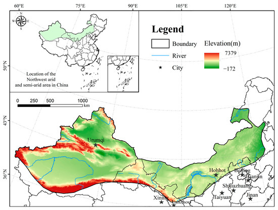
Figure 1.
Summary map of study area.
2.2. Data Acquisition and Pretreatment
2.2.1. NPP
Using MODIS (Moderate Resolution Imaging Spectroradiometer) data with a spatial resolution of 500 m, net primary productivity (NPP) products for the years 2001, 2005, 2010, 2015, and 2020 were obtained. These NPP products were derived from the EOS/MODIS TERRA satellite (MOD17A3H) provided by NASA in the United States. The data utilized an NPP estimation model established through the reference BIOME-BGC model and the light use efficiency model to simulate the annual NPP of terrestrial ecosystems. The pixel value represents the NPP value, indicating the sum of organic matter produced by photosynthesis throughout the year, minus the remaining portion after autotrophic respiration for the entire year [26]. The MODIS NPP products have undergone comprehensive evaluation and have been widely applied. Their spatiotemporal patterns are consistent with similar products from representative regions and periods worldwide [27,28,29,30,31,32].
2.2.2. Land Use
We utilized the MCD12Q1 land use product from MODIS with a spatial resolution of 500 m for the years 2001, 2005, 2010, 2015, and 2020. These datasets have been validated, and the overall accuracy reaches 75% [33], showing high consistency with other datasets, with an overall accuracy exceeding 70% [34,35,36]. Based on the latest land use classification methods and corresponding relationships, we have reclassified the data into six land use types: cropland, forestland, grassland, water bodies, urban areas, and unused land. The land use map of the study area for the year 2020 is shown in Figure 2.
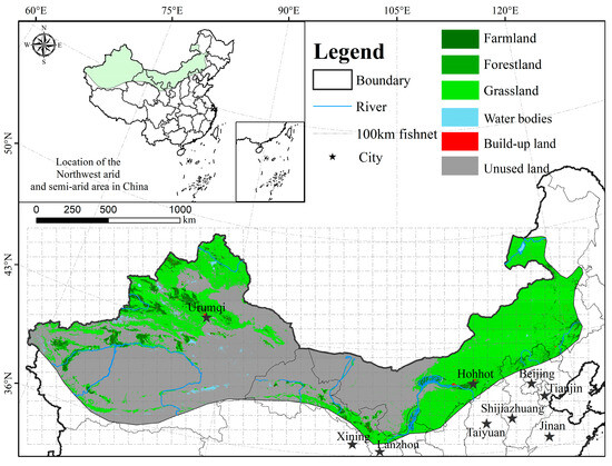
Figure 2.
Land use type map in arid and semi-arid regions of Northwest China in 2020.
2.3. Research Methods
2.3.1. Quadrat Selection
In order to better analyze the correlation between landscape patterns and NPP, this study employed the grid analysis method [37] based on previous research and the size of the study area. Five grid scales were selected: 50 km × 50 km, 80 km × 80 km, 100 km × 100 km, 120 km × 120 km, and 150 km × 150 km. These scales divided the study area into 1124, 471, 318, 231, and 153 grid units, respectively. To eliminate the influence of grid area on the results, grids with equal areas were selected, and grids with unequal areas were excluded for statistical analysis at the plot level. After conducting the analysis using Pearson correlation coefficients, the results indicated that the correlation coefficients depended on the spatial scale. The NPP and landscape indices showed the highest significance and correlation in the 100 km × 100 km grid units. Therefore, a spatial resolution of 100 km seems to be the optimal unit for this region.
2.3.2. Selection of Landscape Indicators
By using selected landscape indices and calculating these indices, one can quickly understand various landscape changes caused by factors such as natural environment and human activities. Choosing appropriate landscape indices allows for accurate and rapid assessment of the impact of environmental changes. The main advantages of landscape indices are their simplicity and speed of calculation as rapid environmental changes require easily obtainable indices. We used Fragstats 4.2 software to compute landscape indices [38,39]. In this study, considering the accuracy and effectiveness of analyzing the correlation between landscape patterns and NPP, we selected landscape indices from four categories: area and edge, size and heterogeneity, density, and aggregation [40]. These indices have been widely used in previous studies [41,42,43]. Area indices and edge indices reflect the number, size, and edge characteristics of patches. We chose Total Edge Length (TE) to quantify the percentage of patches in the total landscape area, representing landscape configuration and reflecting the complexity of patch shapes. We selected the Dispersed and Aggregated Index (IJI) to reflect the clustering trend between patches as a measure of landscape dispersion. Density index reflects the spatial pattern and heterogeneity of the landscape. We chose Number of Patches (NP) to describe the degree of fragmentation of the landscape. Diversity indices quantize the composition of the landscape at the landscape level, reflecting landscape heterogeneity. The Normalized Landscape Shape Index (NLSI) belongs to landscape shape indices and is capable of depicting the complexity of patch shapes. Consequently, it reflects the extent to which human activities influence the shape boundaries of that specific patch type. Therefore, we adopted the Shannon Diversity Index (SHDI) and Landscape Richness (PR) to quantify the composition of the landscape. NLSI belongs to landscape shape indices and can show changes in patch shapes. Therefore, we adopted the Shannon Diversity Index (SHDI) and Landscape Richness (PR) to quantify the composition of the landscape. NLSI (Normalized Landscape Shape Index) belongs to landscape shape indices and can show changes in patch shapes. Therefore, at the landscape level, we selected NP, TE, IJI, PR, and SHDI; at the class level, we selected NP, TE, IJI (Dispersed and Aggregated Index), and NLSI for calculation. The formulas for each index calculation are as follows:
where m represents the total number of patch types in the landscape; I represents a specific landscape patch type; pi represents the proportion of patch type i in the entire landscape. The ratio of pi landscape patch type i. SHDI reflects landscape heterogeneity and emphasizes the contribution of rare patch types [44]. Shannon diversity index is widely used to detect diversity in community ecology, which can reflect landscape heterogeneity, especially sensitive to the unbalanced distribution of patch types in the landscape. In addition, SHDI is also a sensitive indicator when comparing and analyzing the changes in diversity and heterogeneity in different landscapes or in different periods of the same landscape. For example, in a landscape system, the richer the land use is, the higher the degree of fragmentation is, the greater the information content of the step is, and the higher the calculated SHDI value is [44].
where represents the perimeter of the i-th landscape class, while denotes the perimeter of a circle with the same area. Patch shape index is the ratio of the shape of a patch to the circumference of a circle of the same area, which is used to describe the complexity of landscape patch shape. The larger the LSI value, the more complex the shape of the patch, and the greater the influence of human activities on the shape boundary of the patch type [44].
where N represents the total number of patches contained in a specific landscape patch type. The total number of patches in the landscape, NP ≥ 1. There is a good positive correlation between the total number of patches of a certain patch type in the landscape and the fragmentation of the landscape. Generally, NP is large, fragmentation is high, NP is small, and fragmentation is low [44].
where m is the total number of patches of a certain patch type, and eik is the total edge length between patch types i and k. When IJI value is small, it indicates that tile type i is only adjacent to a few other types; IJI = 100 indicates that the adjacent side lengths of each block are equal; that is, the adjacent probability of each block is equal. IJI is one of the most important indicators to describe the spatial pattern of landscape, and IJI reflects the distribution characteristics of ecosystems that are seriously restricted by some natural conditions. For example, various ecosystems in mountainous areas are seriously affected by vertical zonality, and their distribution is mostly annular, and IJI values are generally low. However, many transitional vegetation types in arid areas are subject to the distribution and abundance of water [44].
where the total length of all patch boundaries in the landscape [45].
where the total number of different patch types in the landscape, PR, is one of the key indicators to reflect the landscape components and spatial heterogeneity and has an impact on many ecological processes. It is found that there is a good positive correlation between landscape abundance and species abundance; especially for those organisms that need multiple habitat conditions for survival, PR is particularly important [45].
NP = N
TE = E
PR = M
2.3.3. Statistical Analysis
Previous studies have shown that landscape pattern is correlated with NPP, and the change in NPP is influenced by the change in landscape pattern [3,4]. In order to understand the influence of landscape pattern on NPP in detail, we determined the scale effect of the correlation between landscape pattern and NPP. Pearson correlation coefficient is used to calculate the relationship between landscape index and NPP in 100 km × 100 km grid scale, and the relationship between NPP and landscape index in 100 km grid scale is established by multiple linear regression method. Because of the large number of selected indicators, in order to show the high correlation between different indicators more clearly, this study chose the method of stepwise regression to reduce interference. The adjusted coefficient (R2) represents the prediction ability of multiple linear regression model, and the importance of different landscape pattern indexes is judged by standardized coefficient (Beta). The landscape index with high correlation with NPP was selected by SPSS 20 (p < 0.01) and a multiple linear regression model was established [46]. The preconditions for establishing a stepwise regression model are as follows: (1) the model adjustment coefficient (R2) after stepwise adjustment is the highest; (2) model coefficients and independent variables with significance less than or equal to 0.01; (3) the VIF value of each factor is less than 5. (VIF: variance expansion factor refers to the ratio of variance when there is multicollinearity between explanatory variables to variance when there is no multicollinearity. The value of VIF is greater than 1. The higher the value of VIF, the more serious the multicollinearity effect.)
where Y is the actual measured value, Xj is the independent variable, a0 is a constant, and ai is the partial regression coefficient, and then the normalized regression coefficient value is equal to aJ × (standard deviation of XJ/standard deviation of Y), and the positive and negative values of the normalized regression coefficient represent the positive and negative correlations, and the absolute values represent the degree of positive and negative correlations.
Y = a0 + a1X1 + a2X2 + … + ajXj + aJXJ
3. Results
3.1. Annual Change in NPP
Using the Zonal module in ArcMap 10.4, the NPP data for the study area from 2001 to 2020 were statistically analyzed, calculating the average NPP (Figure 3). The results show that, from 2001 to 2020, both the average and total net primary productivity of vegetation in the study area exhibited an increasing trend, and the trends were generally consistent. The NPP value was lowest in 2001 and reached its highest point in 2013. From 2001 to 2007, both the average and total NPP showed an initial increase followed by a decrease, with 2007 being the lowest value except for 2001. From 2007 to 2013, there was an upward trend, reaching a peak in 2013. From 2013 to 2020, the NPP values showed a fluctuating trend.
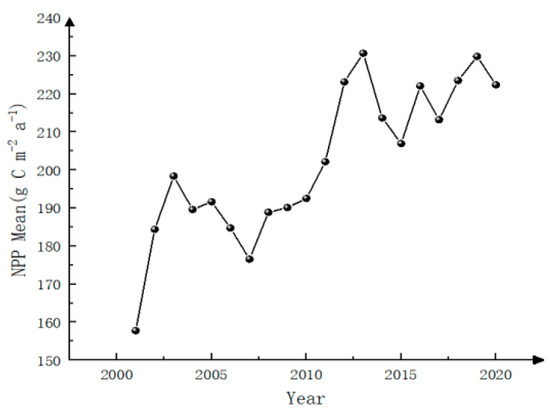
Figure 3.
Variation chart of NPP mean value from 2001 to 2020.
3.2. Spatial Distribution of NPP and Its Changing Characteristics
The spatial distribution of NPP in the study area over the past 20 years is shown in Figure 4. The high NPP values are concentrated in the northwest part of Xinjiang and the northeast part of Inner Mongolia, while the low NPP values are observed in the northwest part of Gansu and the central part of Inner Mongolia. The average NPP over the past 20 years reached 837.5 g C m2 a−1, with the lowest values found in the central region. Due to the prevalence of unused land and limited vegetation in the northwest arid and semi-arid regions, there are areas with NPP values of zero. From 2001 to 2020, the growth in NPP was primarily concentrated in the northeast part of Inner Mongolia, with the most significant increases observed near Jilin Province and Heilongjiang Province.
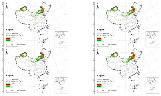
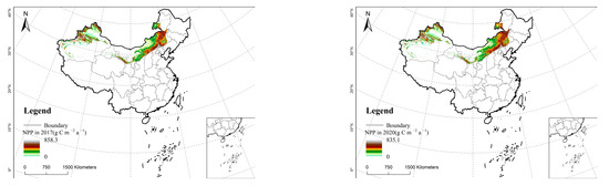
Figure 4.
Spatial variation in NPP from 2000 to 2020.
3.3. Changes in Landscape Pattern
3.3.1. Landscape Indicators at the Landscape Level
The changes in landscape indices at the landscape level from 2001 to 2020 are presented in the following table. The landscape indices were calculated at a 100 km grid scale, and the average values of each index across all grid scales are listed in Table 1 for the years 2001, 2005, 2010, 2015, and 2020. According to the table, over the 20-year period, the selected landscape indices at the landscape level, including NP, TE, IJI, PR, and SHDI, all show an increasing trend. NP increased from 146.60 in 2001 to 171.38 in 2020. TE increased from 14.42 to 16.28. IJI increased from 27.72 to 29.68. PR increased from 3.87 to 4.07. SHDI increased from 0.36 to 0.40. The fragmentation index NP reached its peak between 2015 and 2020, indicating the highest level of fragmentation in the northwest arid and semi-arid regions during that period. TE and IJI showed relatively gradual changes over the 20-year period. PR and SHDI increased annually, indicating an increase in both landscape richness and diversity in the study area over time.

Table 1.
Landscape-level landscape pattern index from 2001 to 2020.
3.3.2. Landscape Indicators at Class Level
The changes in landscape indices for different land use types, analyzed using Fragstats 4.2, are presented in Table 2, Table 3 and Table 4. For cropland, landscape indices NP and TE show a consistent increasing trend over the years, with a significant increase in magnitude. However, IJI shows a noticeable decreasing trend, while NLSI remains relatively stable. This indicates that the fragmentation of cropland landscapes has increased over the 20-year period, with a significant decline in connectivity between patches. In 2020, the cropland landscape in the study area shows poorer connectivity compared to 2001. For forestland, NP and TE show an increasing trend, while IJI shows a decreasing trend over the years. This indicates a similar pattern of changes in forestland patches as observed for cropland: an increase in fragmentation and a decline in connectivity between forest patches. For grassland, NP and TE initially decrease and then increase, while IJI shows an increasing trend. The fragmentation of grassland in the study area decreased from 2005 to 2010 but has been gradually increasing since then. The connectivity of grassland patches has gradually increased over the 20-year period. Cropland and forestland have a higher number of patches, while grassland shows a higher connectivity index percentage. This is related to the respective areas of land use types: cropland and grassland have larger areas compared to forestland. Grassland exhibits better connectivity compared to cropland and forestland. Overall, these results indicate that cropland and forestland in the study area have become more fragmented over the 20-year period, while grassland has shown fluctuations in fragmentation and improved connectivity.
Table 2.
Interannual change in landscape pattern index at class level (Farmland).
Table 3.
Interannual change in landscape pattern index at class level (Forestland).
Table 4.
Interannual change in landscape pattern index at class level (Grassland).
3.4. Study on the Correlation between NPP and Landscape Index
3.4.1. Landscape Level
As shown in Table 5, the majority of regressions are significant at the 0.01 level, while a few regressions are significant at the 0.1 level. All landscape indices exhibit a strong positive correlation with NPP. The correlations between IJI and SHDI with NPP show a decreasing trend over the 20-year period, indicating a decreasing correlation between NPP and IJI/SHDI over time. NP, TE, and PR show relatively small fluctuations without significant changes. Among them, PR has the strongest correlation with NPP, followed by NP, indicating that higher landscape richness is associated with higher NPP values, and higher fragmentation is also associated with higher NPP values. To identify the most important landscape indices in explaining variation in NPP, a stepwise selection of landscape indices was conducted using multiple linear regression. At the landscape level, the multiple linear regression model of NPP and landscape index at the 100 km grid scale in 2020 is NPP = 0.617 × NP + 0.454 × PR − 0.599 × SHDI (R2 = 0.454, p < 0.01). The results demonstrate a clear linear relationship between NPP and landscape indices. The multiple linear regression model shows that NP, PR, and SHDI explain 45.4% of the variation in vegetation net primary productivity. NP and PR have positive effects on NPP, while SHDI has a negative effect. In the model, the standardized coefficient for NP is 0.617, for PR 0.454, and for SHDI 0.599, indicating that all three landscape pattern indices have a relatively high impact on NPP.
Table 5.
Correlation between NPP and landscape index from 2000 to 2020.
3.4.2. Class Level
The correlation between landscape indices and NPP for different land use types is shown in Table 6. In croplands, forests, and grasslands, the landscape indices exhibit a strong and significant correlation with NPP. However, in unused land and urban areas, where NPP values are generally low, the correlation with landscape indices is weaker and often insignificant. In croplands, except for NLSI, all other indices show a strong positive correlation with NPP. Among them, TE, which represents edge characteristics, NP, which represents patch density, and IJI, which represents aggregation trend, exhibit a strong positive correlation with NPP, and the correlation is highly significant at the 0.01 level. NP shows the highest correlation with NPP (0.729). In forests, all four landscape indices show a strong positive correlation with NPP, and the correlation is highly significant at the 0.1 level. In grasslands, TE and IJI exhibit a strong correlation with NPP, while NLSI and NP have a low and insignificant correlation. Overall, grassland landscape indices are relatively lower compared to croplands and forests. In urban areas, NLSI shows a strong correlation with NPP, while, in unused land, NP shows a strong correlation with NPP. In summary, in croplands and forests, fragmented landscape types are associated with higher NPP values, and greater proximity between patches is also associated with higher NPP values. However, in croplands, higher complexity in patch shape is associated with lower NPP values, while, in forests, this relationship is not significant. Table 7 shows the multiple linear regression equations calculated for different land use types. The model parameters differ for different land use types. Since water bodies have low NPP values, they are not discussed at the class level. In the cropland regression model, NP and TE explain 67.4% of the variation in NPP, and both indices have a positive impact on NPP. NP plays a more important role in explaining NPP increase in croplands compared to other landscape indices. In the forest regression model, the relationship between NPP and IJI is more significant, and IJI is the most effective index in explaining NPP increase. In the grassland regression model, TE, IJI, and NP explain 73.1% of the variation in NPP. TE and IJI have a positive effect on NPP, while NP has a negative effect. The regression models for croplands, forests, and grasslands show that the main landscape indices explaining the variation in NPP differ for these land use types. The beta coefficients in the models for urban areas and unused land indicate that NP plays the most important role in explaining NPP increase in these land use types. In the unused land regression model, these indices contribute the least to explaining the variation in NPP, possibly due to the low NPP values in unused land, which makes it difficult to obtain significant results. The results demonstrate that the relationship between landscape pattern and NPP is more favorable for analysis when considering different land use types.
Table 6.
Correlation between class-level landscape indicators and NPP.
Table 7.
The class-level multiple linear regression equation of landscape index and NPP.
4. Discussion
4.1. Impact of Landscape Pattern on NPP
In previous studies, the significant correlation between landscape indices and NPP reflects the important influence of landscape pattern changes on regional vegetation NPP [40], with the fundamental cause of landscape pattern changes being land use change [40]. Rapid population growth, migration, urbanization, and social development are major influencing factors [47], which align with the results of this study. Late-20th-century immigration projects [48] increased the area of population, cultivated land, and urban land while decreasing forested areas [49]. The increase in human-modified landscapes also adversely affected the vegetation patterns of the study area. Since the last century, ecological construction projects such as “Grain for Green” and “Three-North Shelterbelt Program” implemented by the Chinese government have been another important factor in landscape pattern changes in the arid and semi-arid regions of Northwest China. These projects have played a crucial role in vegetation and ecosystem restoration in China [50]. Human activities influence landscape patterns through land use changes, and, in the arid and semi-arid areas of Northwest China, human activities are primarily reflected in some level of grazing. From 2001 to 2010, the livestock population in Inner Mongolia increased significantly, reaching 30 million heads, leading to increased grazing pressure and accelerated grassland degradation, subsequently affecting NPP [51]. The “Grazing Withdrawal program” proposed in the last century emphasizes the restoration of degraded grasslands by reducing grazing intensity. The implementation of this program has transformed some unused land into grasslands in certain areas within the study area [51,52]. With the initiation of the program, grazing pressure has decreased. For example, in the Alashan Desert Grassland, after a long period of grazing prohibition, grass biomass significantly increased, leading to an increase in vegetation net primary productivity in the region [53]. Restraining grazing during specific periods is also considered necessary [54]. From the late 20th century to the early 21st century, taking some cities in Gansu Province located in the arid and semi-arid regions of Northwest China as an example, due to rapid population growth and economic development, the area of cultivated land has been decreasing over the course of 20 years [55]. Similarly, in the southern part of Xinjiang Uygur Autonomous Region, also situated in the arid and semi-arid regions of Northwest China, the population growth rate has been 30.3% since the beginning of the 21st century, leading to significant land development and urbanization [56]. Rapid population growth and accelerated urbanization have affected land use types and distribution, resulting in lower NPP values in Gansu Province and southern Xinjiang. In Inner Mongolia, since 2005, the implementation of projects such as the “Grain for Green Project” and the “Beijing-Tianjin Sand Source Control Project” has endowed the grassland and forests in the region with high ecological service value [57], and the areas of forests and grasslands have remained relatively stable. Furthermore, between 2000 and 2019, the temperature and precipitation conditions in Inner Mongolia’s northeast were slightly better compared to other regions in the arid and semi-arid regions of Northwest China [58], which explains the higher NPP values in the northeastern part of Inner Mongolia. Table 8 presents the land use transition matrix for the study area of Northwest China from 2001 to 2020. The land use transition matrix is used to clearly express the changes in the area of each land use type over the 20-year period. From the land use transition matrix, it can be observed that, except for water bodies, all other land use types have undergone significant changes. Over the course of 20 years, 36,515.51 km2 of grassland was converted into cultivated land, while 8735.64 km2 was converted into unused land. Additionally, 9911.24 km2 of cultivated land was converted into grassland, and 974.82 km2 of forested land was converted into grassland. The mutual conversion of areas between cultivated land, forest, and grassland has led to changes in NPP values. Furthermore, with the increasing demand for food production due to population growth, cultivated land resources have become increasingly limited, leading to higher demand for agricultural products and fertilizers. This has driven the effective output of cultivated land resources, increasing net primary productivity per unit area. Overall, the implementation of ecological engineering has had a significant impact on the landscape pattern and net primary productivity of the study area. The spatial correlation between landscape pattern and NPP should be provided due attention.
Table 8.
Land use transfer matrix in arid and semi-arid regions of Northwest China from 2001 to 2020. Unit: km2.
4.2. Selection of Landscape Index and Determination of Spatial Scale
Landscape indices are typically selected based on the characteristics of the indices themselves [59,60]. As mentioned earlier, landscape indices can be categorized into four major groups: area and edge, shape, aggregation, and diversity. While there are numerous and diverse landscape indices to choose from, they can provide overlapping information. Therefore, in this study, we used a combination of multiple linear regression equations and the VIF to select indices in order to reduce overlap. The results of the multiple linear regression equation reveal which indices have a significant impact on NPP under different landscape categories, allowing for targeted addition of landscape types to enhance NPP. The choice of scale is another important aspect of landscape pattern research as it directly affects the accuracy and reliability of the results [61]. In landscape ecology, scale mainly refers to the role of spatiotemporal granularity, with a focus on spatial scale and spatial heterogeneity. Spatial heterogeneity is a fundamental characteristic of landscapes, and scale heterogeneity is an inherent feature of spatial heterogeneity [62]. Previous studies have shown that SHDI increases over time, and the magnitude of increase does not change with the coarsening of grains; NP shows fewer inflection points and increases with the enlargement of grain size. In this study, NP rises from 146.6 to 171.38, while SHDI continues to increase from 0.36 to 0.4, consistent with previous research [63,64]. Over the past 20 years, increase in landscape spatial heterogeneity may be related to the formation of afforestation belts, increase in the number of young forests, and quality [24]. The formation of green belts increases landscape diversity, and young forests are vibrant, with higher NPP. In the past 20 years, the level of fragmentation in the study area has gradually increased, which is inconsistent with the research results of Zhao et al., 2018 [3] (with no significant change in fragmentation level) and Zhang et al.,2020a [65] (with significant reduction in fragmentation level). This difference may be related to the fact that the formation of afforestation belts and the growth of young forests do not necessarily change the level of landscape fragmentation. The increase in IJI in the study area may be due to the continuity between newly formed afforestation belts and newly grown young forests and natural forests, leading to increased connectivity over time. NP is positively correlated with NPP, indicating that, as the number of patches and the degree of fragmentation increase, NPP values also increase. SHDI and PR are positively correlated with NPP, suggesting that, as landscape diversity increases, NPP values also increase. IJI is positively correlated with NPP, indicating that, as patch connectivity increases, net primary productivity increases. The individual landscape pattern indices calculated in this study show a relatively weak correlation with NPP. For instance, at the landscape level, SHDI has a low correlation with NPP. At the class level, the number of patches for grassland (NP), total edge length for unused land (TE), and dispersion and juxtaposition index for built-up land (IJI) also exhibit weak correlations with NPP. This may be attributed to the relatively low data resolution used in the study. Since the 21st century, China’s ecological conservation projects have begun to show results, leading to an increase in landscape diversity, improvement in connectivity, an increase in the number of patches, and a continued increase in landscape fragmentation. However, in the arid and semi-arid regions of Northwest China, the distribution of NPP and landscape patterns remains uneven, especially in the northeastern part of Inner Mongolia and the northern part of Xinjiang, where NPP is higher, while the northern part of Gansu has lower NPP. In the northeastern part of Inner Mongolia, the construction of ecological projects and the presence of large areas of forests and grasslands have resulted in significantly higher patch connectivity compared to Gansu Province, where forests and grasslands are scarce. Therefore, when implementing ecological conservation projects such as “Grain for Green”, priority should be given to regions with severe forest resource scarcity and harsh climate conditions, with a focus on restoring landscape diversity and improving landscape structure to achieve sustainable development of regional ecology and society.
4.3. Research Limitations and Prospects
The shortcomings in this study have important implications for the management and monitoring of ecological environments. First, although the land use data and NPP data based on MODIS that we selected have been validated and are reliable, the low resolution of the data may lead to deviations in the results, and there may be differences between NPP products and model-estimated NPP. In the future, higher-resolution data can be used for further research. Additionally, remote sensing data have attributes such as spatial and temporal resolutions, and addressing the trade-off between resolutions is another issue to be resolved. Second, the time interval of this study was set at 5 years from 2000 to 2020. In future studies, it would be beneficial to refine the time interval and use continuous time series to study the correlation. Third, we selected a small number of indices in the study to reduce redundancy and chose representative indices to quantify the relationship between NPP and landscape pattern. However, there may be other unselected indices that may provide greater accuracy. Therefore, a comprehensive landscape index is needed to integrate the composition of landscape patterns. In arid regions, climate conditions are crucial factors in ecological research and management. The unique arid climate, sparse precipitation, and sparse vegetation create unique ecological environments. Extreme climate conditions affect temperature, precipitation, and vegetation growth, ultimately changing the landscape pattern. However, it is not sufficient to only explore the relationship between climate change and landscape pattern. In the future, further research will be conducted on the relationship between climate change, vegetation growth, and landscape pattern changes. Overall, the above research results are of great significance, and they provide valuable directions for future research to enhance the understanding of the correlation between landscape pattern changes and NPP in the northwest arid and semi-arid regions. Considering data resolution, time intervals, index selection, and climate factors will help to better understand and explain the impact of landscape pattern changes on NPP in ecosystems, providing more effective guidance and decision support for ecological environment management and monitoring.
5. Conclusions
In the arid and semi-arid regions of Northwest China, the overall trend in vegetation net primary productivity (NPP) has shown an increase over the past 20 years. High NPP values are primarily concentrated in the northeastern part of Inner Mongolia and the northern part of Xinjiang, while Gansu Province is characterized by low values. The spatial variation in NPP is not only related to land use type changes in the study area but also influenced by factors such as crop yield, which affect the vegetation’s carbon sequestration capacity. From the perspective of landscape pattern, different landscape types are influenced by different factors, leading to variations in NPP. Increases in landscape fragmentation, diversity, and aggregation will all contribute to an increase in NPP. Therefore, during landscape pattern optimization and ecological environment management, different landscape types contribute to NPP to varying degrees, and their carbon sequestration capacities differ as well. Only by setting up appropriate landscape types can regional NPP growth be promoted. Thus, rational planning of landscape types can create opportunities for NPP growth. These research findings provide valuable suggestions for optimizing landscape patterns.
Author Contributions
Data curation, C.X.; Software, C.X.; Writing original draft, C.X.; Conceptualization, C.L.; Methodology, C.L.; Supervision, C.L. All authors have read and agreed to the published version of the manuscript.
Funding
This research was funded by National Natural Science Foundation Project: Effects of relative climate change on net primary productivity of vegetation: a case study in arid Northwest China, grant number 42161058.
Data Availability Statement
The new data created in this study are available on request.
Conflicts of Interest
The authors declare no conflict of interest.
References
- Turner, M.; Ruscher, C. Changes in landscape patterns in Georgia, USA. Landsc. Ecol. 1998, 1, 241–251. [Google Scholar] [CrossRef]
- Uuemaa, E.; Mander, Ü.; Marja, R. Trends in the use of landscape spatial metrics as landscape indicators: A review. Ecol. Indic. 2013, 28, 100–106. [Google Scholar] [CrossRef]
- Zhao, X.; Zhou, W.; Tian, L.; He, W.; Zhang, J.; Liu, D.; Yang, F. Effects of land-use changes on vegetation net primary productivity in the Three Gorges Reservoir Area of Chongqing. Acta Ecol. Sinica. 2018, 38, 7658–7668. [Google Scholar]
- Cheng, F.; Liu, S.; Zhang, Y.; Yin, Y.; Hou, X. Effects of land use change on net primary productivity in Beijing based on MODIS series. Acta Ecol. Sinica. 2017, 37, 5924–5934. [Google Scholar]
- Frondoni, R.; Mollo, B.; Capotorti, G. A landscape analysis of land cover change in the Municipality of Rome (Italy): Spatiotemporal characteristics and ecological implications of land cover transitions from 1954 to 2001. Landsc. Urban Plan 2011, 100, 117–128. [Google Scholar] [CrossRef]
- Groot, R.; Brander, L.; Ploeg, S.; Costanza, R.; Bernard, F.; Braat, L.; Christie, M.; Crossman, N.; Ghemandi, A.; Hein, L.; et al. Global estimates of the value of ecosystemsand their services in monetary unit. Ecosyst. Serv. 2012, 1, 50–61. [Google Scholar] [CrossRef]
- Field, B.; Behrenfeld, J.; Randerson, T.; Paul, F. Primary production of the biosphere: Integrating terrestrial and oceanic components. Science 1998, 281, 237–240. [Google Scholar] [CrossRef] [PubMed]
- Bai, Z.; Dent, D.; Olsson, L.; Schaepman, M. Proxy global assessment of land degradation. Soil Use Manag. 2008, 24, 223–234. [Google Scholar] [CrossRef]
- Li, J.; Wang, Z.; Lai, C. Severe drought events inducing large decrease of net primary productivity in mainland China during 1982–2015. Sci. Total Environ. 2020, 703, 135541. [Google Scholar] [CrossRef]
- Hu, Y.; Jia, G.; Guo, H. Linking primary production, climate and land use along an urban–wildland transect: A satellite view. Env. Rese Lett. 2009, 4, 044009. [Google Scholar] [CrossRef]
- Yang, Y.; Guan, H.; Batelaan, O.; McVicar, T.; Long, D.; Pao, S.; Liang, W.; Liu, B.; Jin, Z.; Simmons, C.T. Contrasting responses of water use effciency to drought across global terrestrial ecosystems. Sci. Rep. 2016, 6, 23284. [Google Scholar] [CrossRef] [PubMed]
- Zhou, W.; Gang, C.; Zhou, F.; Li, J.; Dong, X.; Zhao, C. Quantitative assessment of the individual contribution of climate and human factors to desertification in northwest China using net primary productivity as an indicator. Ecol. Indic. 2015, 48, 560–569. [Google Scholar] [CrossRef]
- Zheng, Y.; Xie, Z.; Robert, C.; Jiang, L.; Shimizu, H. Did climate drive ecosystem change and induce desertification in Otindag sandy land, China over the past 40 years? J. Arid Environ. 2006, 64, 523–541. [Google Scholar] [CrossRef]
- Wessels, K.J.; Prince, S.D.; Reshef, I. Mapping land degradation by comparison of vegetation production to spatially derived estimates of potential production. J. Arid Environ. 2008, 72, 1940–1949. [Google Scholar] [CrossRef]
- Li, W.; Li, C.; Liu, X.; He, D.; Bao, A.; Yi, Q.; Wang, B.; Liu, T. Analysis of spatial–temporal variation in NPP based on hydrothermal conditions in the Lancang-Mekong River Basin from 2000 to 2014. Env. Monit Assess 2018, 190, 321–335. [Google Scholar] [CrossRef]
- Chen, A.; Yao, L.; Sun, R.; Chen, L. How many metrics are required to identify the effects of the landscape pattern on land surface temperature? Ecol. Indic. 2014, 45, 424–433. [Google Scholar] [CrossRef]
- Yan, Y.; Liu, X.; Wen, Y.; Ou, J. Quantitative analysis of the contributions of climatic and human factors to grassland productivity in northern China. Ecol. Indic. 2019, 103, 542–553. [Google Scholar] [CrossRef]
- Wu, S.; Zhou, S.; Chen, D.; Wei, Z.; Dai, L.; Li, X. Determining the contributions of urbanisation and climate change to NPP variations over the last decade in the Yangtze River Delta, China. Sci. Total Environ. 2014, 472, 397–406. [Google Scholar] [CrossRef]
- Zhang, Y.; Song, C.; Zhang, K.; Cheng, X.; Band, L.; Zhang, Q. Effects of land use/land cover and climate changes on terrestrial net primary productivity in the Yangtze River Basin, China, from 2001 to 2010. J. Geophys. Res. Biogeosci. 2014, 119, 1092–1109. [Google Scholar] [CrossRef]
- DeFries, R.; Field, C.; Fung, I.; Collatz, G.; Bounoua, L. Combined satellite data and biogeochemical models to estimate global effects of human—Induced land cover change on carbon emissions and primary productivity. Glob. Biogeochem. 1999, 13, 803–815. [Google Scholar] [CrossRef]
- Milesi, C.; Elvidge, C.D.; Nemani, R.R.; Running, S.W. Assessing the impact of urban land development on net primary productivity in the southeastern United States. Remote Sens. Environ. 2003, 86, 401–410. [Google Scholar] [CrossRef]
- McGarigal, K.; Cushman, S.; Maile, N.; Ene, E. FRAGSTATS: Spatial Pattern Analysis for Categorical Maps. Comput. Softw. Progr. Prod. 2002. [Google Scholar]
- Cushman, S.; McGarigal, K.; Neel, M. Parsimony in landscape metrics: Strength, universality, and consistency. Ecol. Indic. 2008, 8, 691–703. [Google Scholar] [CrossRef]
- Lustig, A.; Stouffer, D.; Roigé, M.; Worner, S. Towards more predictable and consistent landscape metrics across spatial scales. Ecol. Indic. 2015, 57, 11–21. [Google Scholar] [CrossRef]
- Ye, F. Application of multiple linear regression in economic and technical output forecasting. China Foreign Energy 2015, 2, 45–48. [Google Scholar]
- Jiang, R.; Li, X.; Zhu, Y.; Zhang, Z. Spatial and temporal variation of NPP and NDVI correlation in the Yellow River Delta wetland based on MODIS. Acta Ecol. Sinica. 2011, 31, 6708–6716. [Google Scholar]
- Turner, D.P.; Ritts, W.D.; Cohen, W.B. Evaluation of modis NPP and GPP products across multiple biomes. Remote Sens. Env. Ment. 2006, 102, 282–292. [Google Scholar] [CrossRef]
- Turner, D.P.; Ritts, W.D.; Zhao, M. Assessing interannual variation in modis-based estimates of gross primary production. IEEE Trans. Geosci. Remote Sens. 2006, 44, 1899–1907. [Google Scholar] [CrossRef]
- Zhao, M.; Running, S.W. Drought-induced reduction in global terrestrial net primary production from 2000 through 2009. Science 2010, 329, 940–943. [Google Scholar] [CrossRef]
- Hasenauer, H.; Petritsch, R.; Zhao, M. Reconciling satellite with ground data to estimate forest productivity at national scales. For. Ecol. Manag. 2012, 276, 196–208. [Google Scholar] [CrossRef]
- Bastos, A.; Running, S.W.; Gouveia, C. The global NPP dependence on ENSO: La-Niña and the extraordinary year of 2011. J. Geophys. Res. Biogeosciences 2013, 118, 1247–1255. [Google Scholar] [CrossRef]
- Zhao, M.; Running, S.W.; Nemani, R.R. Sensitivity of moderate resolution imaging spectroradiometer (MODIS) terrestrial primary produc-tion to the accuracy of meteorological reanalyses. J. Geophys Ical Res. 2015, 111, 338–356. [Google Scholar]
- Friedl, M.A.; Sulla-Menashe, D.; Tan, B. Modis collection 5 global land cover: Algorithm refinements and characterization of new datasets. Remote Sens. Environ. 2010, 114, 168–182. [Google Scholar] [CrossRef]
- Liang, D.; Zuo, Y.; Huang, L. Evaluation of the consistency of modis land cover product (MCD12Q1) based on Chinese 30 m globeland30 datasets: A case study in Anhui Province, China. ISPRS Int. J. Geo-Inf. 2015, 4, 2519–2541. [Google Scholar] [CrossRef]
- Cao, C.; Lee, X.; Liu, S. Urban heat islands in China enhanced by haze pollution. Nat. Commun. 2016, 7, 12509. [Google Scholar] [CrossRef] [PubMed]
- Yang, K.; Xiao, P.; Feng, X. Accuracy assessment of seven global land cover datasets over China. ISPRS J. Photogramme-Try Remote Sens. 2017, 125, 156–173. [Google Scholar] [CrossRef]
- Chang, Y.; Gao, Y.; Xie, Z. Relationship between habitat quality and landscape pattern evolution in Beijing-Tianjin-Hebei region. Chin. J. Environ. Sci. 2021, 201, 848–859. [Google Scholar]
- McGarigal, K.; Cushman, S.; Maile, N.; Ene, E. Fragstats V4: Spatial Pattern Analysis Program for Categorical and Continuous Maps. Comput. Softw. Progr. Prod. 2012. [Google Scholar]
- Feng, Y.; Liu, Y.; Tong, X. Spatiotemporal variation of landscape patterns and their spatial determinants in Shanghai. Ecol. Indic. 2018, 87, 22–32. [Google Scholar] [CrossRef]
- Ayinuer, Y.; Zhang, F.; Yu, H.; Kung, H. Quantifying the spatial correlations between landscape pattern and ecosystem service value: A case study in Ebinur Lake Basin, Xinjiang, China. Ecol. Eng. 2018, 113, 94–104. [Google Scholar]
- Schindler, S.; Poirazidis, K.; Wrbka, T. Towards a core set of landscape metrics for biodiversity assessments: A case study from Dadia National Park, Greece. Ecol. Indic. 2008, 8, 502–514. [Google Scholar] [CrossRef]
- Kumar, M.; Denis, D.; Singh, S.; Szabó, S.; Suryavanshi, S. Landscape metrics for assessment of land cover change and fragmentation of a heterogeneous watershed. Remote Sens. Appl. Soc. Environ. 2018, 10, 224–233. [Google Scholar] [CrossRef]
- Jia, Y.; Tang, L.; Xu, M.; Yang, X. Landscape pattern indices for evaluating urban spatial morphology-A case study of Chinese cities. Ecol. Indic. 2019, 99, 27–37. [Google Scholar] [CrossRef]
- Feng, Z. Analysis of Landscape Pattern and Its Influencing Factors in Yilong Lake Basin. Master’s Thesis, Yunnan Normal University, Kunming, China, 2021. [Google Scholar]
- Zhou, Y.; Yue, D.; Guo, J.; Chen, G.; Wang, D. Spatial correlations between landscape patterns and net primary productivity: A case study of the Shule River Basin, China. Ecol. Indic. 2021, 130, 108067. [Google Scholar] [CrossRef]
- Xu, S.; Li, S.; Zhong, J.; Li, C. Spatial scale effects of the variable relationships between landscape pattern and water quality: Example from an agricultural karst river basin, Southwestern China. Agric. Ecosyst. Environ. 2020, 300, 106999. [Google Scholar] [CrossRef]
- Liu, J.; Linderman, M.; Ouyang, Z.; An, L.; Yang, J.; Zhang, H. Ecological bai degradation in protected areas: The case of Wolong nature reserve for giant pandas. Science 2001, 292, 98–101. [Google Scholar] [CrossRef] [PubMed]
- Ma, L.; Bo, J.; Li, X.; Fang, F.; Cheng, W. Identifying key landscape pattern indices influencing the ecological security of inland river basin: The middle and lower reaches of Shule River Basin as an example. Sci. Total Environ. 2019, 674, 424–438. [Google Scholar] [CrossRef] [PubMed]
- Song, X.; Yan, C.; Li, S.; Xie, J. Assessment of sandy desertification trends in the Shule River Basin from 1978 to 2010. Sci. Cold Arid Reg. 2014, 16, 52–58. [Google Scholar]
- Chen, C.; Park, T.; Wang, X.; Piao, S.; Xu, B.; Chaturvedi, R.; Fuchs, R.; Brovkin, V.; Ciais, P.; Fensholt, R.; et al. China and India lead in greening of the world through land-use management. Nat. Sustain. 2019, 2, 122–129. [Google Scholar] [CrossRef] [PubMed]
- Mu, S.; Zhou, S.; Chen, Y.; Li, J.; Ju, W.; Odeh, I.O.A. Assessing the impact of restoration-induced land conversion and management alternatives on net primary productivity in Inner Mongolian grassland. China. Glob. Planet. Chang. 2013, 108, 29–41. [Google Scholar] [CrossRef]
- Zhang, Y.; Zhang, C.; Wang, Z.; Chen, Y.; Gang, C.; An, R.; Li, J. Vegetation dynamics and its driving forces from climate change and human activities in the Three-River Source Region, China from 1982 to 2012. Sci. Total Environ. 2016, 563–564, 210–220. [Google Scholar] [CrossRef] [PubMed]
- Pei, S.; Fu, H.; Wan, C. Changes in soil properties and vegetation following exclosure and grazing in degraded Alxa desert steppe of Inner Mongolia, China. Agric. Ecosyst. Environ. 2008, 124, 33–39. [Google Scholar] [CrossRef]
- Gao, J.; Liu, Y. Determination of land degradation causes in Tongyu County, Northeast China via land cover change detection. Int. J. Appl. Earth Obs. Geoinf. 2010, 12, 9–16. [Google Scholar] [CrossRef]
- Wang, H.; Ma, Q.; Fu, S.; Han, N. Study on the correlation between cultivated land area change and population and economic development in arid and semi-arid region of Northwest China—A case study of Gansu Province. J. Arid. Land Resour. Environment. 2011, 25, 36. [Google Scholar]
- Mirzatijan, M.; Gulmi, E.; Ayitulsun, S. Spatial-temporal change and driving factors of land use/cover in Xinjiang based on MODIS data. Hubei Agric. Sci. 2022, 61, 58–63. [Google Scholar]
- Wang, N.; Yang, G. Land use change and ecosystem service value in Inner Mongolia, 1990–2018. J. Soil Water Conserv. 2022, 34, 244–250. [Google Scholar]
- Zhang, Z.; Xiong, M.; Li, F.; Liu, X.; Hao, Y.; Xing, L.; Wang, X.; Lai, M.; Yuan, P. Analysis of the temporal and spatial variations in net primary productivity of vegetation in the grassland region of Inner Mongolia and the factors influencing those changes. Pratacultural Sci. 2022, 39, 2492–2502. [Google Scholar]
- Estreguil, C.; De Rigo, D.; Caudullo, G. A proposal for an integrated modelling framework to characterise habitat pattern. Environ. Modell. Softw. 2014, 52, 176–191. [Google Scholar] [CrossRef]
- Feng, Y.; Liu, Y. Fractal dimension as an indicator for quantifying the effects of changing spatial scales on landscape metrics. Ecol. Indic. 2015, 53, 18–27. [Google Scholar] [CrossRef]
- Gustafson, E. Quantifying landscape spatial pattern: What is the state of the art? Ecosystems 1998, 1, 143–156. [Google Scholar] [CrossRef]
- Wu, J.; Jelinski, D.; Luck, M.; Tueller, P. Multiscale analysis of landscape heterogeneity: Scale variance and pattern metrics. Ann. Gis. 2000, 6, 6–19. [Google Scholar] [CrossRef]
- Chen, Y. Responses of Forest Productivity and Carbon Storage to Landscape Pattern Change in the Three Gorges Reservoir Area; Chinese Academy of Forestry Sciences: Beijing, China, 2017. [Google Scholar]
- Zhu, M.; Pu, L.; Li, J. The influence of spatial resolution and grain size change of remote sensing image on urban landscape pattern analysis. Acta Ecol. Sinica. 2008, 28, 2753–2763. [Google Scholar]
- Zhang, Q.; Chen, C.; Wang, J.; Yang, D.; Zhang, Y.; Wang, Z.; Gao, M. The spatial granularity effect, changing landscape patterns, and suitable landscape metrics in the Three Gorges Reservoir Area, 1995–2015. Ecol. Indic. 2020, 114, 106259. [Google Scholar] [CrossRef]
Disclaimer/Publisher’s Note: The statements, opinions and data contained in all publications are solely those of the individual author(s) and contributor(s) and not of MDPI and/or the editor(s). MDPI and/or the editor(s) disclaim responsibility for any injury to people or property resulting from any ideas, methods, instructions or products referred to in the content. |
© 2023 by the authors. Licensee MDPI, Basel, Switzerland. This article is an open access article distributed under the terms and conditions of the Creative Commons Attribution (CC BY) license (https://creativecommons.org/licenses/by/4.0/).