Spatiotemporal Changes in Water Storage and Its Driving Factors in the Three-River Headwaters Region, Qinghai–Tibet Plateau

Abstract

Water storage (WS) is a crucial terrestrial ecosystems service function. In cold alpine regions (CAR), the cryosphere elements are important solid water resources, but the existing methods for quantitatively assessing WS usually ignore cryosphere elements. In this study, a revised Seasonal Water Yield model (SWY) in the Integrated Valuation of Ecosystem Services and Trade-offs (InVEST), which considers the effects of frozen ground (FG) and snow cover (SC) on WS, was employed to estimate the spatiotemporal distribution and changes in WS in the Three-Rivers Headwaters region (TRHR) from 1981 to 2020. Sensitivity analyses were conducted to understand the overall effects of multiple factors on WS, as well as the dominant driving factors of WS change at the grid scale in the TRHR. The results show that (1) the WS in the TRHR generally increased from 1981 to 2020 (0.56 mm/year), but the spatial distribution of WS change varied greatly, with a significant increasing trend in the northwest part and a significant decreasing trend in the southeast part. (2) In the last 40 years, increased precipitation (Pre) positively affected WS, while increased potential evapotranspiration (ET₀) reduced it. Increased permeability caused by degradation of frozen ground increased WS, while snow cover and LULC changes reduced it. (3) In the TRHR, Pre primarily affected the WS with the largest area ratio (32.62%), followed by land use/land cover (LULC) (19.69%) and ET₀ (18.49%), with FG being fourth (17.05%) and SC being the least (6.64%). (4) The highly important and extremely important zones generally showed a decreasing trend in WS and should be treated as key and priority conservation regions. It is expected that this research could provide a scientific reference for water management in the TRHR.

1. Introduction

Water-related ecosystem services information is important in the realm of water management and decision making [1,2,3,4]. Water storage (WS) refers to the mechanism and capacity of ecosystems regarding the interception, infiltration, and storage of precipitation (Pre) within a specific spatiotemporal scope [5,6]. This enables the fulfillment of internal water requisites while also furnishing invaluable water resources to external regions, including downstream regions [5,6,7]. WS holds a vital position among the myriad of ecosystems services, standing as a pivotal indicator reflecting the state of ecosystems. WS change (WSC) not only wields a direct influence over the condition of natural elements within a watershed and the processes of the ecosystem but yields an influence on the ecosystems and water resources of downstream regions indirectly [6,8]. Consequently, quantitatively assessing the WSC of ecosystems, understanding the relationship between WSC and ecosystem processes and human activities in different regions, and conducting spatial division of WS importance are of great practical significance for optimizing ecological barriers, addressing climate change risks, and optimizing water resource allocation in downstream areas [9]. Moreover, they provide crucial guidance for regional sustainable development [9].

The methods for quantitatively assessing WS have evolved in accordance with the comprehension of its significance. Prior to the 1980s, scholars embarked on investigating the effect of forest ecosystems on water yield (increment or decrement) through field experiments [10]. However, the concept of WS was not clear at this stage. In the 1980s, the concept of WS in forest ecosystems was gradually clarified. Numerous methods for estimating WS emerged, predominantly using observation data to estimate the amount of water held by different layers of forest by simple arithmetic operations [11,12,13,14]. Nevertheless, these methods omitted the hydrophysical processes. In the past decade, scholars have gradually adopted modeling methods to comprehensively assess the function of WS, and the concept of WS has gradually been enriched and hydrophysical processes have been considered. These methods primarily rely on the principle of water balance, but there are still differences in the definitions of WS. Predominantly employed is the Annual Water Yield model (AWY) in the Integrated Valuation of Ecosystem Services and Trade-offs (InVEST), with annual meteorological data as inputs [15]. In some investigations, the output water yield (Pre minus actual evapotranspiration (AET)) from the AWY has been used directly as the WS [16,17], while, in others, the output water yield has been modified by combining topographic indices, saturated hydraulic conductivity (K_sat) of soil, and velocity coefficient to derive WS [18,19,20]. The advantages of the AWY are available data, simple structure, and easy operation, but the simplification of the hydrological process increased the uncertainty of the model results [21]. The Soil and Water Assessment Tool (SWAT) has also been widely employed in WS. The results of the SWAT include Pre minus AET and quickflow as WS, where the quickflow is calculated by the Curve Number method [22,23,24]. The model has been popular for WS estimation due to its flexibility, adaptability, and explicit integration of physical mechanisms that simulate hydrological processes across varying temporal scales. Nonetheless, SWAT requires detailed data and hydrological expertise, which increases the difficulty of operation and limits the number of users [21].

In recent years, Stanford University has developed the Seasonal Water Yield model (SWY) of InVEST, which uses monthly meteorological data as inputs and is similar in principle to the SWAT model; i.e., the SCS-CN is used to calculate quickflow and operates based on the water balance method (Pre minus AET and quickflow) to obtain the “potential baseflow”, and then the contribution of the pixel to the baseflow is calculated based on the potential baseflow, taking into account the location of the pixel (whether it is a stream or not), and avoiding the negative value of the water yield caused by the fact that the AET is larger than the Pre [15]. The SWY has already considered the effects of soil thickness, permeability, and topography in the first step of distinguishing between quickflow and baseflow, enhancing the accuracy of the model inputs beyond that of the AWY. Additionally, it considers the geographical location of the land parcels. The principle of the SWY is similar to that of the SWAT but easier to operate so that the SWY is a combination of the advantages of the AWY and the SWAT.

The Three-River Headwaters Region (TRHR) is a pivotal barrier for ensuring the ecological security of China [25,26]. Analyzing the spatiotemporal changes in WS and identifying the driving factors behind these changes within the TRHR is essential for water management. In the TRHR, the cryosphere elements, especially frozen ground (FG) and snow cover (SC), are largely distributed, which exerted an impact influence on the ecohydrological processes in cold alpine regions (CAR) [27,28]. However, the previously mentioned models for estimating WS rarely consider cryosphere elements when applied to CAR [29,30,31]. Although some studies have activated the snowmelt module when applying the SWAT model to the study of WS in CAR, these studies ignored the effect of FG and did not quantify and analyze the effect of SC on WS [32,33]. Zhao et al. took the TRHR as an example and incorporated the effects of FG and SC on water amount into SWY by using the temperature (Tem) threshold method and degree-day model and revising the K_sat of FG, respectively [34]. The obtained results were subsequently validated, revealing that accounting for the effects of FG and SC could enhance the accuracy of the model [34].

In this research, using the revised SWY [34], we aim to (1) understand the spatiotemporal distribution and changes in WS in the TRHR from 1981 to 2020; (2) analyze the impact of individual factors and identify the dominant driving factor behind WSC at the grid scale; and (3) classify the importance of WS in the TRHR. It should be noted that the process and ability of ecosystems to store Pre has different names in different studies, such as water storage, water conservation, water retention, and water holding. In this paper, the term “water storage” has been selected. Furthermore, we take the amount of WS as the indicator for evaluating the capacity of WS. Additionally, we excluded water body and glacier data, which constituted a mere 5.3% of the TRHR.

2. Data and Methods

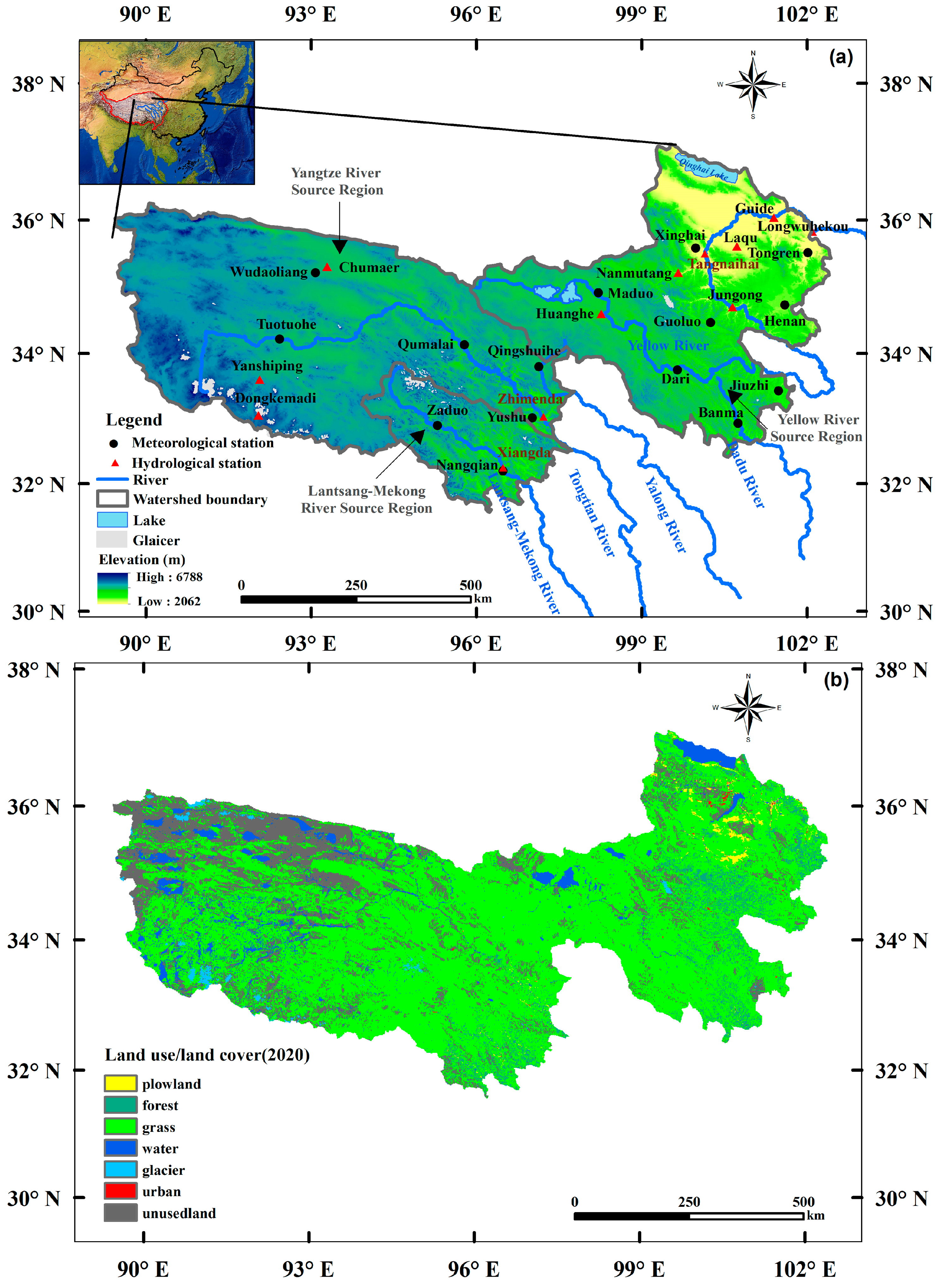
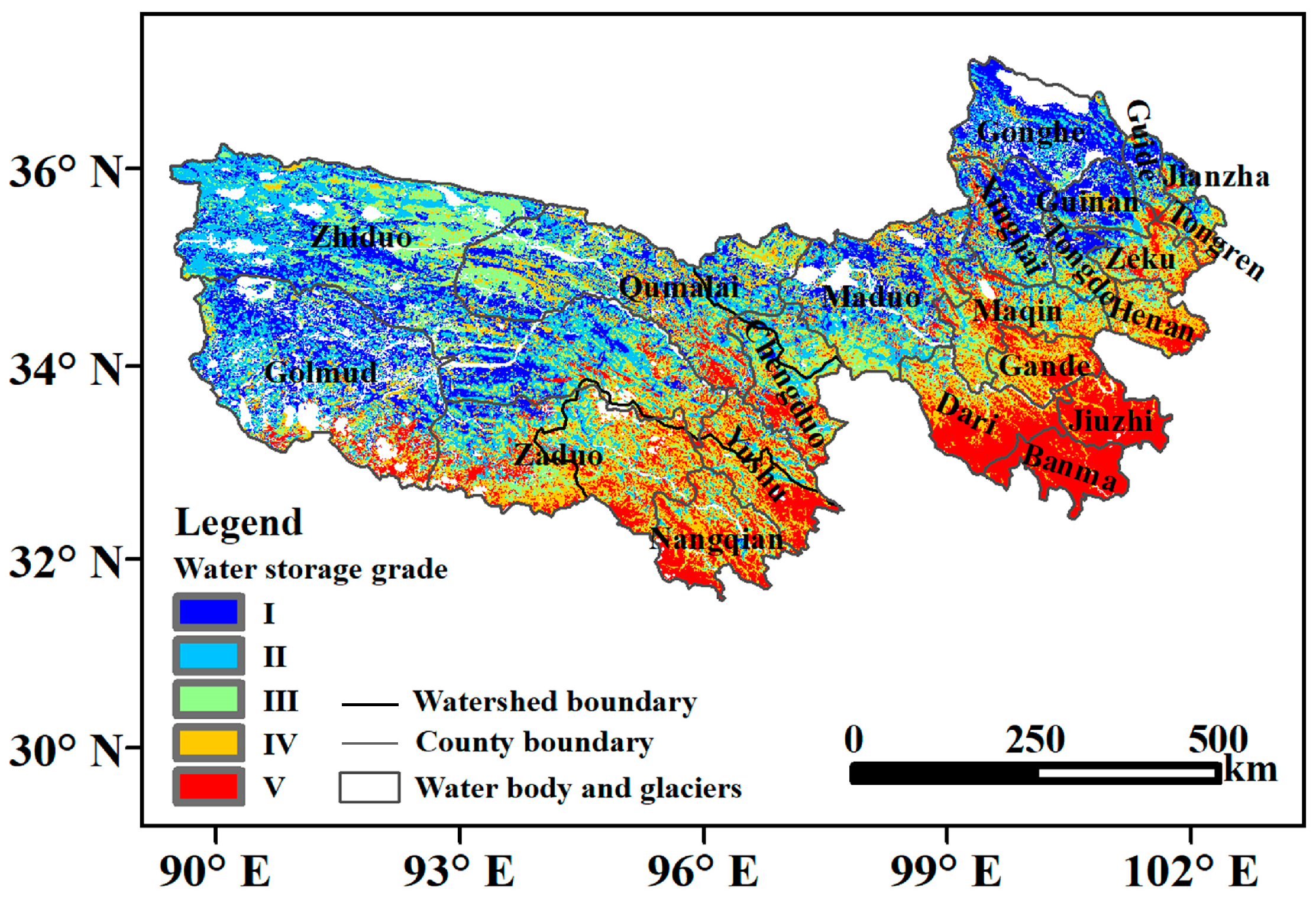
2.1. Study Area

The TRHR (31°39′–36°12′ N, 89°45′–102°23′ E) is the largest National Natural Reserve in China, covering an area of 3.66 × 10⁵ km² on the QTP, which consists of the Yangtze River Headwater region (YAR), the Yellow River Headwater Region (YER), and the Lantsang–Mekong River Headwater Region (LAR) [35] (Figure 1a). The prevailing LULC in the TRHR is predominantly grass, encompassing approximately 71% of the total area, followed by unused land (19%), water body (5%), and forest (4%). Plowland and urban constitute smaller portions of the overall landscape, which are less than 1% (Figure 1b). Encompassing a wide range of elevations, from 2062 m to 6788 m, the study area encompasses extensive expanses of FG [34].

The TRHR is the headwater region of the Yangtze River, the Yellow River, and the Lantsang–Mekong River [34]. The water resources of the TRHR are pivotal to water and food security, economy, and society in the downstream areas, affecting 700 million people downstream [11]. In recent years, there has been a general decline in water resources within the Yellow River Basin, and drought events have been frequent in the Yangtze River Basin, causing extensive economic and ecosystem losses [36,37,38]. Additionally, the severity of water scarcity and flooding of the Yangtze River Basin has been escalating progressively [39]. Owing to the distinctive geographic situation and climate conditions, the TRHR exhibits remarkable fragility, with a harsh natural environment, a modest community structure, and a limited capacity of ecosystems to withstand disturbance and undergo self-repair [40]. Furthermore, the TRHR holds more significant sensitivity to climate change than the global average [41]. In the past few decades, due to the impacts of multiple factors, the water–heat coupling effect on the surface of the TRHR has experienced intricate alterations, resulting in intricate modifications to the WS, further intensifying the uncertainty of the WS [11,31].

2.2. Datasets

From a usage perspective, two types of data were used: model input data and model revision data. The model input data include monthly average Pre, monthly average potential evapotranspiration (ET₀), soil group, LULC, monthly rain event, biophysical table (kc (crop coefficient) and CN (Curve Number)), Digital Elevation Model (DEM), and area of interest (AOI). Model revision data are soil K_sat data and soil Tem data used to correct the soil K_sat of FG and the average monthly air Tem used to consider the effect of SC on WS. The monthly Tem, Pre, and ET₀ were interpolated by Anusplin into 1 km × 1 km raster, and the sources and formats of data, as well as parameters, are shown in

Table 1. Data sources and formats used as inputs of the SWY.

Data Inputs	Format	Source (before Processing into Model Inputs)
Monthly Pre	Raster (1 km)	China Meteorological Data Service Center (http://data.cma.cn) (accessed on 1 January 2021).
Monthly ET0	Raster (1 km)	China Meteorological Data Service Center (http://data.cma.cn) (accessed on 1 January 2021).
Annual LULC	Raster (1 km)	Chinese Academy of Environmental Science Data Center (https://www.resdc.cn/) (accessed on 5 June 2021).
Annual Soil Group	Raster (1 km)	The soil Tem data was downloaded from the National Tibetan Plateau Data Center (http://data.tpdc.ac.cn/) (accessed on 5 November 2020) [42]. Hydrologic Soil Group raster (used as the soil group before revision) and Saturate Hydraulic Conductivity rasters (used to revise the soil group) from FutureWater (https://www.futurewater.eu/2015/07/soil-hydraulic-properties/) (accessed on 4 May 2021).
Biophysical Table)	CSV	CN was downloaded from the United States Department of Agriculture [43]. Kc values were from FAO [44].
Rain Events	CSV	China Meteorological Data Service Center (http://data.cma.cn) (accessed on 1 January 2021).
DEM	Raster (1 km)	Geospatial Data Cloud http://www.gscloud.cn/. (accessed on 5 November 2020)
AOI	Vector	National Tibetan Plateau Data Center (http://data.tpdc.ac.cn/) (accessed on 5 November 2020) [45].
Tf 1	-	−8 °C [46].
T1 1		5 °C [47].
T2 1		2 °C [48].
TFA (Threshold Flow Accumulation) 1	-	3000
α; β; γ 1	-	1/12; 0.4; 1

¹ indicates the model parameters, while the other ones are the inputs of SWY.

. The parameters were set based on the research in the TRHR [34].

2.3. Methods

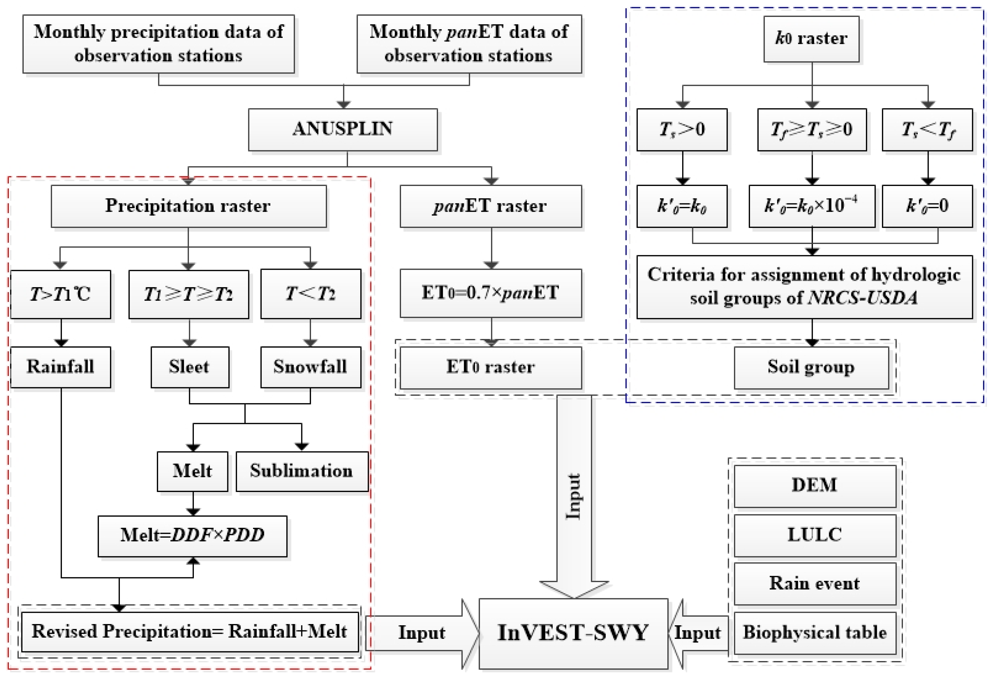
2.3.1. The SWY and Its Revision

The SWY model follows a similar principle to the SWAT model, wherein the monthly quickflow is initially computed using the SCS-CN method [15]:

$$Q{F}_{i,m}=n_m\times \left(\left(a_{i,m}-S_i\right)\exp \left(-\frac{0.2S_i}{a_{i,m}}\right)+\frac{S_i^2}{a_{i,m}}\exp \left(\frac{0.8S_i}{a_{i,m}}\right)E1\left(\frac{S_i}{a_{i,m}}\right)\right)\times \left(25.4\left[\frac{mm}{in}\right]\right)$$

(1)

$$a_{i,m}=\frac{P_{i,m}}{25.4\times n_{i,m}}$$

(2)

$$S_i=\frac{1000}{C{N}_i}-10\left[in\right]$$

(3)

$$E_1\left(x\right)={\displaystyle {\int }_1^{\infty }\frac{e^{-xt}}{t}}dt$$

(4)

where a_i,m represents the monthly average rainfall depth (in), n_i,m denotes rain events, P_i,m signifies the monthly Pre (mm). S_i refers to the maximum potential soil moisture retention capacity after the onset of runoff (inches). CN_i represents the Curve Number. The value 25.4 serves as the conversion factor to convert inches into millimeters (mm).

The annual quickflow (QF_i), is the sum of monthly QF_i,m:

$$Q{F}_i={\displaystyle \sum _{m=1}^{12}Q{F}_{i,m}}$$

(5)

Local recharge (L_i) is obtained by water balance principle:

$$L_i=P_i-Q{F}_i-AE{T}_i$$

(6)

$$AE{T}_{im}=min\left(PE{T}_{i,m};P_{i,m}-Q{F}_{i,m}+{\alpha }_m{\beta }_i{L}_{sum.avail,i}\right)$$

(7)

where P_i represents the annual Pre. L_{sum.avail, i} refers to the summation of subsurface water originating from upgradient sources, which has the potential to be accessible at pixel i:

$$L_{sum.avail,i}={\displaystyle \sum _{j\in \left\{neighbor pixel s draining to pixel i\right\}}{p}_{ij}}·\left(L_{avail,j}+L_{sum.avail,j}\right)$$

(8)

$$L_{avail,i}=min\left(\gamma L_i,L_i\right)$$

(9)

where p_ij ∈ [0, 1] represents the proportion of flow from cell i to j, while L_avail,i refers to the available recharge to a pixel. α_m, β_i, and γ are parameters about topography [34].

In studies that used the SWAT model for modelling WS, the WS is represented by the “L_i”. However, the SWY model incorporates an additional step:

For pixels that are not directly adjacent to the river channel, the cumulative baseflow (B_sum,i) is directly related to the cumulative baseflow discharged by the adjacent downslope pixels:

$$B_{sum,i}=\left\{\begin{array}{cc}{L}_{sum,i}·{\displaystyle \sum _{j\in \left\{\mathrm{cells} \mathrm{to} \mathrm{which} \mathrm{cell} i \mathrm{pours}\right\}}}{p}_{ij}\left(1-\frac{L_{avail.j}}{L_{sum,j}}\right)\frac{B_{sum,j}}{L_{sum,j}-L_i}& \mathrm{if} j \mathrm{is} \mathrm{a} \mathrm{nonstream} \mathrm{pixel}\hfill \\ L_{sum,i}·{\displaystyle \sum _{j\in \left\{\mathrm{cells} \mathrm{to} \mathrm{which} \mathrm{cell} i \mathrm{pours}\right\}}}{p}_{ij}& \mathrm{if} j \mathrm{is} \mathrm{a} \mathrm{stream} \mathrm{pixel}\hfill \end{array}\right.$$

(10)

The cumulative upstream recharge (L_sum,i) is calculated as

$$L_{sum,i}=L_i+{\displaystyle \sum _{j,\mathrm{all} \mathrm{pixels} \mathrm{draining} \mathrm{to} \mathrm{pixel}i}{L}_{sum,j}·p_{ij}}$$

(11)

The baseflow index (B_i) denotes the contribution of a pixel to baseflow. In the case where L_i is negative, B_i is assigned a value of zero. Conversely, B_i is determined by the flow quantity that exits the pixel and the pixel’s relative contribution to the replenishment process:

$$B_i=max\left(B_{sum,i}·\frac{L_i}{L_{sum,i}},0\right)$$

(12)

According to the model principle, B_i is taken as WS. Model inputs of SWY are shown in Table 1 and Figure 2.

The model revision consists of two parts: (1) incorporating the effect of FG on WS by revising its K_sat with soil Tem (Equation (1)), as shown in the blue dashed box of Figure 2; (2) incorporating the effect of snow melt on WS based on the Tem threshold method and the degree-day method (Equations (2) and (3)), as shown in the red dashed box of Figure 2 [34]. Additionally, snow sublimation of the TRHR was estimated according to the study in northeastern Tibetan Plateau (QTP) [49]. The inputs of SWY and flowcharts of incorporating the effects of FG (blue dashed box) and SC (red dashed box) on WS are shown in Figure 2.

$$k{’}_0=\left\{\begin{array}{c}{k}_0\\ k_0\times {10}^{-4}\\ 0\end{array}\right.\begin{array}{cc}& \end{array}\begin{array}{c}{T}_s>0\\ T_f\le T_s\le 0\\ T_s<T_f\end{array}$$

(13)

where k′₀ is the s K_sat (cm/d) after revision. k₀ is the K_sat (cm/d) before revision. T_s is soil Tem. T_f is the Tem threshold of soil freezing.

$$\mathrm{precipitation} \mathrm{types}\left\{\begin{array}{c}\mathrm{rainfall}\\ \mathrm{sleet} \left(\mathrm{mixed}\right)\\ \mathrm{snowfall}\end{array}\right.\begin{array}{cc}& \end{array}\begin{array}{c}{T}_a>T_1\\ T_2\le T_a\le T_1\\ T_a<T_2\end{array}$$

(14)

where T₁ represents the threshold Tem used to distinguish between rain and sleet, T₂ represents the threshold Tem used to differentiate between snow and sleet, and T_a denotes the air Tem.

$$M=DDF·PDD$$

(15)

where M represents the amount of snow melt (mm); DDF refers to the degree-day factor; PDD represents the sum of the average cumulative positive Tem over a specific time period.

2.3.2. Analysis Method

Determination coefficient (R²) was employed to understand the overall correlation between the driving factors and WS (Equation (16)). The correlation is significant when p-value is lower than 0.05.

$$R^2={\left\{\frac{{\displaystyle \sum _{i=1}^n(y_i-\overline{y})(f_i-\overline{f})}}{\sqrt{\frac{1}{n}{\displaystyle \sum _{i=1}^n(y_i-\overline{y}){(f_i-\overline{f})}^2}}}\right\}}^2$$

(16)

where n is the number of time steps, $y_i$ and $f_i$ are the WS and an individual driving factor on the ith time step, respectively, and $\overline{y}$ and $\overline{f}$ are the mean WS and an individual driving factor, respectively.

For the influencing factors of the overall interannual WSC in the TRHR, multiple linear regression analysis was used. In addition, we defined the factor that causes the greatest WSC at each pixel as the predominant influencing factor on WSC at that pixel [50,51]. The steps are as follows:

(1)

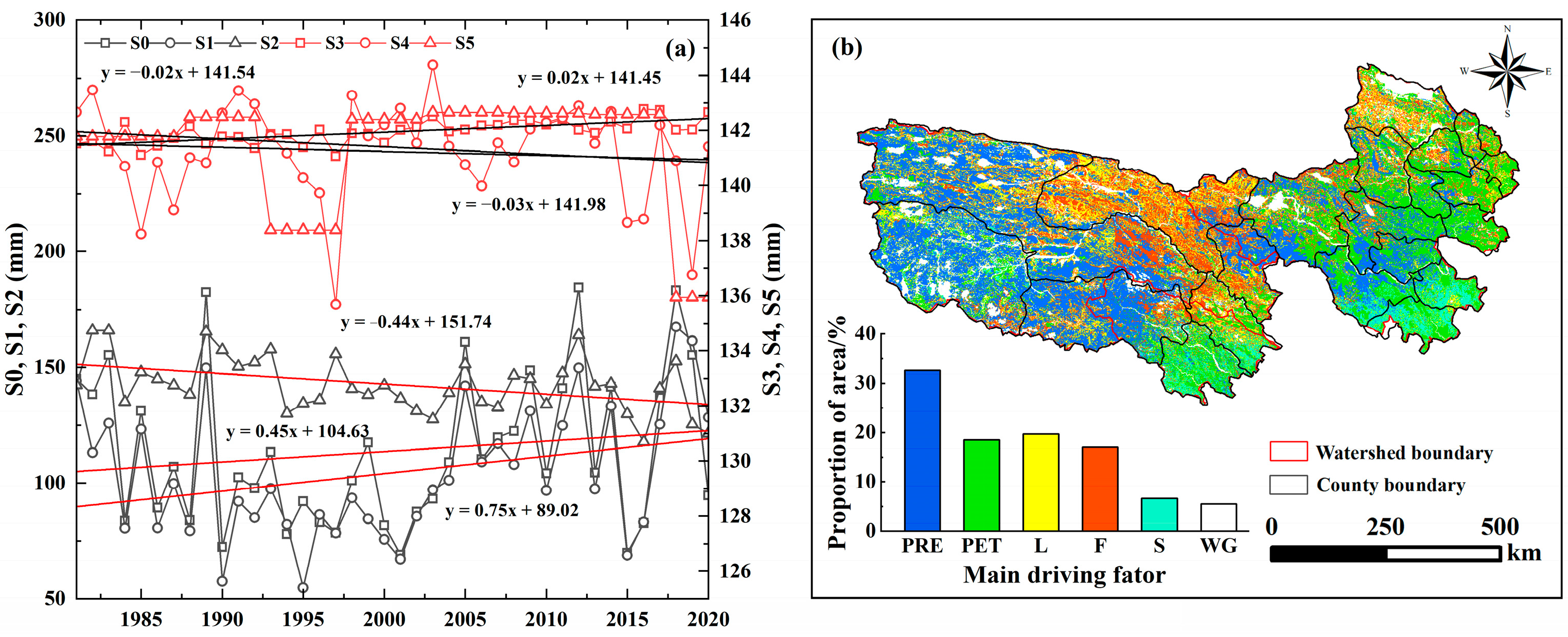
A reference scenario (S0) was established, considering changes in all influencing factors, including Pre, ET₀, LULC, FG, and SC changes. Subsequently, five sensitivity scenarios (sensitivity scenarios A) were created, which are scenarios that consider only changes in Pre (S1), changes in ET₀ (S2), changes in FG (S3), changes in SC (S4), and changes in LULC (S5). By analyzing the trends in WS simulated in S0 and the five sensitivity scenarios, it was possible to understand the effect of each factor on WS. A positive trend signifies a rise in WS, whereas a negative trend indicates a decline in WS. This analysis helps to evaluate the impact of each factor on WS (whether it promotes or inhibits WS).

(2)

Five more sensitivity scenarios (sensitivity scenarios B) were established, where a single influencing factor remains unchanged. These scenarios include only Pre is unchanged (S1′), only ET₀ is unchanged (S2′), only FG is unchanged (S3′), only SC is unchanged (S4′), and only LULC is unchanged (S5′).

Table 2. Model inputs and change trend of modelled WS of each scenario.

Scenarios	Constant Inputs	Inputs for Change from 1981 to 2020	Change Trend of WS (mm/year)
S0	-	Pre, ET0, FG, SC, LULC	0.45
S1	ET0, FG, SC, LULC	Pre	0.75
S2	Pre, ET0, FG, SC, LULC	ET0	−0.44
S3	Pre, ET0, FG, SC, LULC	FG	0.02
S4	Pre, ET0, FG, SC, LULC	SC	−0.03
S5	Pre, ET0, FG, SC, LULC	LULC	−0.02
S1′	Pre	ET0, FG, SC, LULC	-
S2′	ET0	Pre, FG, SC, LULC	-
S3′	FG	Pre, ET0, SC, LULC	-
S4′	SC	Pre, ET0, FG, LULC	-
S5′	LULC	Pre, ET0, FG, SC	-

shows the model inputs for each scenario.

(3)

To obtain the contribution of each factor to WSC, the absolute value of the difference between the WS modelled by S0 and the five scenarios of sensitivity scenario B was calculated. The largest one of absolute values of the contribution was taken as the dominant factor influencing the WSC at that pixel.

2.3.3. Trend Analysis Method

Trends in WS, annual average Tem, annual Pre, and annual ET₀ from 1981 to 2020 were examined through linear regression analysis (Equation (17)). Spatial trend analysis is conducted for individual pixels to investigate any changes in trends.

$$Slope=\frac{n{\displaystyle \sum _{i=1}^n(i{V}_i)-{\displaystyle \sum _{i-1}^{n}i{\displaystyle \sum _{i-1}^n{V}_i}}}}{n{\displaystyle \sum _{i=1}^n{i}^2-({\displaystyle \sum _{i=1}^{n}i{)}^2}}}$$

(17)

where n represents the number of years (n = 40 here), i ranges from 1 to n, and V_i signifies the value of the variable in year i. If the slope (Slope) is greater than 0, it indicates an increasing trend in the variable throughout the study period. Conversely, if the slope is less than 0, it signifies decreasing trend. The p value is used as the criterion for significant test with a significance threshold of 0.05.

2.3.4. Method for Spatial Division of WS Importance

The importance of WS in the TRHR was classfied by the quantile classification method in ArcGIS based on the Technical Guidelines for the Delineation of Red Line for Ecological Protection developed by [18].

3. Results

3.1. Spatiotemporal Variation in Water Storage

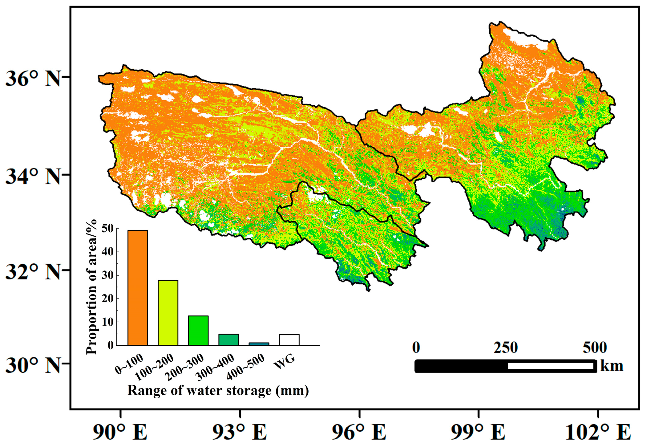
3.1.1. Spatial Distribution of Annual Water Storage

The increase in WS occurs from northwest to southeast according to the pattern of Pre (Figure 3 and Figure 4b). The WS ranges from 0 to 500 mm, and the area occupied by each range decreases as the WS increases. The majority of the WS falls within the range of 0–100 mm, accounting for 49.10% of the region. This range is predominantly distributed in the eastern and northern YAR and YER. The range of 100–200 mm represents 27.70% of the TRHR and is distributed in the northeastern, southeastern, and southern YAR, as well as in the eastern and central–southern YER. The range of 200–300 mm accounts for 12.30% of the total area and is mainly distributed in the eastern and southern parts of the YAR and YER, as well as in the southeast of the LAR. The range of 300–400 mm occupies only 4.6% of the TRHR, which is mainly distributed in the southwestern YER and southwestern LAR.

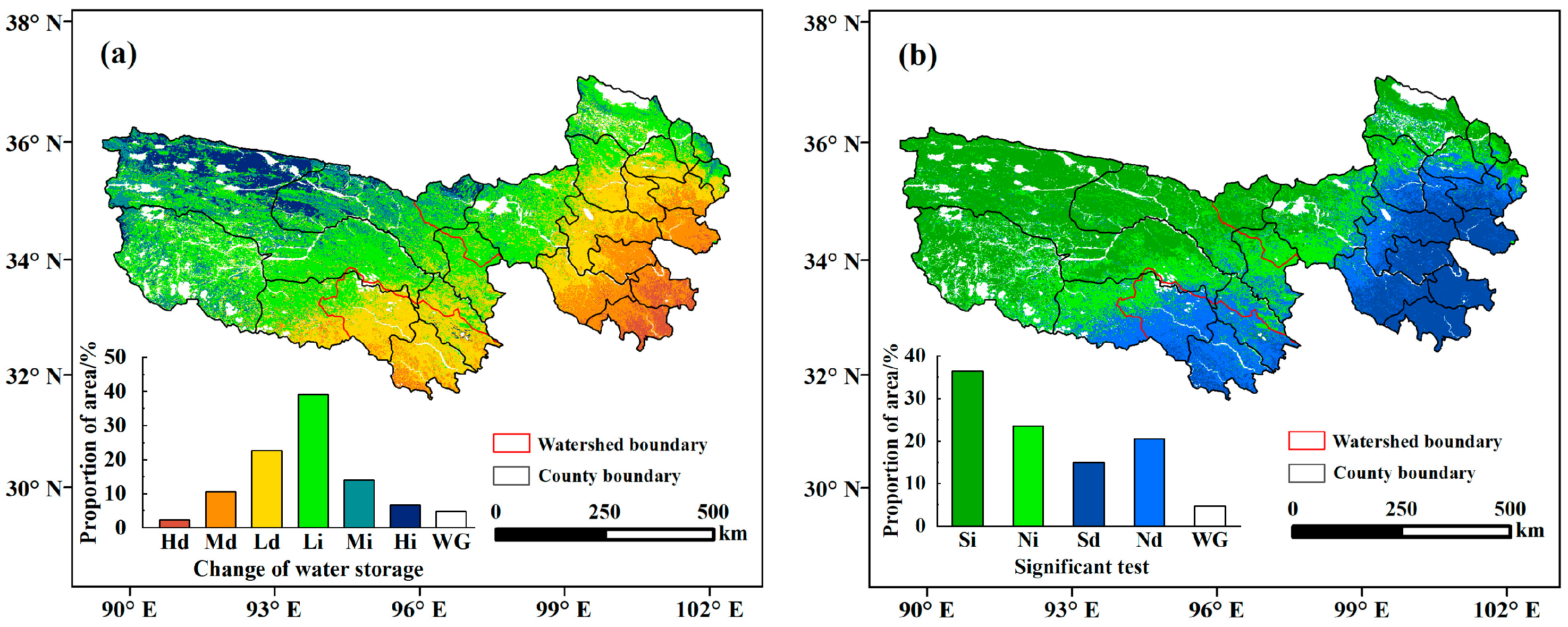
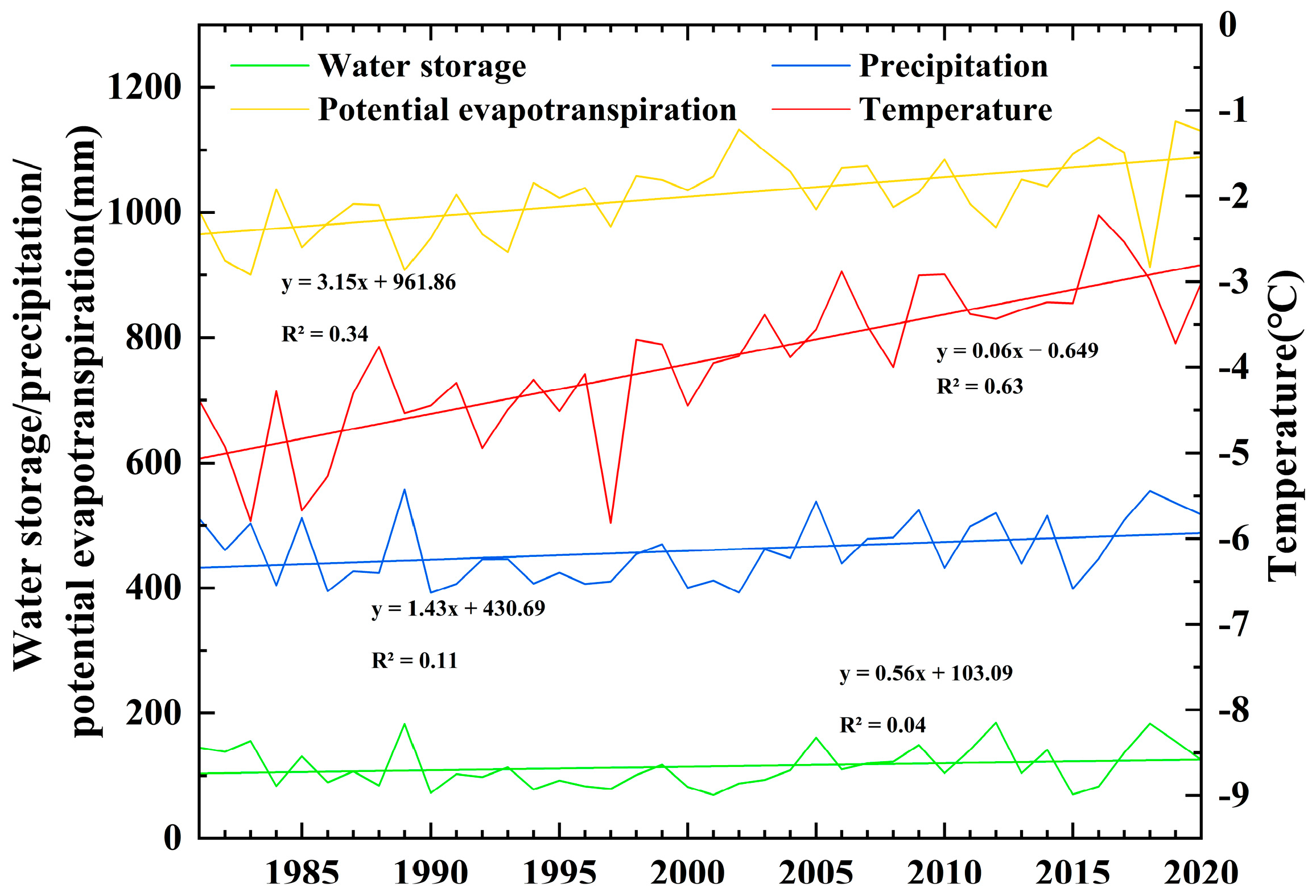
3.1.2. Change in Annual Average Water Storage

The WS exhibited an upward trend in fluctuation from 1981 to 2020, at a rate of 0.56 mm/year (Figure 5). The muti-year average WS within the TRHR was 35.46 mm, constituting 24.93% of the annual Pre. The maximum WS occurred in 2012 (184.49 mm), while the minimum occurred in 2001 (69.03 mm).

Although the overall WS in the TRHR increased from 1981 to 2020, the spatial changes varied from northwest to southeast, with a significant upward trend, a non-significant upward trend, a non-significant downward trend, and a significant downward trend in that order (Figure 6b). The area exhibiting a positive trend in WS amounted to 60.04%, whereas the portion displaying a negative trend accounted for 34.76%. Among the areas with significant changes, 51.19% of the total area showed significant trends, with 36.39% significantly increasing and 14.80% significantly decreasing. The areas with no significant changes in WS accounted for 43.61%, of which 23.44% exhibited non-significant increasing trends and 20.17% displayed non-significant decreasing trends. The regions demonstrating increasing trends in WS were predominantly found in the YAR, as well as the western and northern YER, with a small portion in the northwestern LAR. The rate of increase varied between 0 and 7 mm/year, and the area experiencing high-speed increase (4–7 mm/year) accounted for 6.66% of the TRHR, primarily located in the northern YAR (Figure 6a). The area of medium-speed increase (2–4 mm/year) accounted for 14.05% and was distributed in the northwestern TRHR. The low-speed increasing (0–2 mm/year) region accounted for 39.12% and was located in the southeastern YAR and western and northern YER. Both the areas of high-speed and medium-speed increase all passed the significance test. The regions exhibiting a decreasing trend were located in the LAR and central and northwestern YER. The decreasing rate range is −10–0 mm/year. The areas with high-speed decrease (−10–6 mm/year) accounted for 2.30% of the TRHR and were primarily located within a small portion of the southeastern YER. The areas with medium-speed decrease (−6–−3 mm/year) accounted for 10.54% of the TRHR and were located in the southeastern YER and southern LAR. The regions with low-speed decrease (−3–0 mm/year) accounted for 22.61% and were located in the central YER and most of the LAR. Both the locations of high-speed and medium-speed decrease were significant decrease areas.

3.2. Main Driving Factors of Water Storage

Figure 5 illustrates the annual average air Tem, annual Pre, annual ET₀, and annual WS of the TRHR during 1981–2020. The annual mean air Tem showed an upward trend in the last 40 years (0.05 °C/year). The mean multi-year Tem was 0.25 °C, with the highest Tem recorded in 2016 (1.42 °C) and the lowest Tem recorded in 1983 (−1.22 °C). The average annual Pre was 459.91 mm, with an increasing rate of 1.43 mm/year. The highest annual Pre was observed in 1989 (557.26 mm), whereas the lowest was observed in 2002 (392.66 mm). The average ET₀ was 1026.53 mm, exhibiting an upward trend of 3.15 mm/year. The peak ET₀ value was in 2002 (1132.79 mm), while the lowest value was in 1983 (900.62 mm). Based on a multiple linear regression analysis, the overall WS in the TRHR from 1981 to 2020 was found to be most influenced by Pre (R² = 0.81, p < 0.05). ET₀ also had an influence (R² = 0.32, p < 0.05), but air Tem did not show a significant effect (R² = 0.02, p > 0.05).

The trends in WS simulated by S0, S1, S2, S3, S4, and S5 from 1981 to 2020 are shown in Figure 7a. The trend of S1 is generally similar to that of S0. Both scenarios show an upward trend (4.5 mm/10 year and 7.5 mm/10 year, respectively), indicating that Pre promotes WS. S2 shows a decrease at a rate of 4.4 mm/10 year, indicating that ET₀ inhibits WS. In comparison to S1 and S2, the changes observed in S3, S4, and S5 are relatively minor. S3 demonstrates a marginal increase with a rate of 0.2 mm/10 year, while S4 and S5 display decreasing trends (−0.3 mm/10 year and −0.2 mm/10 year). This suggests that change in permeability of FG contributes to changes in WS, while SC and LULC inhibit WS. However, the effects of these factors are relatively small compared to Pre and ET₀ in. When the rate of WSC for each sensitivity scenario is combined, it still does not reach the level of the S0. This indicates that the WS in the TRHR is also affected by other human activities. These additional influences result in an increase in WS at a rate of 2.8 mm/10 years.

The analysis of the dominant influencing factors on WSC in each pixel provides more detailed insights into the underlying causes of the changes in WS in different locations within the TRHR (Figure 7b). Further, 32.62% of the TRHR is primarily influenced by Pre, which is predominantly concentrated in the LAR and northwestern YAR, with less distribution in the YER. The trend of Pre changes in these areas is consistent with that of the WS. In other words, an upward (or downward) trend in Pre leads to an upward (or downward) trend in WS (Figure 4e and Figure 6).

The area mainly influenced by LULC accounted for 19.69% of the TRHR and is not concentrated in a specific region, which was directly related to changes in LULC patterns. The distribution of areas with changes in LULC in the TRHR was more sporadic during the periods of 1980–1990, 1990–1995, 1995–2000, and 2015–2020. However, the LULC values were almost unchanged during the periods of 2000–2005, 2005–2010, and 2010–2015 (Figure 8). In general, areas changed from unused land to grass, which accounted for 30.65% of the TRHR. This was followed by the conversion of grass into unused land, which accounted for 26.54% of the TRHR. The conversion between grass and forest remained relatively stable, at 8.32% and 8.40%, respectively, while the other land use types had relatively minor changes (

Table 3. LULC changes in the TRHR as a percentage of the TRHR and the resulting changes in unit WS.

	1980–1990		1990–1995		1995–2000		2015–2020
	LULC Change (%)	Unit WSC (mm)	LULC Change (%)	Unit WSC (mm)	LULC Change (%)	Unit WSC (mm)	LULC Change (%)	Unit WSC (mm)
grass to unused land	6.47	162.58	6.28	161.08	8.86	154.22	4.93	144.46
unused land to grass	6.47	−160.97	9.50	−156.34	5.52	−160.47	9.16	−161.25
grass to forest	2.20	63.64	1.90	64.51	2.00	62.05	2.21	64.75
forest to grass	2.19	−63.69	2.30	−62.99	1.62	−63.30	2.29	−63.27
forest to unused land	0.12	137.29	0.10	147.49	0.07	134.86	0.07	129.57
unused land to forest	0.10	−133.80	0.09	−130.96	0.12	−152.25	0.11	−133.28
grass to plowland	0.21	−12.58	0.21	−9.65	0.14	−13.61	0.23	−9.37
plowland to grass	0.17	12.19	0.16	16.28	0.17	11.22	0.21	14.57

). The unit WS increased by 155.6 mm in the areas converted from grass to unused land, while it decreased by 159.8 mm in the areas converted from unused land to grass. The unit WS in the areas converted from grass to forest increased by 63.7 mm, while it decreased by 63.3 mm in the areas converted from forest to grass. Additionally, the unit WS in the areas converted from forest to unused land increased by 13.3 mm, while it decreased by 137.6 mm in the areas converted from unused land to forest. The areas converted from grass to plowland decreased by 11.3 mm in terms of unit WS but increased by 13.5 mm in the areas converted from plowland to grass. These findings indicate that areas without vegetation cover have a higher WS capacity compared to areas with vegetation cover. For areas covered by vegetation, the WS capacity follows a descending order: forest, grass, and plowland. This may be attributed to increased AET due to increased vegetation cover, which reduces the available water quantity.

The region primarily impacted by ET₀ comprises 18.49% of the TRHR. It is predominantly situated in the southeast of the YER and LAR, where ET₀ experiences significant increases at a high rate, and WS shows a decreasing trend (Figure 4f and Figure 6). It shows that augmentation of ET₀ results in a decline in WS. The area mainly affected by fFG accounts for 17.05% of the TRHR. It is predominantly found in the eastern YAR and northern YER. These areas exhibit an overall rising Tem trend (Figure 4d), with the YAR experiencing a more pronounced rate of warming. Conversely, the northern YER, which is mainly affected by FG, shows a comparatively slower rate of warming. Nonetheless, the air Tem remains relatively high, ranging from 0 to 9 °C (Figure 4a). Warmer temperatures will increase the hydraulic conductivity of the soil [52], increase water infiltration, and thus increase WS.

The region primarily impacted by SC constituted 6.64% of the TRHR. Within the LAR, the areas influenced by SC exhibited temperatures ranging from −4 to 0 °C, whereas, in the YER, the temperatures ranged from −6 to 0 °C. Consequently, snowfall was the primary form of Pre in these areas [47,48]. The sublimation process outweighed the ablation process, resulting in a reduction in WS.

3.3. Spatial Division of Water Storage Importance

The important classifications for the five levels of WS were established: <29 mm for grade I, 29–75 mm for grade II, 75–127 mm for grade III, 127–206 mm for grade IV, and >206 mm for grade V (Figure 9).

Class V are predominantly located in the eastern and southern YAR, southern YER, and eastern and southern LAR (counties: southern Golmud, Zaduo, southeastern Yushu, Nangqian, southern Chengduo, southern Qumalai, southern Maqin, southern Henan, Gande, southern Dari, Jiuzhi, and Banma). Most of these areas exhibit a significantly high rate of decline in WS (Figure 6). Class IV are primarily distributed in the eastern and southern YAR, southern and central YER, and southeastern LAR (counties: Golmud, Zaduo, Nangqian, Yushu, northern Qumailai, northern Dari, Gande, Maqin, Henan, Zeku, and Tongren). Similarly, these areas experience decreasing trends in WS (Figure 9). Class III are mainly situated in the northeastern and southern YAR, the central–southern YER, and central LAR (counties: northern Zhiduo, eastern and western Qumalai, Zaduo, northern Nangqian, Yushu, northern Chengduo, southern Maduo, northern Dari, western Gande, Maqin, Henan, and Zeku). With the exception of Qumalai and Maduo, the remaining areas generally display decreasing trends. Class II are primarily found in the western and central–southern YAR, as well as western YER (counties: western Golmud, Zhiduo, Qumalai, Maduo, and northern Zaduo), with a greater number of WS showing an increasing trend. Class I is mainly distributed in the YAR and western and northern YER (counties: Golmud, Zhiduo, northern Qumalai, northern Xinghai, Gonghe, Guinan, Guide, northern Jianzha, and northern Tongde). The WS capacity in these regions demonstrates a significant increasing trend. In general, the YAR is predominantly classified as Level I, II, and III, while the YER increased from Level I to Level V from north to south, and the LAR is mainly categorized as Level IV and V.

4. Discussion

4.1. Main Driving Factors of Water Storage

Previous studies have consistently demonstrated that WS increases with Pre and decreases with ET₀ [9,18,23]. However, WS is impacted by a confluence of factors, and the primary factors vary across different regions. Xu et al., found that Pre is the most prominent factor influencing WS in the Qilian Mountains [9]. Bai et al. found that climate change yields more substantial influence on WS than LULC in Kentucky, USA [53]. Wang et al.’s study showed that other human activities were the primary factor contributing to the decline in WS from 1960 to 2016, with climate change as a secondary factor [31]. While these studies have provided insights into the contributions of various factors to the study areas, they have not explored the primary driving factors in each specific region spatially.

There have been several research studies about the spatiotemporal changes and influence factors of WS in the TRHR. The research conducted by Xue et al. indicated that, from 1981 to 2019, TRHR’s WS exhibited an upward trend. This notable trend was accompanied by a regional distribution that increased progressively from northwest to southeast. Moreover, the findings indicated that heightened levels of Pre would contribute to an augmentation in WS [30]. The outcomes of our study align with previous research conducted in the Three-River Headwaters National Park and the QTP [31,54]. Nevertheless, the findings of this work differ from previous studies in several aspects. Firstly, none of the aforementioned studies took into account the effects of FG and SC on WS. When analyzing the factors affecting WS, they primarily focused on climate elements, LULC, and topographic characteristics. However, the significance of SC, as a key influencing factor for WS in Class V and Class IV, cannot be disregarded. With the ongoing climate warming, the effect of FG on WS cannot be ignored. Zhao et al. demonstrated that neglecting the effect of SC would result in an overestimation of the average annual WS in TRHR by 13 mm/year). Similarly, disregarding the effect of FG would lead to an average overestimation of WS by 6 mm/year) [34]. SC change decreased WS at a rate of 0.3 mm/10 yr, while FG change increased WS at a rate of 0.2 mm/10 year. Although the latter occurs at a slower rate, it should not be disregarded over larger areas and over longer time scales. Furthermore, Wang et al.’s study concluded that an increase in NDVI (Normalized Difference Vegetation Index) leads to an increment in WS [31]. Xue et al. found that the unit WS of each LULC of the TRHR is forest, grass, plowland, and other types in descending order [30]. In this research, the ranking order of WS remained the same for forest, grass, and plowland, except that converting grass or forest into unused land increased the WS capacity. Unused land mainly refers to areas with less than 5% vegetation cover, while grass encompasses areas with 5–50% vegetation cover. The results of previous studies mentioned above indicate that an increase in vegetation cover results in an augmentation of WS, whereas the findings of this paper demonstrate the opposite. Numerous studies have provided evidence that vegetation greening has the effect of reducing water yield through the promotion of AET. In the study by Bai et al., it was revealed that vegetation greening resulted in an elevation of AET and a concurrent reduction in water yield in China during 1982–2014 [55]. Additionally, it was estimated that the grass wetland and forest of the QTP would experience an increase of 1.04%, 6.01%, and 0.07%, respectively, from 2010 to 2030 [54]. However, this expansion in vegetation is expected to result in a slight decrease in water yield by 0.007% [56]. Research conducted in the Yangtze River Basin has demonstrated that climate change masks the impacts of vegetation greening on water quantity, and that land “greening” accelerates the regional hydrological cycle through increased AET, resulting in an augmented risk of water scarcity [33]. Similarly, Liu et al., revealed that increased vegetation of the Yellow River led to a substantial increase in AET, consequently decreasing water yield [57].

4.2. Implications for Water Management

Currently, the research on the factors influencing WS primarily focuses on analyzing the overall factors affecting regional WS without specifically examining the main reasons for WSC in different parts of the region. Meanwhile, these studies often overlook the influence of cryosphere elements on WS. Using the revised SWY that considered the effects of FG and SC on WS, this study analyzed the principal influencing factors of WSC at a 1 km grid scale in each pixel of the TRHR. It provides detailed maps illustrating the main factors influencing WSC in various locations within the region. This analysis can offer more useful information for decisionmakers.

The southwestern part of Nangqian County, southeastern part of Yushu County, and southern parts of Dari County, Jiuzhi County, and Banma County are classified as extremely and highly important regarding WS, and it is crucial to protect these areas. However, these regions are experiencing a notable decline in WS, mainly due to snow sublimation and increased ET₀. Previous studies have indicated that humid climate conditions can inhibit snow and ice sublimation [58,59,60,61]. The effect of increased vegetation on water quantity has been a subject of debate. As mentioned in Section 4.1, most evidence suggests that increased vegetation leads to higher AET, resulting in reduced water yield [62,63,64]. Nonetheless, there is still some evidence suggesting that vegetation changes have minimal effects or may even increase water yield, particularly in areas with humid climates [65,66]. It is worth noting that vegetation plays a critical role in ecosystems by preventing soil erosion, storing carbon, regulating water resources, controlling climate, and connecting the hydrosphere, biosphere, and atmosphere [67,68]. This study concludes that converting unused land with 5% vegetation cover to grass and forest with higher vegetation cover reduces water yield by increasing AET. Therefore, it is inappropriate to adopt an approach of decreasing vegetation cover to reduce the increase in AET caused by greening effects. Some researchers have proposed strategies such as allowing natural regeneration of native vegetation and avoiding the use of fast-growing non-native vegetation species in vegetation restoration and greening to minimize water consumption while achieving soil erosion control and ecological restoration [66,67,68]. It is noteworthy that, while the greening of vegetation enhances AET, the land–atmosphere system is a fully interconnected system. Focusing solely on the rise in AET attributed to vegetation restoration as a separate factor influencing the observed climatic elements would amplify the adverse impacts of vegetation restoration on surface water availability [69]. The increase in WS can be attributed to the increase in Pre exceeding the increase in AET. Over the long term, the amplification of Pre caused by the greening of vegetation, influenced by atmospheric circulation, in turn, supports and enhances WS. This crucial feedback process is frequently disregarded. Henceforth, in the analysis of the effect of vegetation on WS, it is imperative to acknowledge the feedback of vegetation to Pre. From a perspective of long-term sustainability, the greening of vegetation will foster favorable conditions for WS.

4.3. Limitations of This Study

Firstly, although the InVEST model, as the most popular ecosystem service model, possesses a relatively simple structure and is user-friendly, it lacks the complexity of traditional hydrological models. The SWY employed in this study does not encompass intricate hydrophysical processes, which introduces uncertainties into the model outputs. Secondly, the model fails to explicitly incorporate the effect of human activities on WS, which are mainly grazing in the TRHR [70]. Thirdly, the current model used here accounts for the effects of cryosphere elements on WS, excluding glaciers. However, there are 1238 glaciers in the TRHR, covering approximately 1218 km² with a total glacier volume of around 87.66 km³. Although this comprises a relatively minute fraction of the TRHR (0.33%) [71], it is crucial to consider this aspect from a more accurate perspective. Fourthly, the incorporated frozen module in this model primarily focuses on the effect of changes in FG permeability on WS. However, the hydrological processes of the FG are complex, such as the contribution of ablation to runoff and the increased water storage capacity resulting from the thickening of the active layer, which should be considered comprehensively [72,73]. Finally, given that the input data of SWY consist of ET₀ data, rather than AET data, the ET₀ data are employed in the examination of the factors influencing WSC through sensitivity analysis. The means of improvement in a future study could be as follows: integrating glacier melt into models, analyzing FG and AET on WS utilizing remote sensing data, and taking into account the repercussions of grazing on WS in the TRHR by fieldwork and sampling.

5. Conclusions

This study analyzes the spatiotemporal changes and driving factors regarding WSC in the TRHR, employing a revised SWY that takes the effects of FG and SC on WS into account. The conclusions are as follows:

From 1981 to 2020, the TRHR experienced an overall increase in WS, which generally exhibited a spatial pattern increasing from northwest to southeast. The spatial changes within the area showed a significant increasing trend, followed by a non-significant increasing trend, a non-significant decreasing trend, and a significant decreasing trend from northwest to southeast, in that order, with respective proportions of 36.39%, 23.44%, 20.17%, and 14.80%. The increasing Pre resulted in an increase in WS. Conversely, the intensification of ET₀ led to a reduction in WS. Climate-induced FG degradation enhanced soil permeability, thereby increasing WS, while both SC and LULC changes resulted in a decline in WS.

This study identified the Pre-affected region as the most expansive, encompassing a substantial portion of the study area, amounting to 32.62% of the TRHR, followed by LULC (19.69%), ET₀ (18.49%), FG (17.05%), and SC (6.64%). Based on the spatial division of WS importance, eastern and southern YAR, southern YER, and eastern and southern LAR (counties: southern Golmud, Zaduo, southeastern Yushu, Nangqian, southern Chengduo, southern Qumalai, southern Maqin, southern Henan, Gande, southern Dari, Jiuzhi, and Banma) were classified as extremely important and highly important WS zones. These regions exhibit a decreasing trend in WS and necessitate the attention of policymakers, who should implement appropriate measures to protect and enhance their ecological conditions.

Although this study provides valuable insights, it is important to acknowledge certain limitations. Firstly, uncertainties associated with the model itself should be acknowledged. Furthermore, the effect of human activities and glaciers on WS was not explicitly taken into account, which could have influenced the results. Additionally, the description of FG hydrological processes may not have been comprehensive enough, highlighting the need for future model improvements in this regard. Addressing these limitations and enhancing the understanding of these factors will be a key focus of our future research endeavors.

References

- Vörösmarty, C.J.; Hoekstra, A.Y.; Bunn, S.E.; Conway, D.; Gupta, J. Fresh water goes global. Science 2015, 349, 478–479. [Google Scholar] [CrossRef] [PubMed]
- Palmer, M.; Ruhi, A. Linkages between flow regime, biota, and ecosystem processes: Implications for river restoration. Science 2019, 365, eaaw2087. [Google Scholar] [CrossRef] [PubMed]
- Benra, F.; Frutos, A.; Gaglio, M.; Alvarez-Garreton, C.; Feilipe-Lucia, M. Mapping water ecosystem services: Evaluating InVEST model predictions in data scarce regions. Environ. Model. Softw. 2021, 138, 104982. [Google Scholar] [CrossRef]
- Abdelhaleem, F.S.; Basiouny, M.; Ashour, E.; Mahmoud, A. Application of remote sensing and geographic information systems in irrigation water management under water scarcity conditions in Fayoum, Egypt. J. Environ. Manag. 2021, 299, 113683. [Google Scholar] [CrossRef]
- Lv, Y.; Hu, J.; Sun, F.; Zhang, L. Water retention and hydrological regulation: Harmony but not the same in terrestrial hydrological ecosystem services. Acta Ecol. Sin. 2015, 35, 5191–5196. (In Chinese) [Google Scholar]
- Wang, Y.; Ye, A.; Qiao, F.; Li, Z.; Miao, C.; Di, Z.; Gong, W. Review on connotation and estimation method of water conservation. South-North Water Transf. Water Sci. Technol. 2021, 19, 10451–11071. (In Chinese) [Google Scholar]
- Wang, S.; Zhang, B.; Wang, S. Dynamic changes in water conservation in the Beijing–Tianjin sandstorm source control project area: A case study of Xilin Gol League in China. J. Clean. Prod. 2021, 293, 126054. [Google Scholar] [CrossRef]
- Chen, J.; Wang, D.; Li, G.; Sun, Z.; Wang, X.; Zhang, X.; Zhang, W. Spatial and temporal heterogeneity analysis of water conservation in Beijing-Tianjin-Hebei urban agglomeration based on the geodetector and spatial elastic coefficient trajectory models. GeoHealth 2020, 4, e2020GH000248. [Google Scholar] [CrossRef]
- Xu, H.; Zhao, C.; Wang, X.; Chen, S.; Shan, S.; Chen, T.; Qi, X. Spatial differentiation of determinants for water conservation dynamics in a dryland mountain. J. Clean. Prod. 2022, 362, 132574. [Google Scholar] [CrossRef]
- Kittredge, J. Forest Influences: The Effects of Woody Vegetation on Climate, Water, and Soil, with Applications to the Conservation of Water and the Control of Floods and Erosion; Mc Graw-Hill Book Co., Inc.: New York, NY, USA, 1948. [Google Scholar]
- Deng, M.; Shi, P.; Xie, G. Water Conservation of Forest Ecosystem in the Upper Reaches of the Yangtze River and Its Benefits. Resour. Sci. 2002, 24, 68–73. (In Chinese) [Google Scholar]
- Zhang, B.; Li, W.; Xie, G.; Xiao, Y. Water conservation function and measurement methods of forest ecosystems. Chin. J. Ecol. 2009, 28, 529–534. (In Chinese) [Google Scholar]
- Gong, S.; Xiao, Y.; Zheng, H.; Xiao, Y.; Ouyang, Z. Spatial patterns of ecosystem water conservation in China and its impact factors analysis. Acta Ecol. Sin. 2017, 37, 2455–2462. (In Chinese) [Google Scholar]
- Cao, W.; Wu, D.; Huang, L.; Liu, L. Spatial and temporal variations and significance identification of ecosystem services in the Sanjiangyuan National Park, China. Sci. Rep. 2020, 10, 6151. [Google Scholar] [CrossRef] [PubMed]
- Sharp, R.; Douglass, J.; Wolny, S.; Arkema, K.; Bernhardt, J.; Bierbower, W.; Chaumont, N.; Denu, D.; Fisher, D.; Glowinski, K.; et al. InVEST 3.9.0. User’s Guide—The Natural Capital Project; Stanford University: Stanford, CA, USA, 2020. [Google Scholar]
- Hu, W.; Li, G.; Li, Z. Spatial and temporal evolution characteristics of the water conservation function and its driving factors in regional lake wetlands—Two types of homogeneous lakes as examples. Ecol. Indic. 2021, 130, 108069. [Google Scholar] [CrossRef]
- Jia, G.; Hu, W.; Zhang, B.; Li, G.; Shen, S.; Gao, Z.; Li, Y. Assessing impacts of the Ecological Retreat project on water conservation in the Yellow River Basin. Sci. Total Environ. 2022, 828, 154483. [Google Scholar] [CrossRef]
- Li, M.; Liang, D.; Xia, J.; Song, J.; Cheng, D.; Wu, J.; Li, Q. Evaluation of water conservation function of Danjiang River Basin in Qinling Mountains, China based on InVEST model. J. Environ. Manag. 2021, 286, 112212. [Google Scholar] [CrossRef]
- Huang, X.; Liu, J.; Peng, S.; Huang, B. The impact of multi-scenario land use change on the water conservation in central Yunnan urban agglomeration, China. Ecol. Indic. 2023, 147, 109922. [Google Scholar] [CrossRef]
- Qin, H.; Chen, Y. Spatial non-stationarity of water conservation services and landscape patterns in Erhai Lake Basin, China. Ecol. Indic. 2023, 146, 109894. [Google Scholar] [CrossRef]
- Vigerstol, K.; Aukema, J. A comparison of tools for modeling freshwater ecosystem services. J. Environ. Manag. 2010, 92, 2403–2409. [Google Scholar] [CrossRef]
- Zuo, D.; Chen, G.; Wang, G.; Xu, Z.; Han, Y.; Peng, D.; Pang, B.; Abbaspour, A.; Yang, H. Assessment of changes in water conservation capacity under land degradation neutrality effects in a typical watershed of Yellow River Basin, China. Ecol. Indic. 2023, 148, 110145. [Google Scholar] [CrossRef]
- Wu, Q.; Song, J.; Sun, H.; Huang, P.; Jing, K.; Xu, W.; Wang, H.; Liang, D. Spatiotemporal variations of water conservation function based on EOF analysis at multi time scales under different ecosystems of Heihe River Basin. J. Environ. Manag. 2023, 325, 116532. [Google Scholar] [CrossRef] [PubMed]
- Zhang, G.; Wu, Y.; Li, H.; Zhao, W.; Wang, F.; Chen, J.; Sivakumar, B.; Liu, S.; Qiu, L.; Wang, W. Assessment of water retention variation and risk warning under climate change in an inner headwater basin in the 21st century. J. Hydrol. 2022, 615, 128717. [Google Scholar] [CrossRef]
- Bai, Y.; Guo, C.; Degen, A.A.; Ahmad, A.A.; Wang, W.; Zhang, T.; Shang, Z. Climate warming benefits alpine vegetation growth in Three-River Headwater Region, China. Sci. Total Environ. 2020, 742, 140574. [Google Scholar] [CrossRef] [PubMed]
- Wang, J.; Zhou, W.; Guan, Y. Optimization of management by analyzing ecosystem service value variations in different watersheds in the Three-River Headwaters Basin. J. Environ. Manag. 2022, 321, 115956. [Google Scholar] [CrossRef] [PubMed]
- Wang, T.; Yang, D.; Qin, Y.; Wang, Y.; Chen, Y.; Gao, B.; Yang, H. Historical and future changes of frozen ground in the upper Yellow River Basin. Glob. Planet. Chang. 2018, 162, 199–211. [Google Scholar] [CrossRef]
- Wang, Y.; Yang, H.; Gao, B.; Wang, T.; Qin, Y.; Yang, D. Frozen ground degradation may reduce future runoff in the headwaters of an inland river on the northeastern Tibetan Plateau. J. Hydrol. 2018, 564, S0022169418305924. [Google Scholar] [CrossRef]
- Pan, T.; Wu, S.; Dai, E.; Liu, S. Spatiotemporal variation of water source supply service in Three Rivers Source Area of China based on InVEST model. J Appl Ecol. 2013, 24, 183–189. (In Chinese) [Google Scholar]
- Xue, J.; Li, Z.; Feng, Q.; Gui, J.; Zhang, B. Spatiotemporal variations of water conservation and its influencing factors in ecological barrier region, Qinghai-Tibet Plateau. J. Hydrol.-Reg. Stud. 2022, 42, 101164. [Google Scholar] [CrossRef]
- Wang, Y.; Ye, A.; Peng, D.; Miao, C.; Di, Z.; Gong, W. Spatiotemporal variations in water conservation function of the Tibetan Plateau under climate change based on InVEST model. J. Hydrol.-Reg. Stud. 2022, 41, 101064. [Google Scholar] [CrossRef]
- Qiao, F.; Fu, G.; Xu, X.; An, L.; Lei, K.; Zhao, J.; Hao, C. Assessment of water conservation Function in the Three-River Headwaters Region. Res. Environ. Sci. 2018, 31, 1010–1018. (In Chinese) [Google Scholar]
- Zhang, J.; Zhang, Y.; Sun, G.; Song, C.; Li, J.; Hao, L.; Liu, N. Climate variability masked greening effects on water yield in the Yangtze River Basin during 2001–2018. Water Resour. Res. 2022, 58, e2021WR030382. [Google Scholar] [CrossRef]
- Zhao, L.; Chen, R.; Yang, Y.; Liu, G.; Wang, X. A New Tool for Mapping Water Yield in Cold Alpine Regions. Water 2023, 15, 2920. [Google Scholar] [CrossRef]
- Zhao, X.; Miao, C. Spatial-Temporal Changes and Simulation of Land Use in Metropolitan Areas: A Case of the Zhengzhou Metropolitan Area, China. Int. J. Environ. Res. Public Health 2022, 19, 14089. [Google Scholar] [CrossRef] [PubMed]
- Huang, L.; Zhou, P.; Cheng, L.; Liu, Z. Dynamic drought recovery patterns over the Yangtze River Basin. Catena 2021, 201, 105194. [Google Scholar] [CrossRef]
- Yang, J.; Yang, P.; Zhang, S.; Wang, W.; Cai, W.; Hu, S. Evaluation of water resource carrying capacity in the middle reaches of the Yangtze River Basin using the variable fuzzy-based method. Environ. Sci. Pollut. Res. 2023, 30, 30572–30587. [Google Scholar] [CrossRef]
- Lu, C.; Ji, W.; Hou, M.; Ma, T.; Mao, J. Evaluation of efficiency and resilience of agricultural water resources system in the Yellow River Basin, China. Agric. Water Manag. 2022, 266, 107605. [Google Scholar] [CrossRef]
- Shi, M.; Yuan, Z.; Shi, X.; Li, M.; Chen, F.; Li, Y. Drought assessment of terrestrial ecosystems in the Yangtze River Basin, China. J. Clean Prod. 2022, 362, 132234. [Google Scholar] [CrossRef]
- Duan, X.; Chen, Y.; Wang, L.; Zheng, G.; Liang, T. The impact of land use and land cover changes on the landscape pattern and ecosystem service value in Sanjiangyuan region of the Qinghai-Tibet Plateau. J. Environ. Manag. 2023, 325, 116539. [Google Scholar] [CrossRef]
- Yao, L.; Li, Y.; Chen, X. A robust water-food-land nexus optimization model for sustainable agricultural development in the Yangtze River Basin. Agric. Water Manag. 2021, 256, 107103. [Google Scholar] [CrossRef]
- Meng, X.; Wang, H. China Meteorological Assimilation Datasets for the SWAT Model-Soil Temperature Version 1.0 (2009–2013); National Tibetan Plateau Data Center: Beijing, China, 2018. [Google Scholar]
- NRCS-USDA. Chapter 9: Hydrologic Soil-Cover Complexes. In National Engineering Handbook; USDA: Washington, DC, USA, 2009. [Google Scholar]
- Allen, R.G.; Pereira, L.S.; Raes, D.; Smith, M. Crop Evapotranspiration—Guidelines for Computing Crop Water Requirements; FAO Irrigation and Drainage Paper 56; FAO: Rome, Italy, 1998; Volume 300, p. D05109. [Google Scholar]
- Wei, Y. The Boundaries of the Source Regions in Sanjiangyuan Region; National Tibetan Plateau Data Center: Beijing, China, 2018. [Google Scholar] [CrossRef]
- Chen, R.; Ding, Y.; Kang, E. Some knowledge on and parameters of China’s alpine hydrology. Adv. Water Sci. 2014, 25, 307–317. (In Chinese) [Google Scholar]
- Liu, S.; Zhang, Y.; Zhang, Y.; Ding, Y. Estimation of glacier runoff and future trends in the Yangtze River source region, China. J. Glaciol. 2009, 55, 353–362. [Google Scholar] [CrossRef]
- Chen, R.; Liu, J.; Song, Y. Precipitation type estimation and validation in China. J. Mt. Sci. 2014, 11, 917–925. [Google Scholar] [CrossRef]
- Guo, S.; Chen, R.; Li, H. Surface Sublimation/Evaporation and Condensation/Deposition and Their Links to Westerlies During 2020 on the August-One Glacier, the Semi-Arid Qilian Mountains of Northeast Tibetan Plateau. J. Geophys. Res. Atmos. 2022, 127, e2022JD036494. [Google Scholar] [CrossRef]
- Lin, S.; Wang, G.; Hu, Z.; Huang, K.; Sun, J.; Sun, X. Spatiotemporal variability and driving factors of Tibetan Plateau water use efficiency. J. Geophys. Res. Atmos. 2020, 125, e2020JD032642. [Google Scholar] [CrossRef]
- Xi, Y.; Miao, C.; Wu, J.; Duan, Q.; Lei, X.; Li, H. Spatiotemporal Changes in Extreme Temperature and Precipitation Events in the Three-Rivers Headwater Region, China. J. Geophys. Res. Atmos. 2018, 123, 5827–5844. [Google Scholar] [CrossRef]
- Luo, D.; Jin, H.; Bense, V.F.; Jin, X.; Li, X. Hydrothermal processes of near-surface warm permafrost in response to strong precipitation events in the Headwater Area of the Yellow River, Tibetan Plateau. Geoderma 2020, 376, 114531. [Google Scholar] [CrossRef]
- Bai, Y.; Ochuodho, T.O.; Yang, J. Impact of land use and climate change on water-related ecosystem services in Kentucky, USA. Ecol. Indic. 2019, 102, 51–64. [Google Scholar] [CrossRef]
- Lv, L.; Ren, T.; Sun, C.; Zheng, D.; Wang, H. Spatial and temporal changes of water supply and water conservation function in Sanjiangyuan National Park from 1980 to 2016. Acta Ecol. Sin. 2020, 40, 993–1003. (In Chinese) [Google Scholar]
- Bai, P.; Liu, X.; Zhang, Y.; Liu, C. Assessing the impacts of vegetation greenness change on evapotranspiration and water yield in China. Water. Resour. Res. 2020, 56, e2019WR027019. [Google Scholar] [CrossRef]
- Wang, Z.; Song, W.; Yin, L. Responses in ecosystem services to projected land cover changes on the Tibetan Plateau. Ecol. Indic. 2022, 142, 109228. [Google Scholar]
- Liu, C.; Li, Y.; Liu, X.; Bai, P.; Liang, K. Impact of Vegetation Change on Water Transformation in the Middle Yellow River. Yellow River 2016, 38, 7–12. (In Chinese) [Google Scholar]
- Moore, R.; Owens, I. Controls on Advective Snowmelt in a Maritime Alpine Basin. J. Appl. Meteorol. 1984, 23, 135–142. [Google Scholar] [CrossRef]
- Liston, E.; Sturm, M. The role of winter sublimation in the Arctic moisture budget. Hydrol. Res. 2004, 35, 325–334. [Google Scholar] [CrossRef]
- Sade, R.; Rimmer, A.; Litaor, M. Snow surface energy and mass balance in a warm temperate climate mountain. J. Hydrol. 2014, 519, 848–862. [Google Scholar] [CrossRef]
- Guo, S.; Chen, R.; Han, C.; Liu, G.; Song, Y.; Yang, Y.; Liu, Z.; Liu, J. Advances in the measurement and calculation results and influencing factors of the sublimation of ice and snow. Adv. Earth Sci. 2017, 32, 1204–1217. (In Chinese) [Google Scholar]
- Buttle, J.; Metcalfe, R. Boreal forest disturbance and streamflow response, northeastern Ontario. Can. J. Fish. Aquat. Sci. 2000, 57, 5–18. [Google Scholar] [CrossRef]
- Peel, M.C.; McMahon, T.A.; Finlayson, B.L. Vegetation impact on mean annual evapotranspiration at a global catchment scale. Water. Resour. Res. 2010, 46, W09508. [Google Scholar] [CrossRef]
- Zhang, M.; Liu, N.; Harper, R.; Li, Q.; Liu, K.; Wei, X.; Ning, D.; Hou, Y.; Liu, S. A global review on hydrological responses to forest change across multiple spatial scales: Importance of scale, climate, forest type and hydrological regime. J. Hydrol. 2017, 546, 44–59. [Google Scholar] [CrossRef]
- Zhou, G.; Wei, X.; Luo, Y.; Zhang, M.; Li, Y.; Qiao, Y.; Liu, H.; Wang, C. Forest recovery and river discharge at the regional scale of Guangdong Province, China. Water. Resour. Res. 2010, 46, W09503. [Google Scholar] [CrossRef]
- Wang, S.; Fu, B.; He, C.; Sun, G.; Gao, G. A comparative analysis of forest cover and catchment water yield relationships in northern China. For. Ecol. Manag. 2011, 262, 1189–1198. [Google Scholar] [CrossRef]
- Dong, S.; Shang, Z.; Gao, J.; Boone, R.B. Enhancing sustainability of grassland ecosystems through ecological restoration and grazing management in an era of climate change on Qinghai-Tibetan Plateau. Agric. Ecosyst. Environ. 2020, 287, 106684. [Google Scholar] [CrossRef]
- Qian, D.; Du, Y.; Li, Q.; Guo, X.; Cao, G. Alpine grassland management based on ecosystem service relationships on the southern slopes of the Qilian Mountains, China. J. Environ. Manag. 2021, 288, 112447. [Google Scholar] [CrossRef]
- Zhang, B.; Tian, L.; Yang, Y.; He, X. Revegetation does not decrease water yield in the Loess Plateau of China. Geophys. Res. Lett. 2022, 49, e2022GL098025. [Google Scholar] [CrossRef]
- Cai, Z.; Song, P.; Wang, J.; Jiang, F.; Liang, C.; Zhang, J.; Zhang, T. Grazing pressure index considering both wildlife and livestock in Three-River Headwaters, Qinghai-Tibetan Plateau. Ecol. Indic. 2022, 143, 109338. [Google Scholar] [CrossRef]
- Zhang, Y.; Yao, X.; Zhou, S.; Zhang, D. A dataset of glacier outline in the Three-River Headwaters region in 2000–2019, V1. Sci. Data Bank 2021. [Google Scholar] [CrossRef]
- Niu, F.; Gao, Z.; Lin, Z.; Luo, J.; Fan, X. Vegetation influence on the soil hydrological regime in permafrost regions of the Qinghai-Tibet Plateau, China. Geoderma 2019, 354, 113892. [Google Scholar] [CrossRef]
- Mohammed, A.; Pavlovskii, I.; Cey, E.E.; Hayashi, M. Effects of preferential flow on snowmelt partitioning and groundwater recharge in frozen soils. Hydrol. Earth Syst. Sc. 2019, 23, 5017–5031. [Google Scholar] [CrossRef]