1. Introduction
In the ever-expanding urban landscapes across the globe, the imperative to design urban infrastructure that not only addresses pressing issues but also stands the test of sustainability and resilience has taken center stage [
1]. As urbanization continues to escalate, one approach that is rapidly gaining momentum is the implementation of green infrastructure (GI), which offers a myriad of benefits for urban environments. Among the numerous advantages of GI, one notable feature is its remarkable ability to enhance water quality by effectively filtering pollutants and contaminants from stormwater runoff. Serving as a cost-effective alternative to conventional stormwater infrastructure like pipes and ponds [
2], GI serves to curtail stormwater runoff and prevent flooding, enhance air quality, support biodiversity through habitat creation, and increasingly addresses urban heat island effects in the context of escalating global temperatures [
3,
4].
Despite the numerous benefits that GI offers for urban environments, its implementation has not been equitable across communities. Ironically, the communities that should stand to benefit the most from GI are often the least likely to have access to it [
5]. Extensive research has shed light on the correlation between socioeconomic factors and the availability of GI or GI in different communities [
6]. Several studies have demonstrated that access to, or the density of, GI may vary significantly based on factors such as racial minority status, income levels, or educational attainment of the communities [
6,
7,
8,
9,
10,
11]. The findings of these studies are particularly concerning as they highlight the emergence of a new equity issue in our infrastructures from the perspective of environmental justice. The implementation of GIs, a promising new type of urban infrastructure, might unintentionally exacerbate existing disparities in society, given that infrastructure serves as a mechanism that causes unequal effects on communities both in their daily services and in mitigating the adverse outcomes of environmental extremes [
12].
Several studies provide insight into the mechanisms through which certain socio-economic factors drive the disproportionate distribution of green infrastructures (GIs). Mandarano and Meenar [
10] and Dunn [
13] discuss the most common approaches to public investment, regulation, and incentives for property owners’ voluntary implementation, each presenting its own set of challenges. These studies emphasize that all three approaches hold the potential to yield uneven benefits, with a particular impact on lower-income residents and underserved neighborhoods. The reason for this lies in the limited capacity of such communities to effectively implement and maintain GIs. It is worth noting that the role of community capacity is pivotal in determining the success of public investment and regulatory mandates [
10,
13]. On a different note, Lim [
9] introduced the concept of information diffusion and applied it to the voluntary participation of property owners in the implementation of GIs. This concept effectively illustrates the tendency of GIs to cluster in more affluent communities. This phenomenon arises from the finding that wealthier communities often possess more abundant resources and extensive networks, facilitating their superior access to and dissemination of information about GI programs [
9]. Consequently, these communities tend to be more actively engaged in GI initiatives. In essence, Lim’s [
9] findings suggest that the unequal distribution of GIs remains an ongoing challenge.
However, previous studies that employed regression analysis with cross-sectional data [
6,
7,
8,
9,
10,
11] did not determine whether this unequal distribution is persisting and, consequently, if the disparity between communities has deepened. Because of their methodological limitations, they just provide snapshots of a specific moment, capturing relationships between variables within a fixed timeframe. While valuable insights can be gleaned from cross-sectional data, they fail to capture the intricate temporal trends and changes that may occur in GI distribution and its determinants.
GI programs are ongoing or being implemented as an equitable way to improve stormwater management and reduce the impacts of global warming in many places, and it indicates that the distribution of GI may continuously change. Neglecting GI development in socially vulnerable areas can lead to higher long-term costs for both communities and governments. Without proper GI development, these areas may face increased healthcare costs, property damage, and infrastructure repair expenses due to inadequate protection from environmental hazards. It is necessary to observe the temporal trends of GI distribution, considering that it can help (1) identify areas where additional investments in GI may be required to achieve more equitable distribution, (2) provide insights into the factors affecting the distribution, and (3) evaluate the effectiveness of policies and programs aimed at promoting the adoption of GI. To be specific, understanding the factors driving the adoption and the distribution of GI can help not only inform the development of more effective policies and programs for GI but also expect future distribution.
Despite the critical importance of understanding how green infrastructure (GI) distribution evolves over time, only a few studies captured the temporal trends or changes in GI distribution. Pallathadka et al. [
14] investigate the historical GI data and show changes in GI distribution. However, their analysis to test the correlations between sociodemographic factors and GI density is based on cross-sectional data, which means they did not reveal the temporal driving factors of the GI distribution. Although Lim [
9] employed the shuffle test method in his research and revealed that the previous GI location had an impact on the placement of new GI adoption in Washington D.C., his findings on the factors driving the GI distribution are based on a cross-sectional analysis using Geographically Weighted Regression, with a sample limited to voluntary participation in GIs, accounting for only about 12% of the total GIs as of 2020. Thus, spatial panel data analysis is necessary to identify the temporal trend of the whole GIs in Washington D.C. and find the factors that continuously affect the distribution. It is an essential tool for examining the dynamic relationships between changing infrastructures and the driving factors.
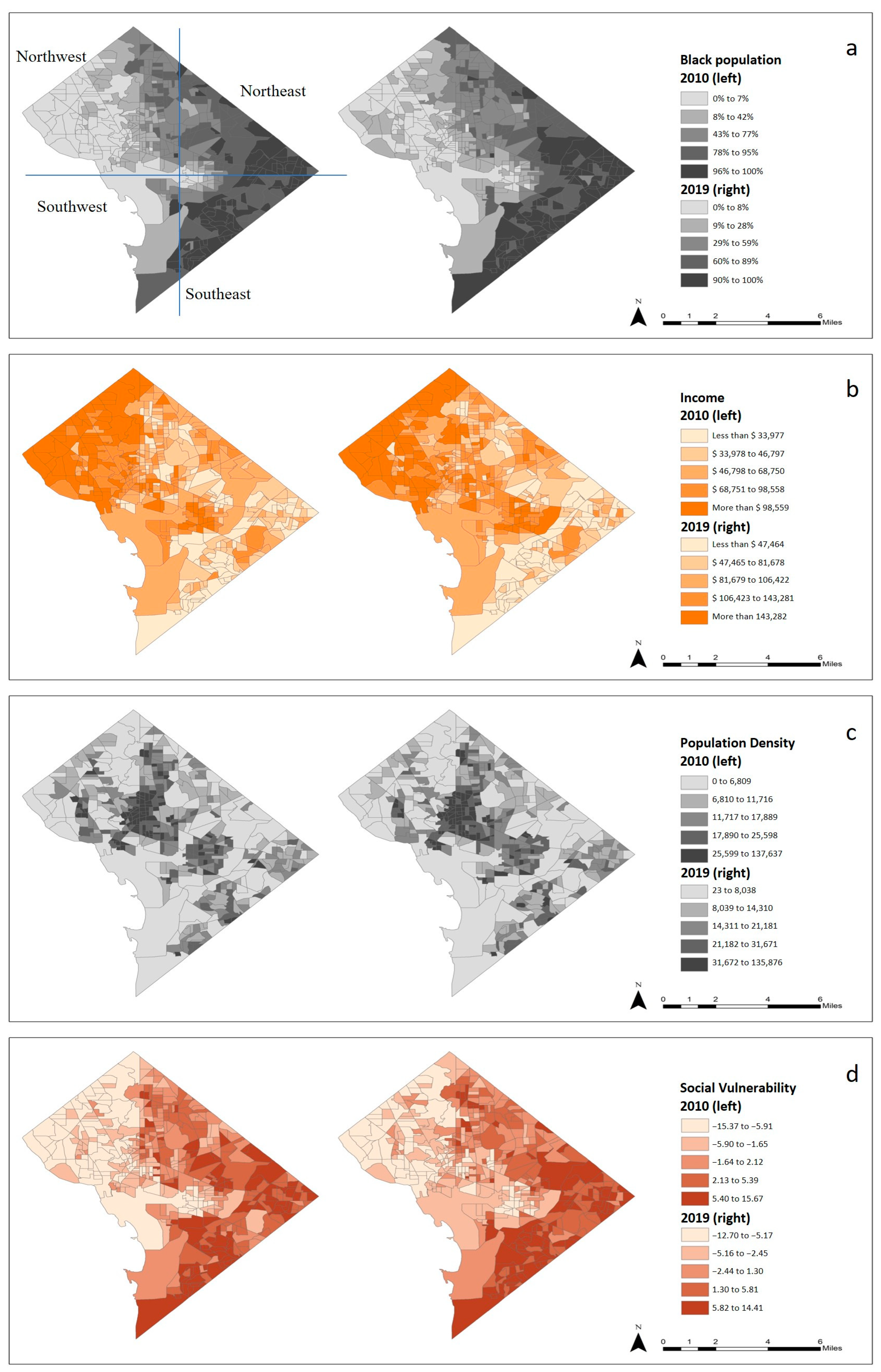
This research fills the significant gap by adopting a novel approach that explicitly considers the temporal dimension of GI distribution. Unlike previous studies that often rely on cross-sectional snapshots, this study employs a balanced panel data analysis, which allows for a comprehensive examination of how GI distribution evolves over time. By utilizing panel data, I capture the dynamics and trends that cross-sectional analyses may overlook, thus providing a more accurate representation of the changing landscape of GI distribution. Moreover, this study introduces a crucial and previously unexplored dimension by integrating a social vulnerability index into the analysis. While previous research has highlighted the unequal distribution of GI, our study goes beyond this by assessing the relationship between socioeconomic characteristics and GI distribution over time, especially in the context of socially vulnerable communities. This innovative approach helps identify areas that are most in need of GI investment, ensuring that the benefits of GI are directed toward the communities facing the greatest challenges.
This research seeks to address the following research question: Has the distribution of GI in Washington D.C. shown a tendency to concentrate more in communities with higher racial majorities and greater wealth? It addresses a pressing concern regarding the potential exacerbation of existing disparities in GI. By investigating this question, this study has the potential to inform policymakers, urban planners, and community stakeholders about the fairness and inclusivity of GI implementation. The results could lead to evidence-based policy recommendations that promote more equitable distribution strategies, ensuring that disadvantaged communities benefit from the positive impacts of GI. This article is organized as follows. First, the next section focuses on presenting the methodology adopted and specifics about the data used. Next, I show the main results obtained in the spatial panel regression analysis and present a discussion based on the temporal correlations between GI and socially vulnerable status. Thereafter, limitations, future research directions, and main conclusions are discussed.
3. Results
3.1. GI clustering
The interpretation of Univariate Local Moran’s I depends on the sign of the index and the significance level of the test. The statistic of the spatial autocorrelation suggests that the pattern of GIs at census block groups is clustered. The Moran’s Index is 0.371 with a z-score of 14.065, and the p-value is 0.001. Although it is difficult to say that there is a stronger clustering given that the value close to 1 indicates perfect clustering, the probability that the observed clustering pattern is due to random chance is less than 1 percent as the critical value is greater than 2.58.
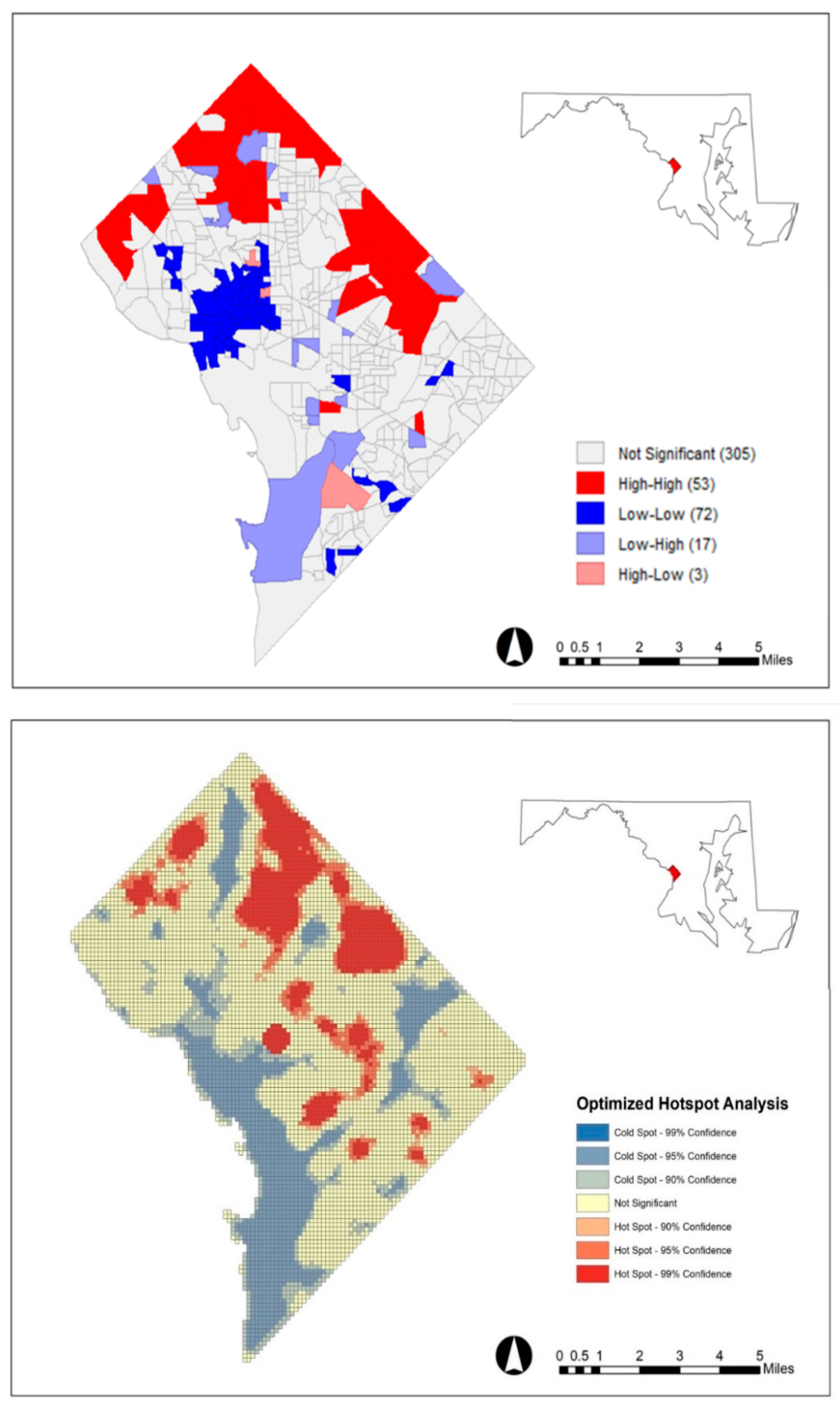
Additionally, the below cluster map identifies areas where there is a significant spatial concentration of high or low values of a variable of interest, which can provide insight into the spatial patterns (see
Figure 2). The presence of a high–high (HH) cluster on the LISA cluster map suggests that there is a spatial concentration of GIs in a specific area in D.C. Northeast and Northwest, where there are many GIs surrounded by neighboring areas with similarly high numbers of GIs. On the other hand, a low–low (LL) cluster in some communities in D.C. Southeast and around the National Mall indicates a spatial concentration of areas with fewer GIs, surrounded by neighboring areas with similarly low numbers of GIs. Overall, these patterns suggest that the concentration of GIs across D.C. varies across different spatial areas.
The optimized hot spot analysis also suggests that GIs in D.C. are clustering. If a z-score of Gi* statistic returned for each data cell of 500 feet by 500 feet is statistically significant and positive, it means that there is a strong clustering of high values, also known as a hot spot. In such cases, the larger the z-score, the stronger the clustering of high values. Conversely, if a z-score is statistically significant and negative, it means that there is a strong clustering of low values or a cold spot. In such cases, the smaller the z-score, the stronger the clustering of low values. Thus, the map output of the hot spot analysis illustrates that GIs are highly concentrated near the border of the Northeast and Northwest and in the Northeast. Although the concentration of GI is also observed in Southeast D.C., its size is much smaller than that of Northeast and Northwest D.C. The hot spot that exists around the central part of D.C. is a different point compared to the above cluster map. This reflects that analyzing the spatial clustering using Moran’s I can distort information about the true location of GI clusters.
Both the Univariate Local Moran’s I and the optimized hot spot analysis indicate that the pattern of GIs in D.C. is clustered. Although the two tools output different results regarding Southeast D.C., the LISA cluster map identifies significant clusters in the Northeast and Northwest, and the optimized hot spot analysis also shows that the GIs are highly concentrated in the same area of D.C. These results suggest that the concentration of GIs across D.C. varies across different spatial areas.
3.2. Spatial Panel Regression Results
The
Table 2 displays the Lagrange multiplier test results. The test includes SLM1, SLM2, and LM*-lambda conditional tests as proposed by Baltagi et al. [
39], which investigate the panel data regression model with spatial error correlation by combining ideas from two previous research strands. The output shows the statistically significant LM1 test statistic. The SLM1 is for testing spatial autocorrelation in linear regression models with random effects [
39], and thus the result indicates strong evidence against the null hypothesis of no spatial correlation in the model, in favor of the alternative hypothesis of random effects. Both SLM2 and the Conditional Lagrange Multiplier (LM*)-Lambda tests examine the presence of spatial autocorrelation in the specified regression model in which the dependent variable is cnt and the independent variables are sovi, popden, impvs, slope, and elev. Only with SLM2, researchers cannot exclude the possibility of incorrect inference when the “variance component” referring to the variability of the random effect is large [
38]. To address this issue, Baltagi et al. [
39] developed a conditional LM test that tests for the existence of spatial autocorrelation in the regression model while allowing for the possibility that the variance component may or may not be zero. Based on both test results, I can reject the null hypothesis of no spatial autocorrelation and conclude that there is evidence of spatial autocorrelation in the model.
The
Table 3 show the coefficients and statistical significance of a spatial panel regression model estimated using three different methods: Pooled OLS, Panel Spatial Autoregressive (SAR), and Panel Spatial Error Model (SEM). The analysis is based on a dataset with 4500 observations over a panel length of 10 years and 450 census block groups. The dependent variable is the annual increase in GI, and the independent variables are the social vulnerability index, population density, the proportion of imperviousness surface, the average slope of the community, and the average altitude of the community.
The results of the “locally robust panel Lagrange multiplier test” for spatial dependence [
38], which is based on the OLS estimation, show that there is strong evidence of spatial lag dependence, as the LM test statistic of 611.23 for spatial lag dependence has a very low
p-value (<2.2 × 10
−16). This suggests that the value of the dependent variable in each observation is spatially correlated with the value of the dependent variable in neighboring observations. Also, the locally robust LM test for spatial lag dependence supports this conclusion, with a statistic of a low
p-value of 5.418 × 10
−12. On the other hand, the LM test for spatial error dependence also has a statistically significant value of 564.21, indicating that there is evidence of spatial error dependence in the data. This means that the errors in the regression model are not independent, but rather, are correlated with the errors in neighboring observations. However, the locally robust LM test for spatial error dependence, which accounts for spatial heterogeneity, does not support the presence of spatial error dependence, as the
p-value is relatively high (0.4722). This may indicate that the spatial autocorrelation in the errors is not consistent across all observations, but rather varies locally.
Like these results, the coefficient of the spatial parameter ρ (spatial) is positive and statistically significant at the 1% level, indicating the presence of spatial autocorrelation in the data. On the other hand, the coefficient of the spatial parameter λ (error) is positive but not statistically significant, suggesting that the spatial errors are not systematically related to the independent variables. Additionally, the AIC and BIC values show that the Panel SAR model has the lowest information criteria, and the r-squared value of the SAR is slightly higher than the other two models. In sum, the results from the Lagrange multiplier test and the estimation of regression models indicate that the Panel SAR model is the best model among the three in terms of balancing goodness of fit and model complexity. The Panel SAR model accounts for the spatial autocorrelation between dependent variables by incorporating a spatial lag of the dependent variable in the regression equation, which would improve the accuracy of the parameter estimates, considering that the coefficient estimates for the annual Increase in GI in the Panel SAR model are smaller than the Pooled OLS and Panel SEM models.
The results show that the variables representing social vulnerability and population density are negatively associated with the annual increase in GI, and the coefficients are statistically significant at the 1% level in all three models. This analysis is a kind of panel regression, which reveals that a statistically significant negative coefficient means that as the independent variable increases within each individual entity over time, the dependent variable tends to decrease. Thus, the relationship implies that communities with much socially vulnerable or higher population density had experienced lower increases of GI annually, from 2010 to 2009. Also, considering that the SAR model is the best, the significant spatial parameter ρ means that the annual increase in GI in one census block group is positively correlated with the annual increase in GI in neighboring census block groups. In other words, the results suggest that neighboring communities’ increases in GI are affected by the annual increase in GI within their neighboring communities. Also, consider that the coefficient estimates for the annual increase in GI in the Panel SAR model are smaller than the Pooled OLS and Panel SEM models.
On the other hand, while the coefficients of the proportion of imperviousness surface, the average slope of the community, and the average altitude of the community are significant in the pooled OLS and the panel SEM, their influence on GI is not directly observable in the panel SAR model. The estimated effects of these independent variables may be overestimated or biased due to unobserved spatial factors in the pooled OLS and the panel SEM.
4. Discussion
4.1. Social Vulnerability and Green Infrastructure Growth
The analysis results indicate that communities with higher social vulnerability have experienced relatively fewer advancements or developments in terms of GI compared to other communities. This could imply that disparities in GI investment or development have persisted or even worsened for socially vulnerable communities during the 2010s. In other words, the communities that are more socially vulnerable have not seen as much progress in terms of increasing their GI compared to communities that are less vulnerable. This link between social vulnerability and GI growth has led to an uneven clustering of GIs across communities in Washington D.C., which carries significant implications for vulnerable groups during extreme weather conditions. The lack of sufficient GI in socially vulnerable communities can hinder their ability to adapt to changing climatic conditions and cope with the adverse effects of extreme weather events. In scenarios involving pluvial flooding or excessive heat, these deepening unequal distributions of GIs can result in varying levels of protection for different communities. Consequently, the exacerbation of disparities in GI development could lead to increased health disparities, reduced quality of life, and heightened social and economic vulnerabilities for these communities.
This disparity in protection can further exacerbate existing inequities during environmental extremes, as observed in previous disaster cases. Bolin and Kurtz [
25], Bullard [
33], and Fothergill and Peek [
28] demonstrate that individuals from groups already vulnerable before disaster experience relatively greater property damage and disproportionate support from societies during such events. This phenomenon intensifies the pre-existing socioeconomic disparities among communities.
Examining the aftermath of Hurricane Katrina in New Orleans allows us to dissect the specific mechanisms through which unequal infrastructure protection can heighten vulnerabilities and perpetuate long-standing patterns of marginalization. This focused approach facilitates drawing vital parallels between the New Orleans case and our current study area, shedding light on broader implications for urban planning and equity. Bullard [
33] delves into how factors such as race, socioeconomic status, and place intersected with environmental concerns during and after the disaster. Before Hurricane Katrina struck, African Americans in New Orleans settled in areas that were relatively more vulnerable to flooding within a discriminatory context, ultimately resulting in greater flood damage for them. However, Bullard [
33] argues that institutionalized racism played a role in the post-disaster processes of cleaning up, sheltering, providing housing, and levee protection. He asserts that they experienced discrimination during these processes. Specifically, this case illustrates how already vulnerable groups, once again, faced discrimination in protective measures of infrastructure after the disaster, ultimately placing them at greater risk once more. Bullard [
33] posits that the unequal protection from infrastructure in New Orleans can be traced back to historical, social, and political structures and institutions that have systematically maintained unequal access to resources and opportunities for disadvantaged populations. Socially vulnerable groups could be excluded or unrecognized in decision-making processes related to protective infrastructure or mitigation measures, which can lead to increased vulnerability to disasters and climate change. This suggests that socially vulnerable people may experience the perpetuation of historical patterns of marginalization through disaster events and inequitable infrastructure settings.
It is important to note that measures aimed at mitigating or adapting to climate change can, ironically, result in unintended consequences that exacerbate vulnerability. While these ‘good’ measures are often conceived with the intention of alleviating risk and vulnerability [
40], their practical impact may fall short of this goal if their distribution lacks equity, given that vulnerability is a relative concept [
31]. Reckien et al. [
41] assert that adaptation and mitigation policies may disproportionately affect vulnerable populations when not adequately designed. Thus, the introduction and implementation of mitigation or adaptation measures should not solely center on enhancing overall social vulnerability reduction and resilience at a citywide scale. Instead, they must also encompass considerations of potential discrimination against vulnerable groups or the exacerbation of their vulnerabilities. In other words, infrastructure development addressing climate change and disaster challenges necessitates more than just technical solutions. It involves decision-making processes, policies, and social contexts that influence the implementation and distribution of these measures. The presence of infrastructural disparities in certain neighborhoods is not due to a single event, act of discrimination, or capital improvement project [
42]. Rather, these disparities result from a series of entrenched obstacles woven into planning practices, policies, and implementation frameworks [
42]. I defer the investigation of this potential to be explored in future studies.
4.2. Higher Density and Green Infrastructure
The findings derived from the analysis unveil a significant and noteworthy negative correlation between population density and the annual growth of green infrastructure (GI) in the context of Washington D.C. This association underscores the potential challenges that arise when attempting to introduce and expand GI initiatives within densely populated urban environments. The observed negative relationship suggests that higher population densities within the city are intertwined with constraints on the adoption and integration of green infrastructure, primarily due to limitations in available land and restricted space for implementation. These limitations can impede the effective implementation of GI programs, resulting in an intricate interplay between the pressing need for urban sustainability and the inherent constraints posed by dense urbanization. Exploring innovative strategies for integrating green infrastructure within densely populated areas becomes paramount. Designing adaptable and space-efficient GI solutions that can thrive within the constraints of limited urban space holds promise for mitigating the challenges imposed by high population densities. Such strategies could encompass vertical greenery, rooftop gardens, pocket parks, and other creative approaches that optimize available space while enhancing urban livability and resilience.
Ferguson et al. [
43], Wolch et al. [
11], and McConnachie and Shacketon [
44] suggest that when investigating the reasons behind unequal green space access for certain racial groups, researchers are increasingly acknowledging that it is not just about any one factor in isolation. Rather, they are exploring how multiple elements converge to shape these disparities. Further investigation could delve into the potential ripple effects of the observed negative correlation. For instance, understanding how this relationship interacts with other socioeconomic factors, such as ethnicity and deprivation, could provide a deeper understanding of the complex dynamics underlying unequal green space access. This expanded analysis might shed light on whether certain demographic groups face compounded challenges due to the overlapping effects of multiple factors.
4.3. GI Clustering Mechanism and Policy Implications
The spatial autoregressive panel model accounts for spatial dependence in this panel dataset by introducing a spatial lag variable that reflects the average value of the dependent variable in neighboring units. That is, the results show that GI’s annual increase in a community is influenced not only by its own characteristics (here, social vulnerability and other independent variables) but also by neighboring communities’ GI increase. This spatial dependence between communities in GIs in part corresponds to Lim’s finding [
9] that the property owners’ voluntary participation in GI implementation is influenced by the locations of previous installations. However, his research was limited to voluntary GI implementation by property owners, which accounts for only 5012 of the total 33,813 GIs in D.C. as of 2022. Focusing solely on voluntary participation by property owners may not provide a complete picture of GI implementation patterns. A more comprehensive understanding of GI clustering is necessary to effectively address issues related to GIs and environmental justice. As Mandarano and Meenar [
10] noted, current GI programs in the United States, regardless of whether they are direct public investment, regulatory mandates, and incentives for voluntary implementation, require collaboration and engagement with communities and stakeholders and the capacity of communities, in terms of economic and political aspects, for effective implementation. Poor or racial minority communities often lack the capacity to get information about the incentives for GI, install GI on their properties, or engage in local decision-making processes, which indicates that GIs would cluster in wealthier and politically powerful communities as seen in the above results.
Promoting a more equitable distribution of GI has the potential to improve both capacity to weather extremes and social equity outcomes [
45]. For more equitable distribution of GIs in D.C., planners and engineers in the D.C. government need to become conscious of the current distribution of GIs and analyze the potentials of the distribution in reducing stormwater runoff or urban heat island effect, prioritizing equitable distribution of GIs across communities. To be specific, given that the current GI implementation inevitably leans on market forces [
6,
10], planners and engineers should also recognize that socially vulnerable people who lack social and economic resources can be excluded from the GI programs whether they are implemented by public or private and promote community engagement and participation in the decision-making process surrounding GI programs.
The concurrent efforts of several government agencies, including the District Department of Energy and Environment, D.C. Water, and the District Department of Transportation, to implement GI programs in Washington, D.C. is commendable. Their GI programs are designed to achieve a broad spectrum of program goals and offer numerous benefits, including increased sustainability and resilience. However, despite these efforts, it is unlikely that the current implementation of GI programs will properly achieve any one of those goals with regard to environmental justice due to the uneven distribution of GIs across communities. A more comprehensive approach is needed that integrates GI programs with other environmental justice initiatives, such as affordable housing and public transportation, to address the underlying social and economic inequalities that perpetuate environmental injustices [
11]. As suggested by Wolch et al. [
11], such an approach would be necessary to ensure that the benefits of GI are distributed equitably across communities, especially those that have been historically underserved. Therefore, a more holistic and integrated approach is needed to achieve true environmental justice and ensure that all communities in Washington, D.C. can reap the benefits of GI.
4.4. Limitations
There are several limitations in this study. In order to investigate the association between GI and independent variables, I utilized the count of GI units in each census block group as a proxy for the multifaceted capacity of GI. This approach was necessary due to the absence of variables in the raw GI data that could effectively represent its diverse functions. While the raw data did contain a value indicating retention or storage volume associated with stormwater processing, this value solely represented the capacity linked to stormwater management by the GI. Additionally, a significant portion (approximately 9%) of the retention volume data had null values, rendering it unsuitable for use. However, relying solely on the count of GI facilities within a given census block group as a stand-in for the true capacity of GI to manage stormwater or mitigate the heat island effect in that area might not accurately capture the complete extent of GI’s capabilities. GI is a heterogeneous form of infrastructure encompassing various types (such as bioswales, rain gardens, green roofs, and trees), which can be constructed in different sizes and locations within a given area. The effectiveness of GI in managing stormwater runoff or mitigating extreme heat can vary based on these factors. Consequently, additional interdisciplinary research is imperative to determine whether the distribution of GI considered in this study can genuinely represent the ability of communities’ green infrastructure to effectively address diverse weather extremes at the infrastructure level.
Furthermore, it should be noted that this study’s exclusive focus on Washington D.C. could be considered a limitation. While Washington D.C. serves as a suitable case study for exploring the connection between social vulnerability and GI distribution, its findings may not be directly transferable to other cities or regions due to the diverse programs being implemented for various purposes across different urban areas. The correlation between social vulnerability and GI distribution may exhibit variations in other urban locales, influenced by the distinct socioeconomic, environmental, and political factors that characterize each city. Similarly, the environmental and political considerations impacting GI distribution might diverge among urban regions, contingent upon localized policies, regulations, and stakeholder engagement. As a result, the applicability of this study’s findings beyond Washington D.C. could be constrained. Researchers who seek to investigate the relationship between social vulnerability and GI distribution in alternative cities or regions must consider these variations and contextual factors during their study’s design and analysis.
5. Conclusions
In conclusion, this study rigorously examined the relationship between social vulnerability and the annual increase in GI in Washington D.C. Through the application of a spatial panel dataset and advanced regression models, Pooled OLS, Panel Spatial Autoregressive (SAR), and Panel Spatial Error Model (SEM) were tested. Among the models, the Panel SAR approach proved most effective in explaining the observed dynamics and it was established that socially vulnerable communities and areas with higher population density experienced comparatively lower annual increases in GI. The presence of spatial parameters further emphasized that the annual increase in GI in one census block group positively influenced the increase in neighboring block groups.
These findings underscore an enduring nexus between social vulnerability and the disproportionate growth of GI, leading to varying levels of vulnerability during extreme weather events. This uneven distribution perpetuates disparities, wherein communities endowed with greater social and economic capital experience augmented protection, while their more vulnerable counterparts confront heightened susceptibility. These results may illuminate the pivotal roles played by the planning mechanism, particularly its reliance on infrastructure privatization, and the subsequent implementation mechanism. The unequal provision of infrastructure protection can be traced back to entrenched inequalities in access to resources and opportunities for marginalized populations [
33]. Additionally, a negative association between population density and the annual increase in GI highlights the challenges posed by limited space and competition for land use in densely populated areas.
Collectively, these findings underscore an urgent imperative to confront social vulnerability and champion an equitable distribution of GI. They accentuate the integral role of comprehensive urban planning and engineering practices in the effective implementation of GI programs. It is essential for planners and engineers to recognize the potential absence of incentives and engagement opportunities for socially vulnerable communities. Advocating for an equitable distribution of GI presents a pathway to fortify sustainability and advance social equity [
46]. To achieve this, planners should assess GI distribution through a lens of social vulnerability, thereby prioritizing communities in need. Moreover, the integration of GI with other environmental justice initiatives, encompassing affordable housing and public transportation, becomes imperative to ensure the even-handed dispersion of benefits [
11]. This study reaffirms the inescapable necessity for a comprehensive and integrated approach to secure equitable GI benefits across all communities in Washington, D.C.


