System Dynamics Tools to Study Mediterranean Rangeland’s Sustainability

Abstract

Rangelands are a key resource present all over the world and cover half of all emerged lands. They are even more important in drylands, where they cover 48% of the total area. Their intensification and the additional pressure added by climate change push these socio-ecological systems towards desertification. Over the last two decades, we have developed and applied System Dynamics (SD) models for the study of Mediterranean grasslands. In addition, we have designed procedures and analysis tools, such as global sensitivity analysis, stability analysis condition, or risk analysis, to detect the main drivers of these socio-ecological systems and provide indicators about their long-term sustainability. This paper reviews these works, their scientific background, and the most relevant conclusions, including purely technical and rangeland-related ones, as well as our experience as systemic modelers in a world driven by field specialists.

1. Introduction

Rangelands can be defined as those ecosystems where humans have managed their vegetation cover through the presence of livestock in order to obtain economic benefits [1]. This is the predominant land use in the world, occupying half of all emerged lands. Their extension is about 29 million km², of which 63% is located in drylands [2]. They cover about 70% of the needs of domestic ruminants [3] and are a key resource for developing countries, where they are the main support for the 1.2 billion people who survive on less than USD 1 a day [4].

The degradation of grazing systems can therefore affect large areas of the planet and the most vulnerable population. Many of these ecosystems are located on marginal, less fertile land, where increased livestock densities alter ecosystem structure and functions [5], leading to deterioration of their economic and biological productivity. The impact of grazing increases with aridity [6]. Substantial degradation is occurring across the world’s arid and semi-arid rangelands [7,8,9], and the expected increasing frequency and duration of droughts [7,10,11] and the foreseeable aridification of mid-latitudes [12,13], as a consequence of global warming, pose major threats to rangelands.

This work focuses on the Mediterranean region, where rangelands occupy 48% of the territory [14] and the threat of global warming is particularly acute [15,16]. In these ecosystems, the varied floristic diversity is noteworthy, including grasslands and meadows, which occupy 20% of the total [17], and more or less dense shrubs and forests where the main use is for livestock and the dominant species are goats and sheep. The abrupt land-use changes that were triggered in the Mediterranean in the middle of the last century are part of the Great Acceleration [18] and have had a major impact on rangelands. On the one hand, in a process that has advanced from north to south, agricultural systems have intensified due to technological possibilities that respond to the logic of the market. This has led to (i) higher stocking rates (a situation more noticeable on the southern shore of the Mediterranean Basin than in the north, where irrigation is a more characteristic feature of this intensification [19]; (ii) to the collapse of pastoral systems based on the movement of livestock (nomadism and transhumance) [20]; and (iii) to the massive use of animal feed [21,22]. On the other hand, large areas have been abandoned due to a rural exodus that concentrates the population in large cities [2].

The degradation of the Mediterranean rangelands belongs to the scope of desertification, since it occurs in drylands (specifically dry sub-humid, semi-arid, and arid areas) and is a consequence of climatic variations and economic activities, as states the United Nations definition of desertification [23]. Although some authors have questioned the possibility of desertification in Europe [24], the reality is that the European Union considers it a growing threat [25]. In countries such as Spain, agropastoral systems and abandoned rangelands are recognized as already degraded scenarios or at risk of desertification [26,27]. However, in southern Europe, the current threat of desertification is linked to macrofarms [28,29] and extensive livestock farming is more a solution than a problem [30].

This indicates that both desertification and rangeland use are complex issues. One of the main causes of quantitative and/or qualitative degradation is overgrazing as a result of increased livestock loading. Numerous works report the erosion processes triggered after the loss of plant cover, or the loss of fodder species [5,31,32,33,34]. Simultaneously, opposite forces operate in the territory, which allows us to glimpse that desertification is a complex phenomenon that requires a very fine adjustment in the intensity of land use. In fact, rural abandonment and, therefore, undergrazing, is another typical source of degradation in the northern Mediterranean. Shrub encroachment and the invasion of woody vegetation give rise to the so-called ‘green deserts’ [35], as unproductive, from a socio-economic point of view, as the territories where primary productivity has been reduced.

In addition, the rural outflow and lack of grazing that prevented the accumulation of plant biomass, has created enormous extensions of homogeneous forest masses with hardly any discontinuities with increased fuel loads [36], resulting in fire-prone landscapes [37], which combined with global warming, lead to increased higher fire risk, longer fire seasons, and more frequent large, severe fires [38,39,40]. Although low-intensity and low-frequency fires have always occurred naturally and play a regulatory role in Mediterranean ecosystems (against phytotoxic agents, promoting seed germination, etc.), when their virulence and recurrence increase (median fire return has been reduced from ~30 to ~10 years in some instances [41], they cause serious damage by exposing the soil to heavy rainfall, preventing seeders from replenishing seed banks [42], depleting re-sprouters bud banks [43], and/or favoring invasive species [44].

Modeling studies, while being a simplified representation of actual systems, can provide additional insights by allowing impact analyses of a wide range of farming practices and short- and long-term climate scenarios [45]. In particular, System Dynamics (SD) [46] has been used in the modeling of rangelands because of its ability to bring together the different aspects that concur in these socio-ecosystems. For example, several models have been developed on the relationships between environmental conditions and animal stocks [47,48,49,50,51,52,53,54], specifically taking into account the importance of livestock mobility in some cases [55]. Some studies incorporated economic components [56,57,58,59,60,61] and analyzed the economic effects of a public land policy [62,63] in their rangeland models of a livestock farm in developed countries. More recently, climate change has driven study on the impact of droughts in rangelands [45,64,65,66,67,68,69].

However, few studies [70,71] fill the gap between the biophysical relationships and socioeconomic behaviors. Hence, the economic and environmental importance of rangelands and the challenges they face (climate change, intensification, land-use change, or abandonment) is a relevant field of research [30,72,73], with growing concerns about the socioeconomic behaviors and decision making of farmers, such as profit-seeking behaviors [9,74,75,76,77,78,79]. Under the umbrella of this boy of research, here, (i) we point out the utilities of SD for tackling such a complex problem; (ii) we present the SD models developed for different cases of Mediterranean grasslands (Figure 1), paying special attention to dehesa rangelands, i.e., an agro-silvo-pastoral system resulting from the progressive clearing of the original forest of oaks and/or cork oaks and covering some 90,000 km² of the southwest of the Iberian Peninsula [78]; (iii) we describe the analysis procedures developed to study the stability of these socio-ecosystems and the factors that most influence it; and finally (iv), we present some of the main findings in the light of these analyses and modeling carried out.

2. An Appropriate Research Field for System Dynamics

The study of the sustainability of rangelands (or desertification, which would be its opposite) requires the use of comprehensive tools and a multidisciplinary approach, since various disciplines such as ecology, economics, or agronomy are involved in its understanding and management. The need for a holistic approach in complex socio-ecosystems is recurrent [79,80,81,82,83,84,85,86], and SD is a suitable tool for this challenge.

SD is a modeling methodology grounded on the theories of nonlinear dynamical systems and feedback control developed in mathematics, physics, and engineering. SD states that the main, but easily overlooked, cause of the behavior of a complex system lies in its underlying structure of relationships, which includes feedback loops, non-linear relations, delays, and decision rules. Formally, an SD model is a set of first-order ordinary differential equations that makes a stock-and-flow representation of the studied system; stock variables show the state of the system over time, and flow variables represent the processes that change the stocks [46,87]. The main advantages of SD [88,89]: (i) it improves system understanding, and develops system thinking skills, even from the first stage of its development as causal or sketch diagrams; (ii) SD models can incorporate empirical and process-based approaches, and help integrate interdisciplinary knowledge; (iii) the SD literature provides abundant information about related methodologies; and (iv) user-friendly software platforms allow easy access for non-modeler users.

The use of qualitative information is particularly useful in drylands where available data are limited [90]. SD is particularly useful when the system may face situations that have not previously occurred, i.e., its desertification. For such a task it is required to know the full range of behavior of the variables involved in the system. An example that can help to illustrate this critical aspect is the influence of soil quantity on biomass primary productivity (Figure 2). The loss of soil through erosion reduces the moisture content and availability of nutrients, and consequently the production of biomass falls. Usual information available to characterize the soil-productivity relationship covers the central part of the function, i.e., where the system is productive (red line in Figure 2). However, obtaining information on this function at the extremes is not so simple. It is in these uncomfortable parts of the function where the contribution of the SD is paramount, since it allows the implementation of hypotheses about how systems can work in critical situations that were initially inconceivable. On the one hand, we know that primary productivity will not grow indefinitely, however much soil there is, i.e., the function becomes saturated at some point. On the other hand, and this is where the problem of desertification lies, there will be a soil threshold below which the system becomes unproductive. Hence, at some point, the function becomes zero (Soil_min in Figure 2). As Sterman (2000) [87] puts it, the relationships between variables expressed by means of multiplicative factors are more realistic than their linear alternative when the equations are subjected to extreme conditions. This is precisely what happens when rangelands are degraded.

SD aims to build dynamic, complex, and comprehensive models capable of exploring the long-term impacts of alternative decisions, taking into account the laxity of the laws regulating the behavior of socio-ecological systems and the scarcity of data [91]. In addition, SD is a flexible enough tool to support different data sources and to accommodate multiple analyses. Thus, it is possible to use statistical or stochastic models within its structure and, as we will present later, program routines to implement advanced sensitivity analyses, optimizations, and probability calculations.

3. A Suite of Models for Assessing Rangeland Desertification

3.1. A Generic Desertification Model (GDM)

The conceptual paradigm of the SD models implemented to study rangeland stability is the classic models of predator–prey ecology of Lotka [92] and Volterra [93]. We have followed the work of Noy-Meir, who considered extensive livestock systems as a specific case of predator–prey systems [49,94], and those of Thornes [95,96], who addressed the study of erosion as an ecological relationship of competition for water between eroded soil and plant cover.

These ideas inspired the formulation of a GDM (see complete description in Ibáñez et al. (2008) [97]) that consists of an eight-equation dynamic model of a generic human–resource system. Briefly, the resource (N) plays the role of prey and the consumption units (U) that exploit it are the predators. The N renewal depends on the climate, the N stock, and a limiting factor (S), so called because its level is decisive for the survival of the exploited resource. Reciprocally, the level of N affects the regeneration of S, which also depends on U. In this way, S and N have a common destiny: if one does well, the other also does well, but if the degradation of one of them is triggered, then the other is also dragged along. The exploitation of N generates profits through a production function that also requires capital (K). As profit increases, so does U and N consumption; this mechanism also works in the opposite direction. The evolution of U, K, and N demand per unit of consumption follows a hill-climbing heuristic, i.e., is driven by the pursuit of a dynamic target (e.g., desired U) [87] that depends on profitability and, as in the case of U, on the opportunity cost (O), i.e., the average alternative rent outside the current economic activity.

The GDM supports the cyclical behavior of predators and prey. In nature, the increase in prey makes the predators grow at their expense reducing their number. When they run out of feed, the predator population falls and the prey population recovers, returning to the beginning of the cycle. However, the GDM can reproduce other types of dynamics. In the case of socio-ecological systems, the signs of scarcity are bypassed. The profit generated, which depends on prices, costs, and subsidies, allows using inputs that replace the lost resource (e.g., feed can replace the shortage of grass) and create a sense of prosperity even though the environment is degrading. Guided by a misleading abundance, the resource can be overexploited, hastening its degradation and causing irreparable damage to the system by crossing critical S thresholds (e.g., loss of fertile soil). This alternative behavior manifests itself in the form of unsustainable exponential growths that can lead to the collapse of the resource, that is, to the desertification of the system.

3.2. DESPAS Model

The adaptation of the GDM for the understanding of rangeland grazing, which seeks to study desertification processes due to overexploitation of pasturelands, gave rise to the DESPAS model (the Spanish acronym for desertification by overgrazing) [98,99]. The structure of DESPAS is shown in Figure 3. The model contemplates a single-species livestock herd composed of breeding females, (which serves as the capital, K, of the GDM) with mean and constant physiological states and nutritional requirements. The grass (the predatory resource) consumed by the animals is modulated by its availability. This function, called the functional response of livestock, can adopt various formulations [100] and determines, taking into account the animal’s energy requirements, the level of supplementary feeding required (see Section 3.3.3). It is assumed that these are commercial farms (GDM consumption units), and that all the animals meet their caloric needs in order to maximize their yield. Feed consumption determines the profit and loss account of the farm, since the expenditure on supplementary feeding is the most important. There is a feedback loop in which good economic results encourage the arrival of new farmers in the area or the intensification of the stocking density, leading to greater inputs of supplementary feed, reducing profits, and therefore discouraging the growth of livestock farming in the area.

The grass is composed of a single perennial species. Under this condition, along with the uniformity of climatic conditions assumed earlier, the primary production of grass can be satisfactorily represented by means of the logistic function. The outflows from this stock are grazing and grass decomposition, which are linearly proportional to the quantity of biomass present.

The reduction in plant cover due to grazing exposes the soil to the erosive effect of rain. Runoff, which is the erosive agent considered, depends on soil infiltration, the slope of the land, and soil erodibility [101,102,103]. The resulting relationship between plant cover and soil loss is compatible with those given by Elwell and Stocking (1976) [104], a robust empirical relationship in which erosion is maximum with bare soil and declines exponentially as plant cover increases.

Soil thickness depends on two other processes. On the one hand, soil formation from bedrock (weathering rate) and the decomposition of vegetation and, on the other, the leaching rate, i.e., the loss of water-soluble plant nutrients from the soil due to rain. The stock of this limiting factor determines grass productivity, forming a positive feedback mechanism between soil and vegetation. If the soil is kept above certain thicknesses, the system’s biomass productivity is reinforced: more soil > more fertility > more plant cover > more protection against erosion > more soil. However, if the soil begins to be lost, the direction of the loop is reversed (less soil > less vegetation cover > less soil), leading to the degradation of the vegetation–soil subsystem.

Changes in livestock stock are based on the economic rationality of the farmer: when the incomes exceed the costs per breeding female (which depend on the amount of supplementary feeding, i.e., the amount of grass consumed by the livestock) then the number of animals is increased and vice versa. Finally, destocking depends on the useful breeding life of females.

3.3. Extensions of the DESPAS Model

The design of a model depends on its purpose. This, however, may change over time as new situations arise. That is why DESPAS has been refined, extended, and sometimes even simplified in order to study different cases. The following sub-models have been implemented: (i) soil moisture, runoff production, and its erosive power; (ii) shrub–grass competition; (iii) supplementary feeding; (iv) farmers’ behavior; and (v) the price forming mechanism. In addition, we refer in this section to the temporal and special scales of the models. While the latter has been maintained in all the models, the different methodological developments and processes included have led us to modify the former.

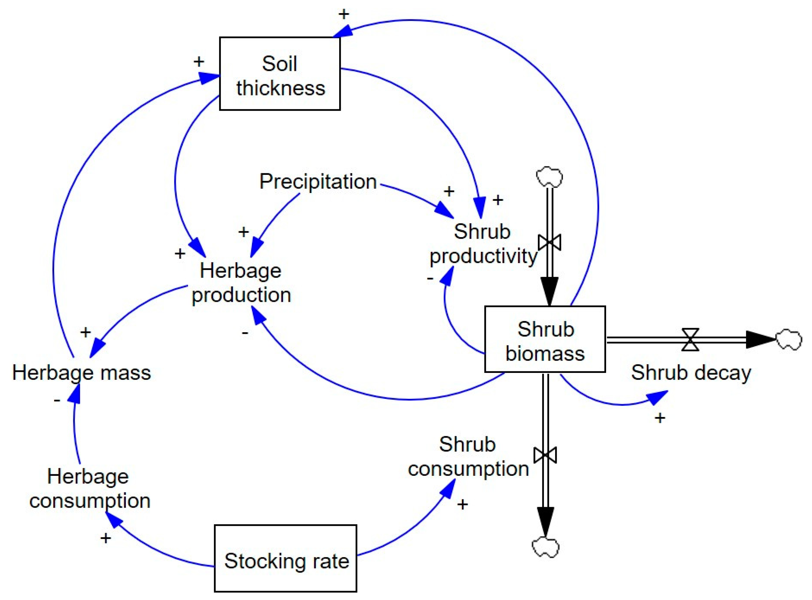
3.3.1. Soil Moisture, Runoff, and Erosion

In DESPAS, soil thickness is used as a limiting factor. However, in drylands, it is more accurate to use water as a limiting factor. For this purpose, the soil moisture level variable was included in the model [105,106]. This makes it possible to implement a water erosion mechanism (Figure 4) inspired by the analogy used by Thornes (1985) [95] to consider that runoff and soil compete for water. In fact, the better the soil absorption conditions and the more spaced the water falls, the less runoff is left to act as an erosive factor.

Soil moisture results from the balance between infiltration, evapotranspiration, and soil drainage; these three flows are naturally conditioned by the availability of water in the soil. The purpose of this water balance is to determine runoff; that is, water that cannot be trapped by soil pores and circulates freely on the surface. Runoff flow determines the rate of erosion.

The three initial flows are determined by two factors. First, they depend on the free space that the soil has to store the water. If all the pores of the soil are filled with water (soil moisture saturation) then there is no infiltration and all the water that falls becomes runoff and triggers soil erosion. Soil field capacity is the amount of soil moisture or water content held in soil after excess water has drained away; a sandy soil drains more water than a clay soil. Finally, the water used by the plants and reflected by the rate of evapotranspiration is the available water between the field capacity and the wilting point. The second factor is the rainfall torrentiality; i.e., how it is distributed over time. Even if the soil has a large storage capacity, if too much water falls in a short period of time, it cannot absorb it. On the other side, if the rain falls in a more distributed pattern (a lower torrential flow), then a greater fraction of the precipitation can be absorbed.

Finally, vegetation cover continues to play an essential role in erosion control. This is reflected in the model by considering that the infiltration rate is linked to the percentage of vegetation cover. Its protecting capacity follows the exponential behavior described in the previous section. The higher this is, the more precipitation is intercepted and retained, which translates into a greater infiltration rate.

The sub-model adds a further nuance to soil erosion, since it considers that the erosion rate decreases as soil is lost. In other words, the deeper layers of soil exposed by erosion are more compact because they contain fewer pores. Although this implies greater runoff, it also means that the erodibility of the soil is lower and therefore the erosion rate is reduced.

3.3.2. Shrub–Grass Competition

As mentioned above, the degradation of grazing areas in the Mediterranean has two opposing causes. DESPAS considers the most common, i.e., that overgrazing removes vegetation cover and triggers erosion rates. However, the excess of woody vegetation at the expense of pasture resulting from undergrazing is not sustainable either, since it does not allow livestock activity (in this sense, degradation is considered a loss of economic productivity). In both cases, the resulting degradation is difficult to reverse. On the one hand, the global average rate of soil formation is 0.036 mm per year [107], so that recovering 1 cm of soil takes 278 years. On the other hand, once perennial plants are able to establish themselves, they have an inherent advantage over annual plants at the beginning of the growing season. Since the latter have to restart their growth cycle from seed, they lose the competition for nutrients and light to established perennials, which emerge quickly from dormancy at the end of winter or a dry season [108].

We included the interaction between annual and perennial species (Figure 5) to enrich the behavior possibilities of the model and simulate shrub encroachment, which takes place in abandoned European rangelands [109]. For this purpose, herb productivity depends on shrub biomass through a multiplier. It considers that, in the absence of woody species, herb productivity is maximum (depending on rainfall and soil thickness), while as the proportion of woody species increases, annual herb productivity decreases until it is canceled out when woody plants have colonized all the available space. It was assumed that both annual and perennial herbs dry out at the end of the growing season (end of spring) and start growing again the next season (autumn) from seeds, roots, or underground stems. Since only aboveground biomass is considered and the time scale of the model is annual, no stock variable is needed for herbs, as they are annual plants.

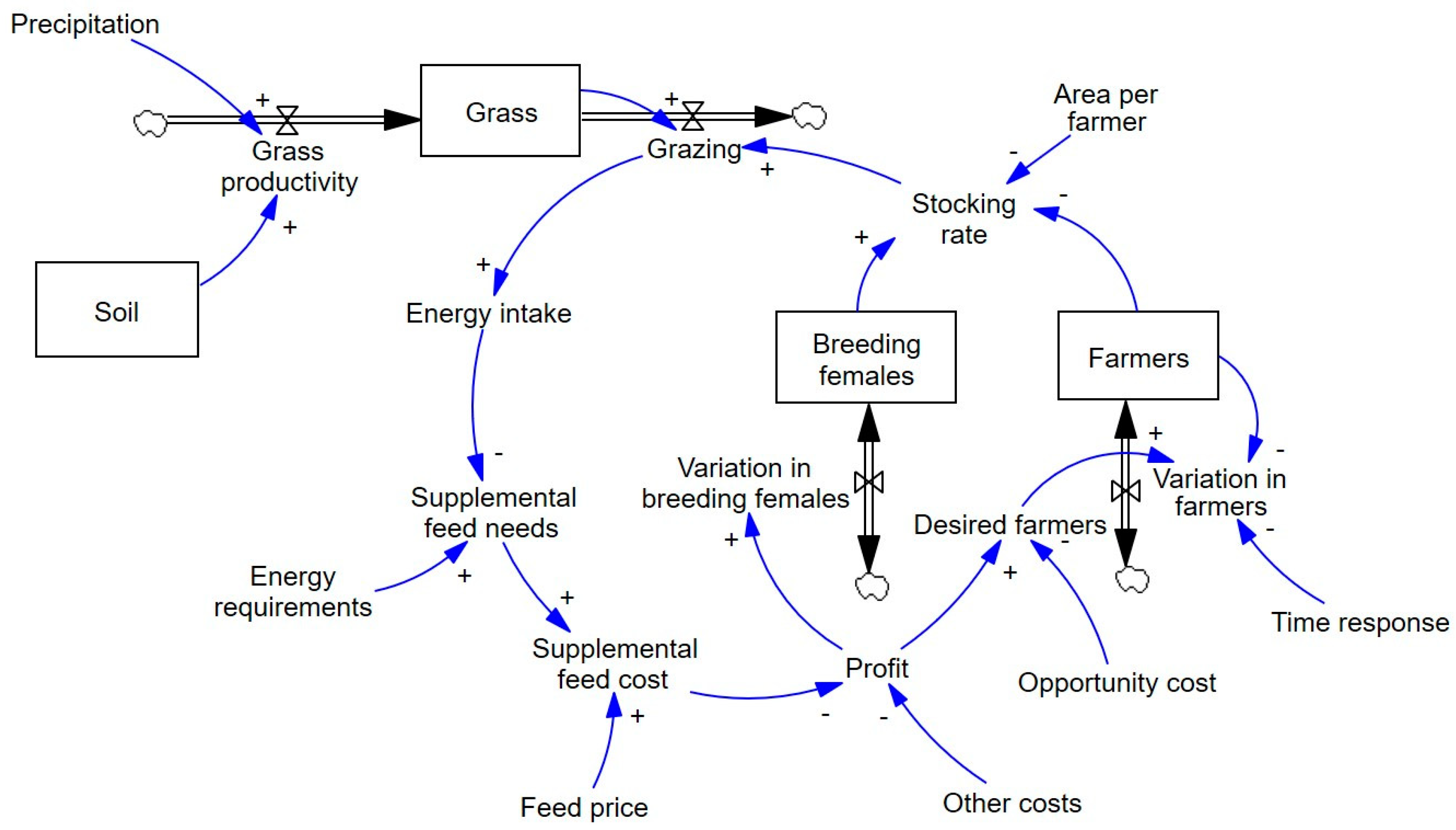
3.3.3. Supplementary Feeding

In commercial rangelands, one of the common strategies for coping with resource scarcity during dry seasons or droughts is the use of supplementary feeding. Sometimes, in addition, another drought-enduring strategy comes into play, such as allowing animals to lose weight during these shortages. Our model, however, assumes that all the energy requirements of the animals are always met and, for this purpose, there is a sub-model dedicated to calculating the amount of supplementary feed required and its cost.

Although the use of animal feed began as a temporary practice, it has been consolidated as a common practice that allows increasing the stocking rate. The basic structure of this sub-model is as follows (Figure 6): the energy gap resulting from the lack of pasture due to (i) the excessive presence of animals; (ii) drought periods; or (iii) reduced soil fertility due to erosion, increases the need for supplementary feeding. This has a negative impact on the benefit of the farmer, which should lead to a reduction in the stocking density. Relieving pressure on pasture leads to its recovery, which brings the situation back to the starting point; i.e., the animals would return to grazing exclusively on pasture and feed costs would disappear. However, fluctuations in feed prices can play an important role and allow for high stocking rates under scenarios of soil and pasture degradation. This sub-model presents one of the ways in which the scarcity signals of the territory are bypassed by the use of external inputs.

3.3.4. Farmers’ Behavior

One of the main assumptions of the GDM model is that consumption units (U)—the number of livestock farmers present in the area—depend on the profitability in relation to the opportunity cost; i.e., the alternative profit that would be obtained in another economic sector. To implement this hypothesis, the classical model of “goal-seeking” behavior [87] is used. The discrepancy between the current number of farmers (a stock variable) and the desired ones (the target in the goal-seeking model) is eliminated after a time delay by a positive or negative flow, depending on the sign of the discrepancy (note that this discrepancy is also dynamic, as the target changes) (Figure 6). Desired farmers depend on the profitability–opportunity cost ratio. The former variable is a function, in turn, of income and costs, which are built up from prices, subsidies, sales, and purchase volumes, which include the supplementary food item. The opportunity cost, on the other hand, can have a constant value or be a stochastic variable that follows an exponential probability distribution, i.e., the greater the opportunity cost, the less likely it is. This reflects well the fact that there are more economic actors with low opportunity costs, i.e., with alternative economic activities that offer a lower economic return than their current activity. The adjustment time of the function makes it possible to reflect the behavior of the economic agents involved. It can be more opportunistic (shorter delays) or conservative (longer delays).

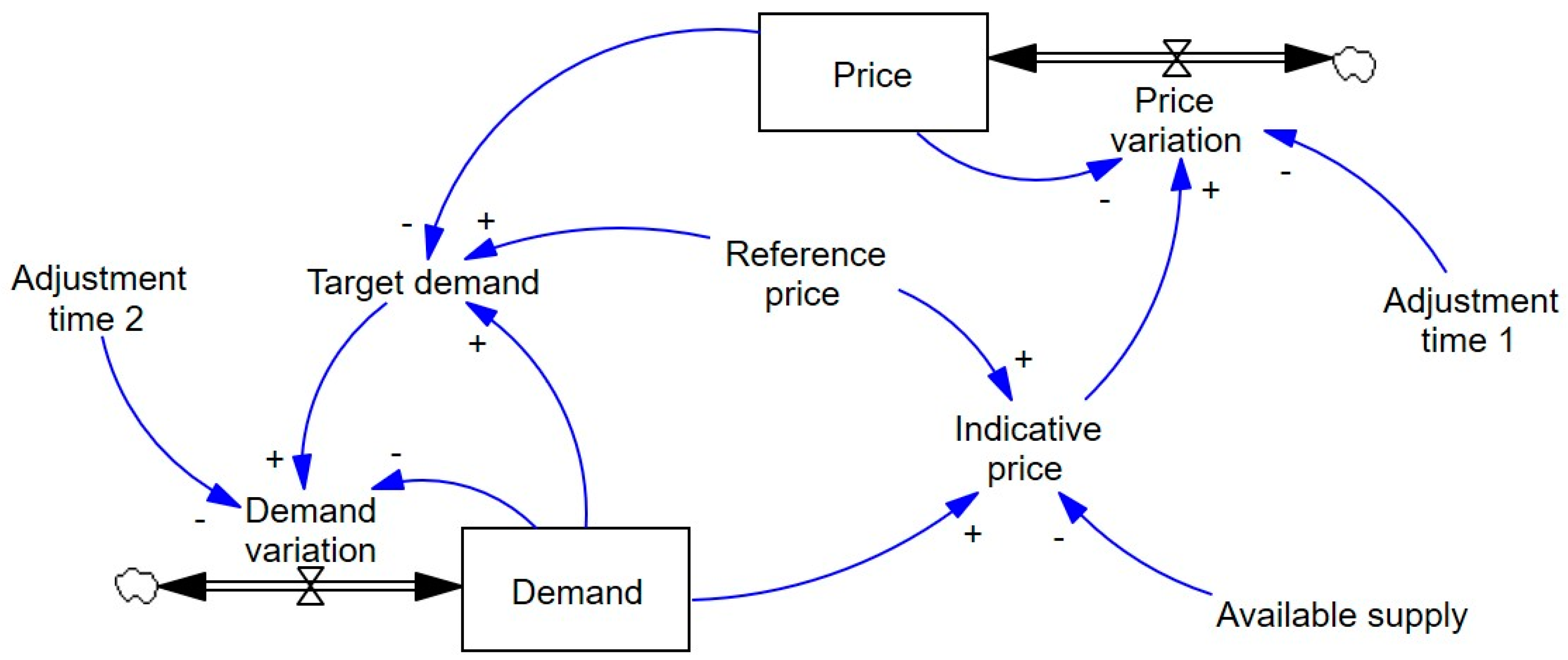
3.3.5. Price Forming Mechanism

In the initial versions of the DESPAS model, prices of inputs and outputs of the modeled goods are considered exogenous variables. However, this approach is not very realistic, since the price of raw materials is subject to changes derived from various circumstances, such as the current energy crisis. In addition, the internal dynamics of the system itself is responsible for changes in the prices of the products generated. Depending on the size of the livestock sector in the modeled area, the input and output market may be more or less influenced.

The price formation mechanism is similar for all commodities considered and it is represented in Figure 7. The sub-model assumes that farmers and traders lack complete knowledge of the system, so they use the hill-climbing heuristic to adjust their expectations to reality; i.e., the prices prevailing in the model at each instant are determined by the level variable “Price”. A reference price (which may be global or regional) and a price derived from the interplay of supply and demand are involved in the “Indicative price” setting. The product in question (feed, meat, etc.) evolves towards this price with a certain delay (“Adjustment time 1”).

The price, in turn, determines the “Target demand”, towards which the demand converges with another lag, the “Adjustment Time 2”. As demand changes, the indicative prices change, and so does the price. This simple structure is capable of generating a great complexity of behavior and, above all, eliminates the simplicity of considering that prices are fixed for the entire simulation period.

3.3.6. Temporal and Spatial Scales

Classical models of ecology do not refer to any specific spatial scale [110]. Our approach is, in this sense, more stringent, since the developed models refer to a spatial unit [89], such as a hectare, but do not distinguish between different parts within that space. The models presented in this section use superimposed two-time scales—short and medium term—to detail processes operating at different resolutions. First, the day is used to model the evolution of soil water, considering variables such as infiltration, saturation, runoff, and evapotranspiration. For purely operational reasons, the time unit is not exactly 1 day. The implementation of the models in the Vensim© software v.5.8 [111] makes it necessary to use time units (when the time unit is the year) that are a multiple of 2.85 days (≈0.0078125 years), as this is the minimum time step allowed by the program.

The year is used to represent processes occurring in the medium term, such as the evolution of the livestock population or the number of economic agents operating in the territory or their profits. Finally, the simulation periods cover several years, tens, or even centuries, since their purpose is to prospect the sustainability of the system, i.e., its long-term stability. For this purpose, it is necessary to study the behavior of variables whose dynamics are much slower (e.g., soil thickness, pasture productivity) and whose effect is felt over several decades.

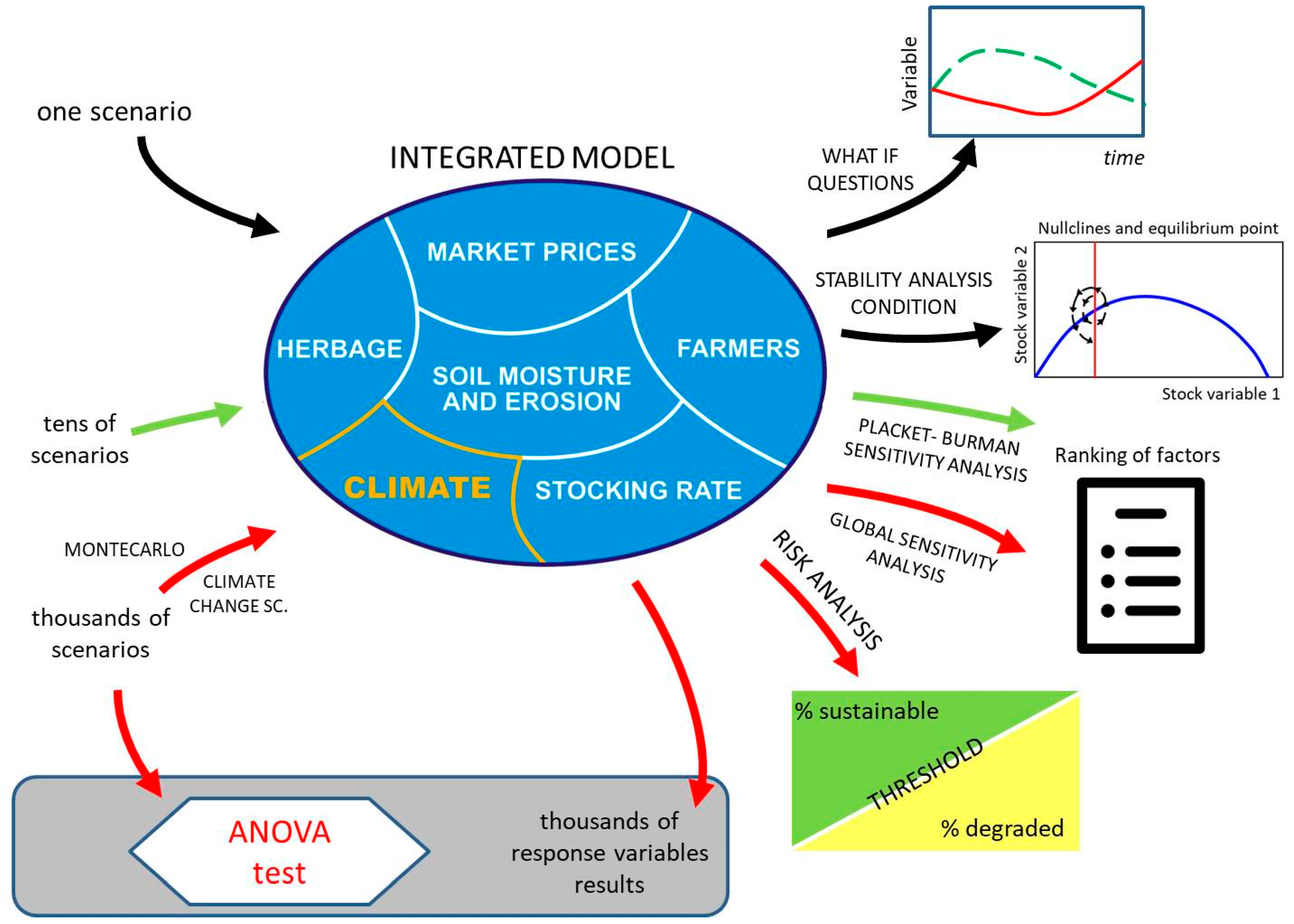
4. Design and Implementation of Analysis Tools to Explore Rangeland Behavior

In this section, we review the procedures we have designed and applied to analyze the modeled social-ecological systems. The exploitation of a model ranges from running a simple simulation scenario, which is the default use of an SD model, to the implementation of thousands of scenarios to rank the factors involved in a model (Figure 8). As these analyses become more sophisticated, programming routines are needed to automate the process of scenario creation and import, model simulation, and data export [112].

4.1. Temporal Trends and “What If” Questions

The standard output of SD models is the time trends of their variables (Figure 9). They respond to the scenario of simulation, i.e., the values of parameters and exogenous variables. Strictly speaking, these trajectories should not be considered predictions, since the background of the equations used is of a socio-ecological nature; i.e., they do not respond to laws of a physical and universal nature. Models that are founded on economic, social, and even biological formulations try to explore the future, but cannot forecast what will happen [113].

In this context, it is extremely useful to compare different scenarios, i.e., to answering ‘what if’ questions to analyze deviations from the baseline scenario. The following example (Figure 9) shows what would happen if subsidies were halved in Lagadas rangelands (Greece) [109]. As can be seen, the stocking rate is falling as the financial support is reduced (although not to the same extent), easing the pressure on the environment and slowing down erosion rates. In the absence of grazing, grasslands are invaded by woody species, which helps to protect the soil but at the same time reduces the productive capacity of grasslands.

Following the line of this exercise, it was interesting to look for the level of subsidy with which the erosion would be canceled. This would require a reduction in subsidies of up to 60%, which would mean a 26% drop in livestock (values not found in the historical record of the area) and a 30% decrease in the gross margin. According to these simulation results, it seems that erosion is inherent in grazing and that limiting soil erosion may in practice mean that farmers will have to close down their businesses.

4.2. Stability Analysis Condition

In order to gain a more precise idea of the long-term sustainability of grazing systems, it is possible to develop procedures that give us a more global vision than the more or less random simulation of scenarios. For this aim, the study of the stability of dynamic systems through the qualitative analysis of their equations [91,114] is the appropriate path to follow. Due to the uncertainty that is usually associated with the parametric values of many systems, and in particular, those referring to the natural environment [115,116,117], the qualitative analysis of a model can often be of greater interest than its quantitative results [118].

This methodological approach has been applied to dynamic predator–prey systems through the analysis of nullclines, both in linear [119] and non-linear [120] models and, more specifically, to ecological [121] and grazing systems [94,122]. A nullcline is defined as the equilibrium of a level equation (N); i.e., the equation resulting from performing dN/dt = 0. With them, it is possible to anticipate the behavior of a system in the long term by knowing the parametric values of the scenario and the initial values of the stock variables. This gives an idea of where the system is heading under current conditions, which serves as an early warning indicator.

Figure 10 shows the phase plane Pasture–Stocking rate, its nullclines, and the equilibrium point associated with its intersection. The stability of the equilibrium depends on the slope of the Pasture nullcline at the point of cut [122]. In this case, since the slope is positive, we are facing a stable equilibrium. To illustrate the use of these indicators, we used parametric scenarios to recreate three standard extensive livestock farming systems in Spain: cattle and sheep farmed on the dehesas and goats farmed on the south-eastern pastures [98,123].

4.3. Risk Analysis

The use of nullclines and graphical qualitative analysis is limited by the complexity of the model. Although it is possible to visualize three-dimensional isoclines [98,123], when the SD model has more than three level variables or the formulation of some nonlinear equation is intricate, it is not possible to obtain the nullclines equations. In this case, long-term equilibria are obtained by simulating the model with time horizons long enough to ensure the stabilization of the values. In addition, calculating the nullclines of a system means ‘freezing’ a scenario and assuming that everything will remain the same in the future. However, conditions fluctuate permanently.

To obtain a more precise idea of where the system is going, further equilibrium points can be calculated by varying the baseline scenario. These scenarios can be randomly generated using the Monte Carlo method by converting some model parameters into stochastic variables. For example, instead of using the mean precipitation, random values can be extracted from a stochastic variable that considers the mean and variance of precipitation. The procedure results in clouds of equilibrium points represented in a scatter plot (Figure 11). The dispersion of the cloud is critical to have a diagnosis. When it is high (Figure 11A), the system’s time-trajectory will wander rather erratically; if dispersion is low (Figure 11B), the time-trajectory will be more predictable.

To determine the risk of degradation, it is necessary to add degradation thresholds. Our role as modelers has often been to put these tools in the hands of specialists so that they can establish the thresholds they consider appropriate as well as other parametric values of the models. Additionally, to enrich the estimation of risks, the time needed to reach the defined thresholds is evaluated. Bear in mind that a model could show a desertification risk of 100%, but if it occurs after thousands of years (remember that the model simulates the time needed to reach a stable equilibrium), the risk may be negligible. To implement this idea, the model includes equations for computing the time the variables take to exceed their degradation thresholds. In this way, a probability of desertification will be obtained together with a “time to desertification” whose average will provide an estimate in each case.

The application of this methodology allowed the risk of desertification for the five “desertification landscapes” to be estimated [27,112,124] and included in the Spanish Action Plan against Desertification (SAPD; [26]). The results tell us that dehesas are one of the most sustainable land uses. Neither the soil nor the vegetation had an appreciable risk of deterioration over a 100-year time horizon, while for other desertification landscapes, such as groundwater-dependent irrigation systems, the results show that the risk of desertification is 88.2%, and that it will take, on average, 47 years.

4.4. Ranking of Factors

One of the objectives of the models presented is to have a precise idea of the most important factors in the future of the system. Specifically, and within the framework of desertification, it is crucial to distinguish between anthropic and climatic causes [125]. The Plackett–Burman Sensitivity Analysis (PBSA) [126,127] is an excellent option for ranking the factors of a socio-ecological system. This is a sound statistical procedure that measures the effects of each parameter on the target variables in an efficient way in terms of the number of necessary scenarios. An important feature is that the effects of every parameter are not measured with the all-other-things-being-equal assumption but are averaged over variations made in all other parameters. PBSA also enables measuring two-way interactions of pairs of parameters; although, this option was not used in this case.

Fortunately, the analysis capacity of computers is no longer an excuse to simulate a large number of scenarios. This paves the way to implement much more robust and conclusive sensitive analysis, such as Global Sensitivity Analysis (GSA) [128,129]. The most common GSAs are variance-based methods, which decompose the variance of a target variable into terms corresponding to the different parameters and their interactions [130]. Through GSA, we evaluated the sensitivities of key endogenous factors to the same percentage variation in 70 factors, including economic and climate drivers. The analysis considered the behaviors of 288,000 variants of the modeled system, each under a different 300-year driver scenario [131].

Among the main conclusions reached through the establishment of rankings, we have been able to verify the supremacy of climatic factors over the rest. For example (see

Table 1. Ranking example for a PBSA conducted in a dehesa [105]. In this case, the objective variable was “Time to loss 20 cm of soil”. The higher the negative percentage (red cells) means that the time is shortened, i.e., that the process of soil loss is faster. Positive percentages (green cells) mean a delay in soil loss. As can be seen, the ranking is led by climatic parameters.

Parameter	Impact
Mean annual precipitation	−36.9%
Fraction of annual precipitation that fell in the humid season	−17.5%
Mean annual reference evapotranspiration	12.5%
Fraction of annual evapotranspiration in the wet season	12.2%
Initial mean runoff coefficient soil at wilting point	−9.5%
Coefficient of variation annual precipitation	−8.1%
Coefficient of variation runoff coefficient soil at wilting point	−4.5%
Months when precipitation > ETo (length of the humid season)	2.4%
Total subsidies per hectare	−1.4%
Costs per female other than the cost of supplemental feed	1.3%
Mean meat price	−1.2%
Weathering rate of the parent rock	1.1%
Average number of years to form gross margin expectations	−0.5%
Mean price of supplemental feed	0.4%
Coefficient of variation supplemental feed	−0.2%
Coefficient of variation meat price	−0.2%
% Increase in breading females if gross margin increased by 10%	0.1%
Secondary income per breeding female	0.0%

for details), we found [105] that, when the “Mean annual precipitation” is increased by 10%, the time for the soil to be depleted was brought forward by 36.9%, while the effects for economic and behavioral variables were located in the lowest positions in the ranking. On the contrary, a 10% increase in “Mean meat price” delays time for the soil to be depleted only by −1.2%. The explanation for this result is strongly influenced by supplementary feeding, a common practice in commercial rangelands. Although this is one of the major costs of livestock farms, the farmer has enough financial margin to invest in feed and thus maintain production and, therefore, profit. Obviously, this situation may change if or when the prices of raw materials used to manufacture compound feed change.

4.5. Implementation of ANOVA Test

SD models can be used as virtual laboratories in which to conduct experiments [132]. In this context, a multi-way ANOVA test was coupled to an SD model to evaluate the sensitivity of a valuable type of commercial rangelands to increases in the frequency and intensity of droughts considering climate change scenarios [133]. In particular, the question is whether the current strategy of using feed to mitigate the effects of droughts will continue to be effective in the context of water scarcity that is expected to be particularly relevant in the Mediterranean [16].

For this purpose, 5400 simulation scenarios were generated from two blocking factors and two treatment factors. We have considered three Representative Concentration Pathway (RCP), i.e., scenario of future greenhouse gas emissions, and two downscaling methods, i.e., process by which coarse-resolution Global Climate Models outputs are translated into local climate information. Additionally, three levels were defined for the frequency and intensity of droughts. A hundred simulations (replicates) were run for each of the 3·2·3·3 = 54 cells in the analysis. These were obtained by varying the value of the random seed from 1 to 100.

The scenarios feed the model to generate results and after those inputs and outputs are used to implement the multi-way ANOVA test (see Figure 8, bottom). This has shown that most of the main effects and interactions turned out to be highly significant; although, the sensitivity of response variables to increases in the frequency and severity of droughts under climate change would be low or very low.

5. Findings through SD Modeling

5.1. Learnings from Mediterranean Rangelands Modeling

Agro-silvo-pastoral systems are one of the five desertification landscapes identified in the SAPD [26]. Our main conclusion in this context is that this land use presents a low risk of desertification [27,124]. This is due to the use of feed, which allows for mitigating the scarcity of pasture in dry periods [133]. Even in the context of climate change, with clear decreases in precipitation, it is estimated that the system will cope well with the shortage of pasture with the use of feed. Consistent with this conclusion, sensitivity analyses have revealed that climatic factors are more decisive than socio-economic factors [106]. This reinforces the validity of the use of feed as a drought-enduring strategy that safeguards the system.

However, we cannot think that the use of animal feed is a panacea. In northern Algeria, we have an example of how the progressive replacement of grass with cereal grain has led to the system’s collapse [134,135,136]. In these steppe rangelands, feed initially entered, as is often the case, as a punctual solution for extreme drought situations. Gradually, it became a regular supplement until national policies decided to turn the so-called Alfa seas (the name indicates the density of bushes in the region; Alfa is the name for the esparto grass, Macrochloa tenacissima) into an open-air farm. To this end, barley gradually replaced the country’s wheat fields. Through a state policy of subsidies, this barley is used to feed the increasingly numerous herds of the steppes. The main mistake was to ignore the sheep’s fiber needs, as barley only met their energy requirements. The consequences were devastating: thousands of hungry animals devoured the esparto grass, which was the shrub that helped alleviate periods of grass shortage. In the south of Oran, 700,000 ha out of 1.2 Mha of Alfa grass has completely disappeared and the remaining half million is much sparser (biomass was reduced from 1750 to 100 kg DM ha⁻¹) [137]. The loss of plant cover combined with the strong winds in the area has led to the appearance of dunes. This is a good example to illustrate that desertification is not the advance of a desert, but the creation of a desert-like landscape due to poor land management [138].

The livestock industry, which revolves around the use of compound feed, is a good example of global telecoupling [139], i.e., global supply chains involving large geographical distances and creating environmental pressures (including deforestation and other types of land conversions) remote from the places where the consumption of goods and services take place. Although industrial farming is the main consumer of feed, a more comprehensive assessment of the environmental impact of extensive farming may include the area of soybeans and cereal fields needed to supplement the animals’ diet. In the European case, the deforestation of primary forests in South America due to soy imports for feed compounds is especially relevant [140]. For the period 2000–2010, we have estimated that soybean consumption associated with the Spanish feed industry is equivalent to the deforestation of 1220 kha of primary ecosystems in South America, the main exporter of soybeans [141]. The models we have presented can be completed by incorporating the impact of feed consumption on the livestock farms studied in terms of area deforested.

Although socioeconomic drivers have less influence than climate drivers on the sustainability of the rangelands, there are many situations where their role is key. In Lagadas (Greece), we observed how the reduction in subsidies triggered the deterioration of the system [109]. Something similar to the Algerian case described above occurred. The rangeland scientists who helped us with that model expected that the cut in subsidies would lead to a reduction in livestock and thus slow down erosion. However, the model showed the opposite behavior. The conclusion seemed obvious to our colleagues: the model had to be wrong. Analyzing in depth the reasons for such unexpected behavior, we noticed that what was happening was that the livestock, although it was decreasing, did not do so in the proportion in which the subsidies did. Analyzing the causal tree, we could see that the reduction in subsidies meant a reduction in supplementary feeding but not to the same extent of the stocking rate. Consequently, the actual stocking rate was higher than in the baseline scenario, and therefore the animals were forced to consume more grass than was adequate, since the feed given was not sufficient to cover their needs.

Another relevant dynamic of the degradation of the Mediterranean grazing systems has to do with the economic behavior of farmers [142]. We have seen that a few opportunistic farmers, who only seek to maximize their profit by playing with the size of the herds, are enough to trigger degradation rates in the environment. The more cautious behavior of traditional farmers is only effective, in terms of rangeland sustainability, when it is highly dominant.

5.2. Multidisciplinarity: Under the Crossfire of Specialists

The scientific literature is full of recommendations about the need for multidisciplinary studies as the only way to address a multi-faceted and increasingly interconnected reality. Specifically, economics, combined with earth system sciences, is crucial for understanding both positive and negative impacts of alternatives and the trade-offs involved in a sustainable development path [143]. This is especially relevant to the serious environmental problems facing the planet, such as global warming, desertification, or loss of biodiversity. A more harmonious relationship between food systems and the ecological framework on which they are based is called for in order to achieve the Sustainable Development Goals [144]. As a result of this demand, numerous journals specializing in multidisciplinary approaches have emerged, and initiatives such as the EAT-Lancet [145], which bet on the systemic approach, have been launched. New paradigms have also emerged such as the socio-ecological systems [146], ecological economics [80], and the water–food–energy nexus [147], which try to give an integrated vision of nature and human beings.

Our experience during all these years has shown us that the integration of knowledge from different disciplines is difficult, to say the least. Inevitably, multidisciplinary work is evaluated by specialists in each of the subjects that are included in the integrated models. The problem is that, for a specialist, nothing is superfluous in his field and she/he declares she/himself incapable of judging and appreciating the added value of the contributions of other disciplines, which she/he does not know. Thus, for example, we find that an edaphologist misses, in the erosion sub-model, much more detailed equations, pointing out the impossibility of using point models, instead of spatially explicit ones, or considers unacceptable the simplification that involves ignoring the lithological characteristics of the terrain. However, it will be difficult to appreciate that this same model contains equations on the evolution of prices according to changes between supply and demand. Likewise, an economist will miss a more in-depth treatment of the profit and loss account, and a botanist may criticize the fact that the dynamics of each of the species that make up the pasture have not been treated separately. For both the economist and the botanist, it is likely to be superfluous to model runoff in order to calculate erosion rates.

Another practice that we have observed and that seriously penalizes the construction of integrated models is the growing refusal to review this type of work. Again, at least part of the explanation lies in the fact that the review work is carried out by specialists in the different disciplines that the model brings together, but who are not usually familiar with equations, much less with systems of differential equations. This task requires a great deal of time for understanding, as well as a minimum of mathematical knowledge. We are faced with judgments that again do not go beyond the boundaries of the reviewer’s discipline. At best, the reviewer assumes that a model with so many equations and references must be right (with all the vagueness that this judgment implies); at worst, the paper runs the risk of being rejected outright if the reviewer in question reads some detail that clashes with his or her perception of the subject.

In our case, we have had work rejected on the basis of arguments that demonstrate a lack of knowledge of the model. It has been said that the model is speculative (indeed it is, as is the case with any model based on a series of hypotheses or speculations), that the time horizons are excessive (in some cases, it is necessary to simulate the model for several hundred years in order to calculate equilibrium points of the system), that it is too simple (in models with more than eighty equations), or that the model is wrong because it does not reflect reality. In this last aspect, we agree since, in the end, “All models are wrong”, since they are deliberate simplifications of reality [148]. From our point of view, this type of judgment fits in perfectly with one of the obstacles Sterman points to in properly understanding complex dynamic systems [87]: unscientific reasoning, even among the scientific community itself.

There are notable exceptions to this discourse. For example, there are those who appreciate the connection of aspects as far apart, in principle, as subsidies and erosion rates. This is the culmination of the top-down approach of the systemic approach models. Indeed, one of the major achievements is to complete the model, in the sense of connecting all the elements of the system. It is obvious that these connections can be made more precise and improved over years. The important thing is to make the assumptions very clear and to return to these questions whenever possible and pertinent. On the contrary, the bottom-up approach, which is the immediate consequence of the reductionist approach of the scientific method, tries to aggregate particles of knowledge in such a way that a complex system is generated from the coupling of subsystems. As a consequence, its predictive capacity is quite high. However, this approach has a number of disadvantages [149] that are critical for our objectives: (i) they are models that need a large amount of data for their operation, which, in arid areas, is often not possible; (ii) there is a great risk of error propagation; and (iii) the strategy of trying to capture and replicate all kinds of processes makes bottom-up models hardly reach ‘the top’.

Over the years, we have found a number of specialists in fields such as hydrology, ecology, geography, or biology who have joined our working group and become enthusiastic advocates of the systemic approach. We must also acknowledge and thank the valuable contributions of reviewers from outside SD, which have allowed us to improve both models and manuscripts. One of the tools that are useful for involving participants from different disciplines and institutions is Decision Support Systems (DSS). These are very simple computer applications in which the user only has to press a series of buttons to execute tasks such as moving from one screen to another or performing more or less complex calculations. In our case, the DSS allow us to use Vensim© software v.5.8 [111] through Visual Basic. This opens the door to use a widely spread program such as Excel and to simulate SD models remotely, so that both scenarios and results are accessible from a spreadsheet.

DSS can play a key role in expanding scientific production to society, since it allows exploring, in a simple way, sophisticated simulation models and their results, involving the decision-making processes [150] and reducing the resistance that often produces environmental problems such as desertification [151]. Many of the methods developed during these fifteen years have been channeled into a DSS called SAT (the Spanish acronym for Early Warning System) [27,112,124]. SAT implements three SD models to cope with the five desertification landscapes described in the SPAD, two of which are related to the “rangelands affected by erosion” syndrome (Figure 12B). Despite their usefulness, we agree with Oxley (2004) [152] on the limited role of DSS and simulation models and that “decision-support for socio-natural systems is more fruitfully concerned with providing the political actors involved a means of exploration than a set of ‘definite’ solutions” [152].

6. Conclusions

Simulation models are a vital tool for understanding the multiple dynamics that converge on rangelands. This is the main land use in drylands and is key to the survival of the poorest countries. Over the course of two decades, we have developed integrated SD models to study Mediterranean rangelands and designed analytical tools coupled to them. Our goal was to understand the interactions between the different components of the system, to provide sustainability indicators, and to detect the main drivers of degradation of these socio-ecological systems.

Since the beginning of our research activity, we have addressed the study of rangelands from a holistic approach. Although multidisciplinarity in the study of socio-ecological systems is repeatedly advised, in many cases, the specialist’s point of view and reluctance to integrate knowledge from other disciplines still prevails. This is one of the burdens that the modeler must learn to bear, distinguishing constructive criticisms from those that only arise from those who refuse to leave their discipline of comfort and do not admit other points of view.

As we work on models, we encounter new challenges that call for new developments, which has led us to versions that incorporate new elements. Currently, two situations are of particular concern to us. On the one hand, the transformation of rangelands and silvo-pastoral dryland systems to croplands increases the risk of desertification due to increased pressure on the remaining rangelands or to the use of unsustainable cultivation practices. To address this problem, it is necessary to include other land-use dynamics, and one option is to link them with other models that we have implemented for other land uses, such as groundwater-dependent irrigation systems. On the other hand, we have to take into account the effects that move beyond the physical boundaries of rangelands due to feed consumption. These are some of the possible paths that models will follow. At the same time, new models usually require different analytical tools, which we have also been developing over the years.

In an increasingly complex world, it is mandatory to use tools that can deal with it. Simply pointing out the contradictions that arise in land use management and bringing them to the attention of stakeholders and politicians is, in our opinion, a valuable contribution.

References

1. Menke, J.; Bradford, G.E. Rangelands. Agric. Ecosyst. Environ. 1992, 42, 217–230. [Google Scholar] [CrossRef]
2. Cherlet, M.; Hutchinson, C.; Reynolds, J.; Hill, J.; Sommer, S.; Von Maltitz, G. (Eds.) World Atlas of Desertification; Publication Office of the European Union: Luxembourg, 2018; ISBN 978-92-79-75350-3. [Google Scholar]
3. Lund, G. Accounting for the World’s Rangelands. BioOne 2007, 29, 3–10. [Google Scholar] [CrossRef]
4. Bedunah, D.J.; Angerer, J.P. Rangeland Degradation, Poverty, and Conflict: How Can Rangeland Scientists Contribute to Effective Responses and Solutions? Rangel. Ecol. Manag. 2012, 65, 606–612. [Google Scholar] [CrossRef] [Green Version]
5. Asner, G.P.; Elmore, A.J.; Olander, L.P.; Martin, R.E.; Harris, A.T. Grazing Systems, Ecosystem Responses, and Global Change. Annu. Rev. Environ. Resour. 2004, 29, 261–299. [Google Scholar] [CrossRef]
6. Maestre, F.T.; Le Bagousse-Pinguet, Y.; Delgado-Baquerizo, M.; Eldridge, D.J.; Saiz, H.; Berdugo, M.; Gozalo, B.; Ochoa, V.; Guirado, E. Grazing and Ecosystem Service Delivery in Global Drylands. Science 2022, 378, 915–920. [Google Scholar] [CrossRef]
7. Maestre, F.T.; Eldridge, D.J.; Soliveres, S.; Sonia, K.; Delgado-baquerizo, M.; Bowker, M.A.; Garc, P.; Gait, J.; Gallardo, A.; Roberto, L. Structure and Functioning of Dryland Ecosystems in a Changing Structure and Functioning of Dryland Ecosystems in a Changing World. Annu. Rev. Ecol. Evol. Syst. 2016, 47, 215–237. [Google Scholar] [CrossRef] [Green Version]
8. Reynolds, J.F.; Smith, D.M.S.; Lambin, E.F.; Turner II, B.L.; Mortimore, M.; Batterbury, S.P.J.; Downing, T.E.; Dowlatabadi, H.; Fernandez, R.J.; Herrick, J.E.; et al. Global Desertification: Building a Science for Dryland Development. Science 2007, 316, 847–851. [Google Scholar] [CrossRef] [Green Version]
9. Allington, G.R.H.; Li, W.; Brown, D.G. Modeling System Dynamics in Rangelands of the Mongolian Plateau. In Proceedings of the Trans-disciplinary Research Conference: Building Resilience of Mongolian Rangelands, Ulaanbaatar, Mongolia, 9–10 June 2015; pp. 216–221. [Google Scholar]
10. Fu, Q.; Feng, S. Responses of Terrestrial Aridity to Global Warming. J. Geophys. Res. Atmos. 2014, 119, 7863–7875. [Google Scholar] [CrossRef]
11. Huang, J.; Yu, H.; Guan, X.; Wang, G.; Guo, R. Accelerated Dryland Expansion under Climate Change. Nat. Clim. Chang. 2015, 6, 166–172. [Google Scholar] [CrossRef]
12. Lin, L.; Gettelman, A.; Fu, Q.; Xu, Y. Simulated Differences in 21st Century Aridity Due to Different Scenarios of Greenhouse Gases and Aerosols. Clim. Chang. 2018, 146, 407–422. [Google Scholar] [CrossRef]
13. Park, C.-E.; Jeong, S.-J.; Joshi, M.; Osborn, T.J.; Ho, C.-H.; Piao, S.; Chen, D.; Liu, J.; Yang, H.; Park, H.; et al. Keeping Global Warming within 1.5 °C Constrains Emergence of Aridification. Nat. Clim. Chang. 2018, 8, 70–74. [Google Scholar] [CrossRef] [Green Version]
14. Le Houérou, H.N. Impact of Man and His Animals on Mediterranean Vegetation. In Mediterranean-Type Shrublands, Ecosystems of the World 11; Castri, F., Goodall, D., Specht, R., Eds.; Elsevier Science Publishers Co.: New York, NY, USA, 1981; pp. 479–521. [Google Scholar]
15. Samaniego, L.; Thober, S.; Kumar, R.; Wanders, N.; Rakovec, O.; Pan, M.; Zink, M.; Sheffield, J.; Wood, E.F.; Marx, A. Anthropogenic Warming Exacerbates European Soil Moisture Droughts. Nat. Clim. Chang. 2018, 8, 421–426. [Google Scholar] [CrossRef] [Green Version]
16. Cramer, W.; Guiot, J.; Fader, M.; Garrabou, J.; Gattuso, J.P.; Iglesias, A.; Lange, M.A.; Lionello, P.; Llasat, M.C.; Paz, S.; et al. Climate Change and Interconnected Risks to Sustainable Development in the Mediterranean. Nat. Clim. Chang. 2018, 8, 972–980. [Google Scholar] [CrossRef] [Green Version]
17. Papanastasis, V.P.; Mansat, P. Grasslands and related forage resources in Mediterranean areas. In Grasslands and Land Use Systems; Parente, G., Frame, J., Orsi, S., Eds.; Grassland Science in Europe, ERSA: Gorizia, Italy, 1996; Volume 1, pp. 47–57. [Google Scholar]
18. Steffen, W.; Broadgate, W.; Deutsch, L.; Gaffney, O.; Ludwig, C. The Trajectory of the Anthropocene: The Great Acceleration. Anthr. Rev. 2015, 2, 81–98. [Google Scholar] [CrossRef]
19. Puigdefábregas, J.; Mendizabal, T. Perspectives on Desertification: Western Mediterranean. J. Arid Environ. 1998, 39, 209–224. [Google Scholar] [CrossRef]
20. Liao, C.; Agrawal, A.; Clark, P.E.; Levin, S.A.; Rubenstein, D.I. Landscape Sustainability Science in the Drylands: Mobility, Rangelands and Livelihoods. Landsc. Ecol. 2020, 35, 2433–2447. [Google Scholar] [CrossRef]
21. Nefzaoui, A.; Ketata, H.; El Mourid, M. Changes in North Africa Production Systems to Meet Climate Uncertainty and New Socio-Economic Scenarios with a Focus on Dryland Areas. In New Approaches for Grassland Research in a Context of Climate and Socio-Economic Changes; Acar, Z., López-Francos, A., Porqueddu, C., Eds.; Options Méditerranéennes: Série A. Séminaires Méditerranéens; CIHEAM: Zaragoza, Spain, 2012; Volume 102, pp. 403–421. [Google Scholar]
22. Soto, D.; Infante-Amate, J.; Guzmán, G.I.; Cid, A.; Aguilera, E.; García, R.; González de Molina, M. The Social Metabolism of Biomass in Spain, 1900–2008: From Food to Feed-Oriented Changes in the Agro-Ecosystems. Ecol. Econ. 2016, 128, 130–138. [Google Scholar] [CrossRef]
23. UN (United Nations) United Nations Convention to Combat Desertification in Countries Experiencing Serious Drought and/or Desertification, Particularly in Africa. Document A/AC. 241/27, 12. 09. 1994 with Annexe; United Nations, New York. 1994. Available online: https://catalogue.unccd.int/936_UNCCD_Convention_ENG.pdf (accessed on 1 January 2023).
24. Mensching, H.G. Desertification in Europe? A Critical Comment with Examples From Mediterranean Europe. In Desertification in Europe; Fantechi, R., Margaris, N.S., Eds.; Springer: Dordrecht, The Netherlands, 1986; pp. 3–8. [Google Scholar]
25. European Court of Auditors. Combating Desertification in the EU: A Growing Threat in Need of More Action; European Court: Brussels, Belgium, 2018. [Google Scholar]
26. MAGRAMA. Programa de Acción Nacional Contra La Desertificación. Madrid; Ministerio de Agricultura y Medio Ambiente: Madrid, Spain, 2008.
27. Martínez-Valderrama, J.; Ibáñez, J.; Del Barrio, G.; Sanjuán, M.E.; Alcalá, F.J.; Martínez-Vicente, S.; Ruiz, A.; Puigdefábregas, J. Present and Future of Desertification in Spain: Implementation of a Surveillance System to Prevent Land Degradation. Sci. Total Environ. 2016, 563–564, 169–178. [Google Scholar] [CrossRef]
28. MITERD. Estrategia Nacional de Lucha Contra La Desertificación En España; Ministerio Para La Transición Ecológica Y El Reto Demográfico MITERD: Madrid, Spain, 2022.
29. Martínez-Valderrama, J.; del Barrio, G.; Sanjuán, M.E.; Guirado, E.; Maestre, F.T. Desertification in Spain: A Sound Diagnosis without Solutions and New Scenarios. Land 2022, 11, 272. [Google Scholar] [CrossRef]
30. Manzano, P.; Burgas, D.; Cadahía, L.; Eronen, J.T.; Fernández-Llamazares, Á.; Bencherif, S.; Holand, Ø.; Seitsonen, O.; Byambaa, B.; Fortelius, M.; et al. Toward a Holistic Understanding of Pastoralism. One Earth 2021, 4, 651–665. [Google Scholar] [CrossRef]
31. Ayoub, A.T. Extent, Severity and Causative Factors of Land Degradation in the Sudan. J. Arid Environ. 1998, 38, 397–409. [Google Scholar] [CrossRef]
32. Schnabel, S. Soil Erosion and Runoff Production in a Small Watershed under Silvo-Pastoral Landuse (Dehesas) in Extremadura, Spain; Geoforma Ediciones: Logroño, Spain, 1997. [Google Scholar]
33. Teketay, D. Deforestation, Wood Famine, and Environmental Degradation in Ethiopia’s Highland Ecosystems: Urgent Need for Action. Northeast. Afr. Stud. 2011, 8, 53–76. [Google Scholar] [CrossRef]
34. Wilcox, B.P.; Thurow, T.L. Emerging Issues in Rangeland Ecohydrology: Vegetation Change and the Water Cycle. Rangel. Ecol. Manag. 2006, 59, 220–224. [Google Scholar] [CrossRef]
35. Perevolotsky, A.; Seligman, N.G. Role of Grazing in Mediterranean Rangeland Ecosystems—Inversion of a Paradigm. Bioscience 1998, 48, 1007–1017. [Google Scholar] [CrossRef] [Green Version]
36. Moreira, F.; Rego, F.C.; Ferreira, P.G. Temporal (1958–1995) Pattern of Change in a Cultural Landscape of Northwestern Portugal: Implications for Fire Occurrence. Landsc. Ecol. 2001, 16, 557–567. [Google Scholar] [CrossRef]
37. Puigdefábregas, J. Erosión y Desertificación en España. Campo 1995, 132, 63–83. [Google Scholar]
38. Ruffault, J.; Moron, V.; Trigo, R.M.; Curt, T. Objective Identification of Multiple Large Fire Climatologies: An Application to a Mediterranean Ecosystem. Environ. Res. Lett. 2016, 11, 7. [Google Scholar] [CrossRef] [Green Version]
39. Turco, M.; Llasat, M.C.; Von Hardenberg, J.; Provenzale, A. Climate Change Impacts on Wildfires in a Mediterranean Environment. Clim. Chang. 2014, 125, 369–380. [Google Scholar] [CrossRef]
40. Tuel, A.; Eltahir, E.A.B. Why Is the Mediterranean a Climate Change Hot Spot? J. Clim. 2020, 33, 5829–5843. [Google Scholar] [CrossRef]
41. Syphard, A.; Radeloff, V.; Hawbaker, T.; Stewart, S. Conservation Threats Due to Human-Caused Increases in Fire Frequency in Mediterranean-Climate Ecosystems. Conserv. Biol. 2009, 23, 758–769. [Google Scholar] [CrossRef]
42. Zedler, P.H.; Gautier, C.R.; McMaster, G.S. Vegetation Change in Response to Extreme Events: The Effect of a Short Interval between Fires in California Chaparral and Coastal Scrub. Ecology 1983, 64, 809–818. [Google Scholar] [CrossRef]
43. Canadell, J.; López-Soria, L. Lignotuber Reserves Support Regrowth Following Clipping of Two Mediterranean Shrubs. Funct. Ecol. 1998, 12, 31–38. [Google Scholar] [CrossRef]
44. Arianoutsou, M.; Vilà, M. Fire and Invasive Plant Species in the Mediterranean Basin. Isr. J. Ecol. Evol. 2012, 58, 195–203. [Google Scholar]
45. Godde, C.M.; Garnett, T.; Thornton, P.K.; Ash, A.J.; Herrero, M. Grazing Systems Expansion and Intensification: Drivers, Dynamics, and Trade-Offs. Glob. Food Sec. 2018, 16, 93–105. [Google Scholar] [CrossRef]
46. Forrester, J.W. Industrial Dynamics; The MIT Press: Cambridge, MA, USA, 1961. [Google Scholar]
47. Moxnes, E. Overexploitation of Renewable Resources: The Role of Misperceptions. J. Econ. Behav. Organ. 1998, 37, 107–127. [Google Scholar] [CrossRef]
48. Badarch, D.; Ochirbat, B. On Sustainable Development of Cashmere Production and Goat Population in Mongolia. In Mongolian Studies at CNEAS. CNEAS Monograph Series 6; Oka, H., Ed.; Center for Northeast Asian Studies, Tohoku University: Sendai, Japan, 2002; pp. 187–200. [Google Scholar]
49. Noy-Meir, I. Grazing and Production in Seasonal Pastures: Analysis of a Simple Model. J. Appl. Ecol. 1978, 15, 809–835. [Google Scholar] [CrossRef]
50. Glasscock, S.N.; Grant, W.E.; Drawe, D.L. Simulation of Vegetation Dynamics and Management Strategies on South Texas, Semi-Arid Rangeland. J. Environ. Manag. 2005, 75, 379–397. [Google Scholar] [CrossRef]
51. Belcher, K.W.; Boehm, M. Evaluating Agroecosystem Sustainability Using an Integrated Model. In Managing for Healthy Ecosystems; Rapport, D.J., Lasley, B.L., Rolston, D.E., Ole Nielsen, N., Calvin, O., Qualset, A.B.D., Eds.; CRC Press (Taylor & Francis): Boca Raton, FL, USA, 2002; pp. 1209–1226. ISBN 978-0-42914-323-6. [Google Scholar]
52. Tedeschi, L.O.; Nicholson, C.F.; Rich, E. Using System Dynamics Modelling Approach to Develop Management Tools for Animal Production with Emphasis on Small Ruminants. Small Rumin. Res. 2011, 98, 102–110. [Google Scholar] [CrossRef] [Green Version]
53. Dace, E.; Muizniece, I.; Blumberga, A.; Kaczala, F. Searching for Solutions to Mitigate Greenhouse Gas Emissions by Agricultural Policy Decisions—Application of System Dynamics Modeling for the Case of Latvia. Sci. Total Environ. 2015, 527–528, 80–90. [Google Scholar] [CrossRef]
54. Moxnes, E.; Danell, Ö.; Gaare, E.; Kumpula, J. Optimal Strategies for the Use of Reindeer Rangelands. Ecol. Modell. 2001, 145, 225–241. [Google Scholar] [CrossRef]
55. Aderinto, R.F.; Ortega-s, J.A.; Anoruo, A.O.; Machen, R.; Turner, B.L. Can the Tragedy of the Commons Be Avoided in Common-Pool Forage Resource Systems? An Application to Small-Holder Herding in the Semi-Arid Grazing Lands of Nigeria. Sustainability 2020, 12, 5947. [Google Scholar] [CrossRef]
56. Hart, R.H.; Samuel, M.J.; Test, P.S.; Smith, M.A. Cattle, Vegetation, and Economic Responses to Grazing Systems and Grazing Pressure. J. Range Manag. 1988, 41, 282–286. [Google Scholar] [CrossRef]
57. Manley, W.A.; Hart, R.H.; Samuel, M.J.; Smith, M.A.; Waggoner, J.W.; Manley, J.T. Vegetation, Cattle, and Economic Responses to Grazing Strategies and Pressures. J. Range Manag. 1997, 50, 638–646. [Google Scholar] [CrossRef]
58. Ritten, J.P.; Bastian, C.T.; Frasier, W.M. Economically Optimal Stocking Rates: A Bioeconomic Grazing Model. Rangel. Ecol. Manag. 2010, 63, 407–414. [Google Scholar] [CrossRef]
59. Dunn, B.H.; Smart, A.J.; Gates, R.N.; Johnson, P.S.; Beutler, M.K.; Diersen, M.A.; Janssen, L.L. Long-Term Production and Profitability From Grazing Cattle in the Northern Mixed Grass Prairie. Rangel. Ecol. Manag. 2010, 63, 233–242. [Google Scholar] [CrossRef] [Green Version]
60. Turner, B.L.; Rhoades, R.D.; Tedeschi, L.O.; Hanagriff, R.D.; McCuistion, K.C.; Dunn, B.H. Analyzing Ranch Profitability from Varying Cow Sales and Heifer Replacement Rates for Beef Cow-Calf Production Using System Dynamics. Agric. Syst. 2013, 114, 6–14. [Google Scholar] [CrossRef]
61. Teague, W.R.; Kreuter, U.P.; Grant, W.E.; Diaz-Solis, H.; Kothmann, M.M. Economic Implications of Maintaining Rangeland Ecosystem Health in a Semi-Arid Savanna. Ecol. Econ. 2009, 68, 1417–1429. [Google Scholar] [CrossRef]
62. Torell, L.A.; Doll, J.P. Public Land Policy and the Value of Grazing Permits. West. J. Agric. Econ. 1991, 16, 174–184. [Google Scholar]
63. Torell, L.A.; Drummond, T.W. The Economic Impacts of Increased Grazing Fees on Gila National Forest Grazing Permittees. J. Range Manag. 1997, 50, 94–105. [Google Scholar] [CrossRef] [Green Version]
64. Baumgärtner, S.; Quaas, M.F. Ecological-Economic Viability as a Criterion of Strong Sustainability under Uncertainty. Ecol. Econ. 2009, 68, 2008–2020. [Google Scholar] [CrossRef] [Green Version]
65. Quaas, M.F.; Baumgärtner, S.; Becker, C.; Frank, K.; Müller, B. Uncertainty and Sustainability in the Management of Rangelands. Ecol. Econ. 2007, 62, 251–266. [Google Scholar] [CrossRef]
66. Freier, K.P.; Schneider, U.A.; Finckh, M. Dynamic Interactions between Vegetation and Land Use in Semi-Arid Morocco: Using a Markov Process for Modeling Rangelands under Climate Change. Agric. Ecosyst. Environ. 2011, 140, 462–472. [Google Scholar] [CrossRef]
67. Iglesias, E.; Báez, K.; Diaz-Ambrona, C.H. Assessing Drought Risk in Mediterranean Dehesa Grazing Lands. Agric. Syst. 2016, 149, 65–74. [Google Scholar] [CrossRef]
68. Gies, L.; Agusdinata, D.B.; Merwade, V. Drought Adaptation Policy Development and Assessment in East Africa Using Hydrologic and System Dynamics Modeling. Nat. Hazards 2014, 74, 789–813. [Google Scholar] [CrossRef]
69. Tinsley, T.L.; Chumbley, S.; Mathis, C.; Machen, R.; Turner, B.L. Managing Cow Herd Dynamics in Environments of Limited Forage Productivity and Livestock Marketing Channels: An Application to Semi-Arid Paci Fi c Island Beef Production Using System Dynamics. Agric. Syst. 2019, 173, 78–93. [Google Scholar] [CrossRef]
70. Oniki, S.; Shindo, K.; Yamasaki, S.; Toriyama, K. Simulation of Pastoral Management in Mongolia: An Integrated System Dynamics Model. Rangel. Ecol. Manag. 2018, 71, 370–381. [Google Scholar] [CrossRef]
71. Marandure, T.; Dzama, K.; Bennett, J.; Makombe, G.; Mapiye, C. Application of System Dynamics Modelling in Evaluating Sustainability of Low-Input Ruminant Farming Systems in Eastern Cape Province, South Africa. Ecol. Modell. 2020, 438, 109294. [Google Scholar] [CrossRef]
72. Herrero, M.; Thornton, P.K. Livestock and Global Change: Emerging Issues for Sustainable Food Systems. Proc. Natl. Acad. Sci. USA 2013, 110, 20878–20881. [Google Scholar] [CrossRef] [Green Version]
73. Briske, D.D.; Coppock, D.L.; Illius, A.W.; Fuhlendorf, S.D. Strategies for Global Rangeland Stewardship: Assessment through the Lens of the Equilibrium—Non-Equilibrium Debate. J. Appl. Ecol. 2020, 57, 1056–1067. [Google Scholar] [CrossRef]
74. Lubell, M.N.; Cutts, B.B.; Roche, L.M.; Hamilton, M.; Derner, J.D.; Kachergis, E.; Tate, K.W. Conservation Program Participation and Adaptive Rangeland Decision-Making. Rangel. Ecol. Manag. 2013, 66, 609–620. [Google Scholar] [CrossRef]
75. Marshall, N.A.; Stokes, C.J. Influencing Adaptation Processes on the Australian Rangelands for Social and Ecological Resilience. Ecol. Soc. 2014, 19, 14. [Google Scholar] [CrossRef]
76. Roche, L.M.; Schohr, T.K.; Derner, J.D.; Lubell, M.N.; Cutts, B.B.; Kachergis, E.; Eviner, V.T.; Tate, K.W. Sustaining Working Rangelands: Insights from Rancher Decision Making. Rangel. Ecol. Manag. 2015, 68, 383–389. [Google Scholar] [CrossRef]
77. Wilmer, H.; Fernández-Giménez, M.E. Rethinking Rancher Decision-Making: A Grounded Theory of Ranching Approaches to Drought and Succession Management. Rangel. J. 2015, 37, 517–528. [Google Scholar] [CrossRef]
78. Gea-Izquierdo, G.; Cañellas, I.; Montero, G. Acorn Production in Spanish Holm Oak Woodlands. Investig. Agrar. For. Syst. 2006, 13, 339–354. [Google Scholar] [CrossRef] [Green Version]
79. Liu, J.; Mooney, H.; Hull, V.; Davis, S.J.; Gaskell, J.; Hertel, T.; Lubchenco, J.; Seto, K.C.; Gleick, P.; Kremen, C.; et al. Systems Integration for Global Sustainability. Science 2015, 347, 1258832. [Google Scholar] [CrossRef] [PubMed] [Green Version]
80. Costanza, R. Ecological Economics: Reintegrating the Study of Humans and Nature. Ecol. Appl. 1996, 6, 978–990. [Google Scholar] [CrossRef] [Green Version]
81. Engler, J.O.; Von Wehrden, H. Global Assessment of the Non-Equilibrium Theory of Rangelands: Revisited and Refined. Land Use Policy 2018, 70, 479–484. [Google Scholar] [CrossRef]
82. Maestre, F.T.; Salguero-Gómez, R.; Quero, J.L. It Is Getting Hotter in Here: Determining and Projecting the Impacts of Global Environmental Change on Drylands. Philos. Trans. R. Soc. B Biol. Sci. 2012, 367, 3062–3075. [Google Scholar] [CrossRef] [PubMed] [Green Version]
83. Stafford Smith, D.M.; McKeon, G.M.; Watson, I.W.; Henry, B.K.; Stone, G.S.; Hall, W.B.; Howden, S.M. Learning from Episodes of Degradation and Recovery in Variable Australian Rangelands. Proc. Natl. Acad. Sci. USA 2007, 104, 20690–20695. [Google Scholar] [CrossRef] [Green Version]
84. Reynolds, J.F.; Stafford Smith, M. (Eds.) Do Humans Cause Deserts? In Global Desertefication. Do Human Cause Deserts; Dahlem University Press: Berlin, Germany, 2002; pp. 1–21. [Google Scholar]
85. Vetter, S. Rangelands at Equilibrium and Non-Equilibrium: Recent Developments in the Debate. J. Arid Environ. 2005, 62, 321–341. [Google Scholar] [CrossRef]
86. Liu, J.; Dietz, T.; Carpenter, S.R.; Alberti, M.; Folke, C.; Moran, E.; Pell, A.N.; Deadman, P.; Kratz, T.; Lubchenco, J.; et al. Complexity of Coupled Human and Natural Systems. Science 2007, 317, 1513–1516. [Google Scholar] [CrossRef] [Green Version]
87. Sterman, J.D. Business Dynamics: Systems Thinking and Modeling for a Complex World; Mc Graw Hill: New York, NY, USA, 2000; ISBN 0-07-231135-5. [Google Scholar]
88. Davies, E.G.R.; Simonovic, S.P. Global Water Resources Modeling with an Integrated Model of the Social-Economic-Environmental System. Adv. Water Resour. 2011, 34, 684–700. [Google Scholar] [CrossRef]
89. Kelly, R.A.; Jakeman, A.J.; Barreteau, O.; Borsuk, M.E.; ElSawah, S.; Hamilton, S.H.; Henriksen, H.J.; Kuikka, S.; Maier, H.R.; Rizzoli, A.E.; et al. Selecting among Five Common Modelling Approaches for Integrated Environmental Assessment and Management. Environ. Model. Softw. 2013, 47, 159–181. [Google Scholar] [CrossRef]
90. MEA (Millenium Ecosystem Assessment). Ecosystems and Human Well-Being: Desertification Synthesis; World Resources Institute: Washington, DC, USA, 2005. [Google Scholar]
91. Aracil, J. Introducción a La Dinámica de Sistemas; Alianza Editorial: Madrid, Spain, 1986. [Google Scholar]
92. Lotka, A.J. Elements of Mathematical Biology; Dover Publications: New York, NY, USA, 1956. [Google Scholar]
93. Volterra, V. Variations and Fluctuations of the Number of Individuals in Animal Species Living Together. In Animal Ecology; Chapman, B.M., Ed.; McGraw-Hill: New York, NY, USA, 1931; pp. 409–448. [Google Scholar]
94. Noy-Meir, I. Stability of Grazing Systems: An Application of Predator-Prey Graphs. J. Ecol. 1975, 63, 459–481. [Google Scholar] [CrossRef]
95. Thornes, J.B. The Ecology of Erosion. Geography 1985, 70, 222–235. [Google Scholar]
96. Thornes, J.B. Erosional Equilibria under Grazing. In Conceptual Issues in Enviromental Archaelology; Bintliff, J.L., Davidson, D.A., Grant, E.G., Eds.; Edinburgh University Press: Edinburgh, UK, 1988. [Google Scholar]
97. Ibáñez, J.; Martínez-Valderrama, J.; Puigdefábregas, J. Assessing Desertification Risk Using System Stability Condition Analysis. Ecol. Modell. 2008, 213, 180–190. [Google Scholar] [CrossRef] [Green Version]
98. Ibáñez, J.; Martínez-Valderrama, J.; Schnabel, S. Desertification Due to Overgrazing in a Dynamic Commercial Livestock-Grass-Soil System. Ecol. Modell. 2007, 205, 277–288. [Google Scholar] [CrossRef]
99. Martínez-Valderrama, J.; Ibáñez, J. Foundations for a Dynamic Model to Analyze Stability in Commercial Grazing Systems. In Sustainability of Agrosilvopastoral Systems—Dehesas, Montados; Schnabel, S., Ferreira, A., Eds.; Advances in Geoecology; International Union of Soil Sciences: Vienna, Austria, 2004; pp. 173–182. ISBN 3-923381-50-6. [Google Scholar]
100. Holling, C.S. The Components of Predation as Revealed by a Study of Small-Mammal Predation of the European Pine Sawfly. Can. Entomol. 1959, 91, 293–320. [Google Scholar] [CrossRef]
101. Band, L.E. Field Parameterization of an Empirical Sheetwash Transport Equation. Catena 1985, 12, 201–210. [Google Scholar] [CrossRef]
102. Kirkby, M.J. Soil Development Models as a Component of Slope Models. Earth Surf. Process. 1977, 2, 203–230. [Google Scholar] [CrossRef]
103. Thornes, J.B. The Interaction of Erosional and Vegetational Dynamics in Land Degradation: Spatial Outcomes. In Vegetation and Erosion; Thornes, J.B., Ed.; John Wiley & Sons: Chichester, UK, 1990; pp. 41–53. [Google Scholar]
104. Elwell, H.A.; Stocking, M. Vegetal Cover to Estimate Soil Erosion Hazard in Rhodesia. Geoderma 1976, 15, 61–70. [Google Scholar] [CrossRef]
105. Ibáñez, J.; Lavado Contador, J.F.; Schnabel, S.; Pulido Fernández, M.; Martínez-Valderrama, J. A Model-Based Integrated Assessment of Land Degradation by Water Erosion in a Valuable Spanish Rangeland. Environ. Model. Softw. 2014, 55, 201–213. [Google Scholar] [CrossRef]
106. Ibáñez, J.; Lavado Contador, J.F.; Schnabel, S.; Martínez-Valderrama, J. Evaluating the Influence of Physical, Economic and Managerial Factors on Sheet Erosion in Rangelands of SW Spain by Performing a Sensitivity Analysis on an Integrated Dynamic Model. Sci. Total Environ. 2016, 544, 439–449. [Google Scholar] [CrossRef] [PubMed]
107. Montgomery, D.R. Soil Erosion and Agricultural Sustainability. Proc. Natl. Acad. Sci. USA 2007, 104, 13268–13272. [Google Scholar] [CrossRef] [PubMed]
108. Tilman, D. Resource Competition and Community Structure; Princeton University Press: Princeton, NJ, USA, 1982. [Google Scholar]
109. Ibáñez, J.; Martinez-Valderrama, J.; Papanastasis, V.; Evangelou, C.; Puigdefabregas, J. A Multidisciplinary Model for Assessing Degradation in Mediterranean Rangelands. Land Degrad. Dev. 2014, 25, 468–482. [Google Scholar] [CrossRef]
110. Atanasova, N.; Džeroski, S.; Kompare, B.; Todorovski, L.; Gal, G. Automated Discovery of a Model for Dinoflagellate Dynamics. Environ. Model. Softw. 2011, 26, 658–668. [Google Scholar] [CrossRef]
111. Ventana Systems Inc. VensimDSS. 2019. Available online: https://www.ventanasystems.com/software/ (accessed on 1 January 2023).
112. Martínez-Valderrama, J.; Ibáñez, J.; Alcalá, F.J.; Martínez, S. SAT: A Software for Assessing the Risk of Desertification in Spain. Sci. Program. 2020, 2020, 7563928. [Google Scholar] [CrossRef]
113. Perry, G.L.W.; Millington, J.D.A. Spatial Modelling of Succession-Disturbance Dynamics in Forest Ecosystems: Concepts and Examples. Perspect. Plant Ecol. Evol. Syst. 2008, 9, 191–210. [Google Scholar] [CrossRef]
114. May, R.M. Thresholds and Breakpoints in Ecosystems with a Multiplicity of Stable States. Nature 1977, 269, 471–477. [Google Scholar] [CrossRef]
115. Frank, P.M. Introduction to System Sensitivity Theory; Academic Press: New York, NY, USA, 1978; ISBN 978-0-12265-650-7. [Google Scholar]
116. Swart, J. Sensitivity of a Hyrax-Lynx Mathematical Model to Parameter Uncertainty. South Afr. J. Sci. 1987, 83, 545–547. [Google Scholar]
117. Van Coller, L. Automated Techniques for the Qualitative Analysis of Ecological Models: Continuous Models. Conserv. Ecol. 1997, 1, 5. [Google Scholar] [CrossRef] [Green Version]
118. Martínez-Vicente, S.; Requena, A. Dinámica de Sistemas. 1. Simulación Por Ordenador; Alianza Editorial: Madrid, Spain, 1986. [Google Scholar]
119. Rosenzweig, M.L.; MacArthur, R.H. Graphical Representation and Stability Conditions of Predator-Prey Interactions. Am. Nat. 1963, 97, 209–223. [Google Scholar] [CrossRef]
120. Edelstein-Keshet, L. Mathematical Models in Biology; The Random House: New York, NY, USA, 1988. [Google Scholar]
121. Holling, C.S. Resilience and Stability of Ecological Systems. Annu. Rev. Ecol. Syst. 1973, 4, 1–23. [Google Scholar] [CrossRef] [Green Version]
122. Gotelli, N.J. A Primer in Ecology, 2nd ed.; Sinaver Associates Inc. Publishers: Sunderland, MA, USA, 1998. [Google Scholar]
123. Martínez-Valderrama, J. Análisis de La Desertificación Por Sobrepastoreo Mediante Un Modelo de Simulación Dinámico; Universidad Politécnica de Madrid: Madrid, Spain, 2006. [Google Scholar]
124. Ibáñez, J.; Martínez-Valderrama, J.; Martínez Vicente, S.; Martínez Ruiz, A.; Rojo Serrano, L. Procedimientos de Alerta Temprana y Estimación de Riesgos de Desertificación Mediante Modelos de Dinámica de Sistemas; Ministerio de Agricultura, Alimentación y Medio Ambiente: Madrid, Spain, 2015; ISBN 978-84-491-0074-1.
125. Xu, D.; Li, C.; Zhuang, D.; Pan, J. Assessment of the Relative Role of Climate Change and Human Activities in Desertification: A Review. J. Geogr. Sci. 2011, 21, 926–936. [Google Scholar] [CrossRef]
126. Plackett, R.L.; Burman, J.P. The Design of Optimum Multifactorial Experiments. Biometrika 1946, 33, 305–325. [Google Scholar] [CrossRef]
127. Beres, D.L.; Hawkins, D.M. Plackett–Burman Technique for Sensitivity Analysis of Many-Parametered Models. Ecol. Modell. 2001, 141, 171–183. [Google Scholar] [CrossRef]
128. Gan, Y.; Duan, Q.; Gong, W.; Tong, C.; Sun, Y.; Chu, W.; Ye, A.; Miao, C.; Di, Z. A Comprehensive Evaluation of Various Sensitivity Analysis Methods: A Case Study with a Hydrological Model. Environ. Model. Softw. 2014, 51, 269–285. [Google Scholar] [CrossRef] [Green Version]
129. Saltelli, A.; Ratto, M.; Andres, T.; Campolongo, F.; Cariboni, J.; Gatelli, D.; Saisana, M. Global Sensitivity Analysis: The Primer; John Wiley & Sons: Chichester, UK, 2008. [Google Scholar]
130. Sobol, I.M. Global Sensitivity Indices for Nonlinear Mathematical Models and Their Monte Carlo Estimates. Math. Comput. Simul. 2001, 55, 271–280. [Google Scholar] [CrossRef]
131. Ibáñez, J.; Martínez-Valderrama, J.; Contador, J.F.L.; Fernández, M.P. Exploring the Economic, Social and Environmental Prospects for Commercial Natural Annual Grasslands by Performing a Sensitivity Analysis on a Multidisciplinary Integrated Model. Sci. Total Environ. 2020, 705, 135860. [Google Scholar] [CrossRef]
132. Potkonjak, V.; Gardner, M.; Callaghan, V.; Mattila, P.; Guetl, C.; Petrović, V.M.; Jovanović, K. Virtual Laboratories for Education in Science, Technology, and Engineering: A Review. Comput. Educ. 2016, 95, 309–327. [Google Scholar] [CrossRef] [Green Version]
133. Martínez-Valderrama, J.; Ibáñez, J.; Ibáñez, M.A.; Alcalá, F.J.; Sanjuán, M.E.; Ruiz, A.; Del Barrio, G. Assessing the Sensitivity of a Mediterranean Commercial Rangeland to Droughts under Climate Change Scenarios by Means of a Multidisciplinary Integrated Model. Agric. Syst. 2021, 187, 103021. [Google Scholar] [CrossRef]
134. Martínez-Valderrama, J.; Ibáñez, J.; Del Barrio, G.; Alcalá, F.J.; Sanjuán, M.E.; Ruiz, A.; Hirche, A.; Puigdefábregas, J. Doomed to Collapse: Why Algerian Steppe Rangelands Are Overgrazed and Some Lessons to Help Land-Use Transitions. Sci. Total Environ. 2018, 613–614, 1489–1497. [Google Scholar] [CrossRef] [PubMed]
135. Hirche, A.; Salamani, M.; Abdellaoui, A.; Benhouhou, S.; Martínez-Valderrama, J. Landscape Changes of Desertification in Arid Areas: The Case of South-West Algeria. Environ. Monit. Assess. 2011, 179, 403–420. [Google Scholar] [CrossRef]
136. Slimani, H.; Aidoud, A. Desertification in the Maghreb: A Case Study of an Algerian High-Plain Steppe. In Environmental Challenges in the Mediterranean 2000–2050; Marquina, A., Ed.; Kluwer Academic Publishers: Amsterdam, The Netherlands, 2004; pp. 93–108. [Google Scholar]
137. Aidoud, A. Vegetation Changes and Land Use Changes in Algerian Steppe Rangelands. In Restauración de la Cubierta Vegetal en Ecosistemas Mediterráneos; Pastor-López, A., Seva-Román, E., Eds.; Instituto de Cultura Juan-Gil Albert: Alicante, Spain, 2002; pp. 53–80. [Google Scholar]
138. Martínez-Valderrama, J.; Guirado, E.; Maestre, F.T. Unraveling Misunderstandings about Desertification: The Paradoxical Case of the Tabernas-Sorbas Basin in Southeast Spain. Land 2020, 9, 269. [Google Scholar] [CrossRef]
139. Yu, Y.; Feng, K.; Hubacek, K. Tele-Connecting Local Consumption to Global Land Use. Glob. Environ. Chang. 2013, 23, 1178–1186. [Google Scholar] [CrossRef]
140. WWF (World Wildlife Fund). The Growth of Soy: Impacts and Solutions; WWF: Gland, Switzerland, 2014. [Google Scholar]
141. Martínez-Valderrama, J.; Sanjuán, M.E.; Barrio, G.; Guirado, E.; Ruiz, A.; Maestre, F.T. Mediterranean Landscape Re-Greening at the Expense of South American Agricultural Expansion. Land 2021, 10, 204. [Google Scholar] [CrossRef]
142. Ibáñez, J.; Martínez-Valderrama, J. Global Effectiveness of Group Decision-Making Strategies in Coping with Forage and Price Variabilities in Commercial Rangelands: A Modelling Assessment. J. Environ. Manag. 2018, 217, 531–541. [Google Scholar] [CrossRef] [PubMed]
143. Polasky, S.; Kling, C.L.; Levin, S.A.; Carpenter, S.R.; Daily, G.C.; Ehrlich, P.R.; Heal, G.M.; Lubchenco, J. Role of Economics in Analyzing the Environment and Sustainable Development. Proc. Natl. Acad. Sci. USA 2019, 116, 5233–5238. [Google Scholar] [CrossRef] [PubMed] [Green Version]
144. Herrero, M.; Thornton, P.K.; Mason-D’Croz, D.; Palmer, J.; Bodirsky, B.L.; Pradhan, P.; Barrett, C.D.; Benton, T.G.; Hall, A.; Pikaar, I.; et al. Articulating the Impact of Food Systems Innovation on the Sustainable Development Goals. Lancet Planet. Health 2020, 5196, 50–62. [Google Scholar]
145. Willett, W.; Rockström, J.; Loken, B.; Springmann, M.; Lang, T.; Vermeulen, S.; Garnett, T.; Tilman, D.; DeClerck, F.; Wood, A.; et al. Food in the Anthropocene: The EAT-Lancet Commission on Healthy Diets from Sustainable Food Systems. Lancet 2019, 393, 447–492. [Google Scholar] [CrossRef]
146. Berkes, F.; Folke, C. (Eds.) Linking Social and Ecological Systems: Management Practices and Social Mechanisms for Building Resilience; Cambridge University Press: Cambridge, UK, 1998. [Google Scholar]
147. Ringler, C.; Bhaduri, A.; Lawford, R. The Nexus across Water, Energy, Land and Food (WELF): Potential for Improved Resource Use Efficiency? Curr. Opin. Environ. Sustain. 2013, 5, 617–624. [Google Scholar] [CrossRef]
148. Sterman, J. All Models Are Wrong: Reflections on Becoming a Systems Scientist. Syst. Dyn. Rev. 2002, 18, 501–531. [Google Scholar] [CrossRef]
149. Wang, E.; Zhang, L.; Cresswell, H.; Hickel, K. Comparison of Top-Down and Bottom-Up Models for Simulation of Water Balance as Affected by Seasonality, Vegetation Type and Spatial Land Use. In Proceedings of the 3rd International Congress on Environmental Modelling and Software, Burlington, VT, USA, 6–9 July 2006. [Google Scholar]
150. Van Delden, H.; Seppelt, R.; White, R.; Jakeman, A.J. A Methodology for the Design and Development of Integrated Models for Policy Support. Environ. Model. Softw. 2011, 26, 266–279. [Google Scholar] [CrossRef]
151. D’Odorico, P.; Bhattachan, A.; Davis, K.; Ravi, S.; Runyan, C. Global Desertification: Drivers and Feedbacks. Adv. Water Resour. 2013, 51, 326–344. [Google Scholar] [CrossRef]
152. Oxley, T.; McIntosh, B.S.; Winder, N.; Mulligan, M.; Engelen, G. Integrated Modelling and Decision-Support Tools: A Mediterranean Example. Environ. Model. Softw. 2004, 19, 999–1010. [Google Scholar] [CrossRef]
Figure 1. Location of the case studies. Several SD models have been implemented in dehesa rangelands (SW Spain). We have also studied grasslands in the SE of the Iberian Peninsula (Sierra de Filabres), characterized by their aridity and low livestock density. The grazing lands of Lagadas (Greece) have allowed us to apply the models in a more eastern European area. Finally, we have analyzed the degradation processes of the North African steppes, dominated by alfa grass (Macrochloa tenacissima L.) steppes.
Land 12 00206 g001
Figure 2. Net Primary Production-Soil thickness non-linear function (blue line) that takes into account minimum soil thickness for grass growth (Soilmin) and soil thickness from which grass growth stabilizes (Soilsat), compared to the conventional linear function (red line), which overlooks the behavior of the function for its extreme values.
Land 12 00206 g002
Figure 3. Sketch diagram of DESPAS model. The causal relationships between variables can be positive (i.e., direct, since the changes occur in the same direction: an increase/decrease in the explanatory variable produces an increase/decrease in the explained variable), or negative (i.e., indirect: an increase in the explanatory variable produces a decrease in the explained variable or vice versa). In the case of the flow variables that fill or empty the level variables (box variables), the relationship is, respectively, positive or negative. This network of causal relationships creates feedback loops in the system. Depending on their interaction, one or the other dynamics of the system results.
Land 12 00206 g003
Figure 4. Soil moisture sketch and its influence on the erosion rate. The empirical formulation used in DESPAS, which relates vegetation cover to erosion rate, was replaced by a much more mechanistic approach in which soil water fluxes are detailed in order to determine surface runoff.
Land 12 00206 g004
Figure 5. Sketch diagram for the interaction between woody and herbaceous vegetation.
Land 12 00206 g005
Figure 6. Sketch diagram for supplementary feed dynamics and goal-seeking behavior for the variation in farmers of the modeled area.
Land 12 00206 g006
Figure 7. Sketch diagram for the price formation mechanism. The sub-model is based on the “goal-seeking” behavior algorithm. The “target” variable for price dynamics is the Indicative price, which depends on three variables: a reference price, product demand, and available supply.
Land 12 00206 g007
Figure 8. Different options for using SD models, ranging from the simulation of one scenario to the implementation of thousands of scenarios required for a Global Sensitivity Analysis.
Land 12 00206 g008
Figure 9. Time trends for three variables in Lagadas under two scenarios (default, blue solid line; and half subsidies, dotted red line).
Land 12 00206 g009
Figure 10. Nullclines and long-term equilibrium point for the subsystem Pasture–Stocking rate. The equilibrium point represents the values of pasture and stocking rate at which the system will stabilize.
Land 12 00206 g010
Figure 11. Cloud of long-term equilibriums for the Stocking Rate–Pasture subsystem. In some instances, the clustering of points clearly points towards a region of the scatterplot (B), while in others the dispersion of the point cloud will not provide a clear forecast (A). The most likely path followed by the system from its original situation (red asterisk) is the one indicated by the dotted line. In the first case, a clearer trajectory (dashed line) can be expected, while in the second case, the dispersion of points predicts an erratic trajectory. Note the threshold (dotted line) separating the degradation region from the sustainable.
Land 12 00206 g011
Figure 12. SAT screens: (A) Main menu; (B) Implementation of SAT for dehesa rangelands, one of the Spanish NAPD landscapes.
Land 12 00206 g012