Article

Spatial Dynamics of the Shore Coverage within the Zone of Influence of the Chambo River, Central Ecuador

by
Julie Echeverría-Puertas
1,
Magdy Echeverría
2,
Franklin Cargua
1 and
Theofilos Toulkeridis
3,*
1
Escuela Superior Politécnica de Chimborazo (ESPOCH), Grupo de Investigación y Desarrollo para el Ambiente y Cambio Climático (GIDAC), 060101 Riobamba, Ecuador
2
Escuela Superior Politécnica de Chimborazo (ESPOCH), 060101 Riobamba, Ecuador
3
Departamento de Ciencias de la Tierra y de la Construcción, Universidad de las Fuerzas Armadas ESPE, Sangolquí 171103, Ecuador
*
Author to whom correspondence should be addressed.
Land 2023, 12(1), 180; https://doi.org/10.3390/land12010180
Submission received: 31 October 2022 / Revised: 9 December 2022 / Accepted: 29 December 2022 / Published: 5 January 2023

Abstract

:
The predominant aim of the current study was to evaluate the spatial dynamics of the riparian coverage of the area of influence of the Chambo River in the area of the river’s source (middle-high basin), between 2500 and 3000 m.a.s.l. For its execution, Landsat 7 images from the year 2000, RapidEye from the year 2009, and Spot 6 from the year 2019 were used in the time range of 2000–2009 and 2009–2019. These were subjected to supervised classification by applying the maximum likelihood algorithm, identifying five classes of soil cover, being pasture, crops, soil-remnants of paramo, forest, and anthropic. The classification results were validated by calculating the precision measures and the kappa index. With the use of cross-tabulation matrices, the gains, losses, and persistence in the two periods studied were identified. There, it was determined that, in the first study period, the soil cover-paramo remnants presented the highest percentage of loss (26.70%), the crop cover the highest percentage of gain (28.91%), and in the second period, the crop class presented the highest percentages of losses (18.94%) and gains (17.29%). The cartographic projection of the area for the year 2030 predicts that the areas anthropic category will increase by 1.27%, that of forest will decrease by 1.19%, that of soil-remnants of paramo will gain 0.79%, and crop and pasture cover will decrease by 0.45% and 0.43%, respectively. The results obtained allow for the transitions between coverages to be attributed to population growth, afforestation, reforestation, deforestation and agricultural activities, volcanic eruptions, land colonization, and expansion of agricultural activity. Complementary studies are recommended that involve livelihoods and water quality, which facilitate the identification of vulnerable areas to propose adaptation, prevention, and/or restoration measures.

1. Introduction

Riparian ecosystems are characterized as ecologically complex systems because they constitute transition zones or interface, as it is an ecotone located between terrestrial and aquatic zones [1,2,3,4,5]. Its importance is reflected in the multiple interactions that occur between aquatic and terrestrial ecosystems, in the biological connections that provide, between plants and animals, species dispersal corridors and the dynamics of interaction between different species [6,7]. Thus, any alteration at the basin level can affect the natural balance of water bodies [8]. The regulation of the flow, the introduction of exotic species, and the change of land cover determine the alteration of riparian ecosystems, causing important impacts [9,10,11]. In this way, in the area of influence of a river, loss of land cover can be identified due to the fragmentation of the land in order to conduct the construction of houses, industries, and productive plots [12,13,14,15,16].
Hereby, it is essential to consider that the surface characteristics of the ecosystems regulate the radiation balance and the mass and energy flows between the soil and the atmosphere, the intensity of the wind with its roughness, and the humidity of the superficial layer. Thus, land use, an activity characterized by the type of cover, particularly plant cover, plays an important role in regulating the climate and different phases of the hydrological cycle because the surface characteristics of ecosystems regulate the radiation balance and the mass and energy flows between the soil and the atmosphere, the intensity of the wind with its roughness, and the humidity of the surface layer [17,18,19]. In this way, changes in land cover contribute to a series of impacts such as climate change, which is not only a consequence, but can also be one of the causes of changes in cover, accompanied by high levels of erosion, reduced plant cover, loss of productive capacity of the soil, high rates of migration, and decreased quality of life in rural communities due to inadequate agricultural management [20,21,22,23,24,25].
The changes in land cover riparian zones with the subsequent loss of native plant cover cause the fragmentation of habitats and ecosystems [8,26], which negatively affects ecological processes and endangers the species of flora and fauna associated with the place in such a way that its conservation and restoration is an essential issue to address when considering the importance of these ecosystems [27,28,29,30]. To accomplish this, an analysis of the spatial dynamics of the study area will allow for quantification of the changes in land cover, and thus the formulation of conservation strategies [20,31,32].
The riverside ecosystems in Ecuador are indicators of the resilience capacity because they receive all the discharge from the activities in the hydrographic basin. In this context, if the dynamics of the coverage change are known, we will be able to define a tolerance limit of riverside ecosystems to propose solution strategies in the medium- and long-term [33,34,35,36,37,38]
The Technical Secretariat of the Management Committee of the Chambo River sub-basin in 2013 reports that this sub-basin covers 164,974 hectares of moors and forests, which have been lost in great quantity since 2000. This is the case of the moors in the upper part of the basin, which support the advance of the agricultural frontier, reforestation with exotic species, burning of pasturelands in grazing areas, and the main livestock and sheep activities [39,40,41]. This causes much destruction, in addition to the migration of fauna, the loss of water sources, and the reduction in the flow of rivers because the paramos play a very important role in the water cycle [42]. Thus, spatial dynamics studies provide information that will allow for the development of technologies or plans for adaptation and mitigation to this problem, taking into account the importance of the Andean riparian areas due to the characteristic agricultural and livestock activity practiced for centuries and the presence of paramo ecosystems that are very important due to their carbon storage capacity and for being the largest provider of water of excellent quality in the Andean highlands [17,43,44,45].
Based on the aforementioned, the predominant aim of the current study was to evaluate the spatial dynamics of the riparian coverage of the area of influence of the Chambo River. Thus, it will be possible to stratify the riparian coverage in the area of influence of the source of the Chambo River, within the upper middle basin between 2500 and 3000 m.a.s.l. Additionally, we intend to analyze the coverage present in the study area in the years 2000, 2009, and 2019 using remote sensors to cartographically determine the projection of the present coverage in order to project its development up to the year 2030.

2. Materials and Methods
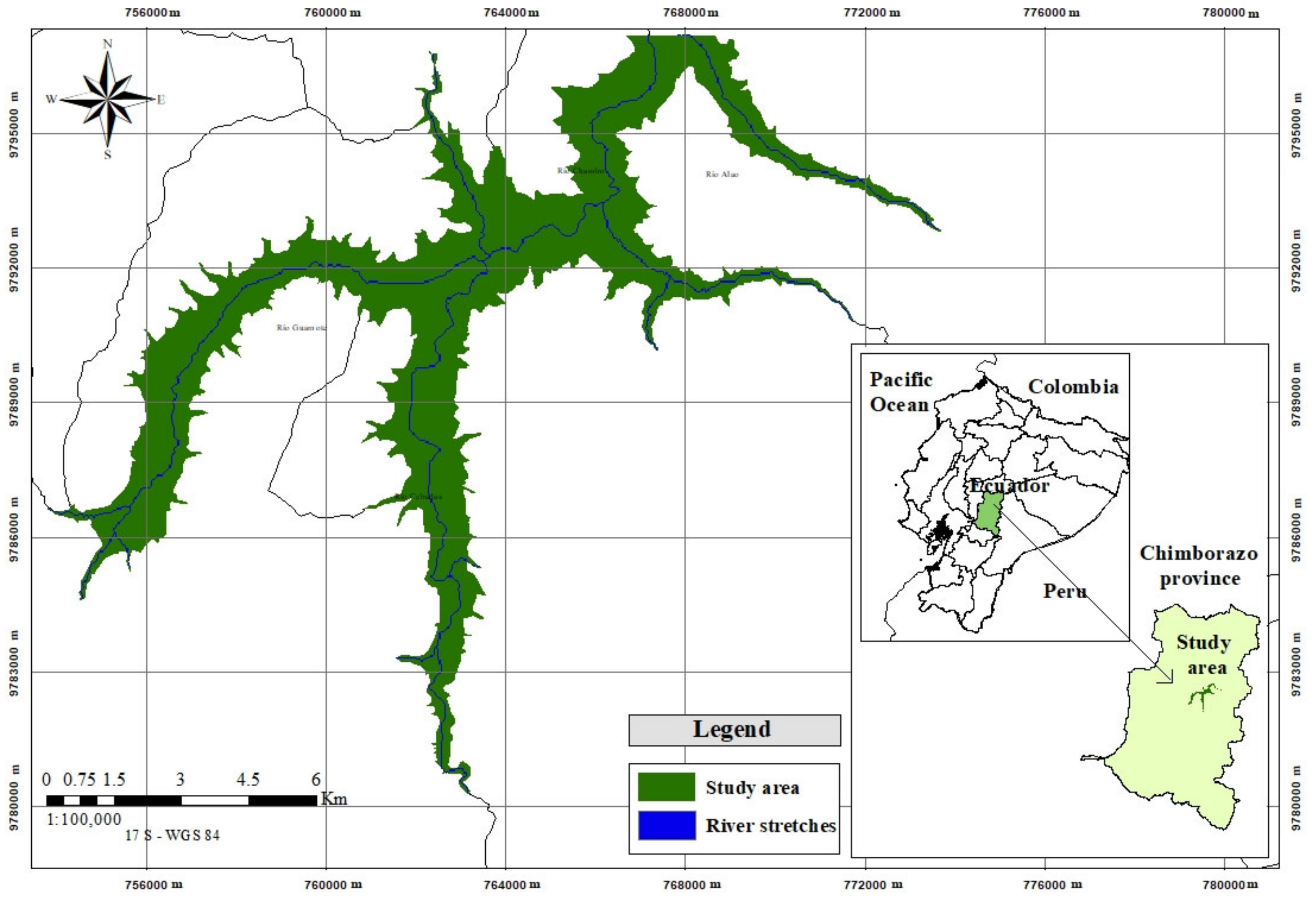
2.1. Study Area

The study area is situated in central Ecuador in the Interandean Valley or Depression (Figure 1) [46,47] within the Upper Middle Basin of the Chambo River between 2500 and 3000 m above sea level, which corresponds to sections of the main tributaries, being Guamote, Cebadas, and Alao.
For the first time, a water network formed by branches greater than and equal to three was identified, in order to distinguish the main tributaries within the Chambo River sub-basin. To accomplish this, using the GIS software, several steps were performed [48].
For the identification of the water network, we started with a tool that corrects the digital elevation model (DEM) raster by filling in the empty pixels, which was obtained from the U.S. Geological Survey Earth Explorer at 30 m resolution. Then, the direction information of flow from the DEM was obtained. In the same way, the accumulated flow for each cell was calculated [49]. Next, the flow accumulation raster was used in order to calculate the stream raster that indicates information from the drainage network. Subsequently, it was also converted into continuous segments to the drainage network using the raster of the drainage network and direction of flow. To create a raster of the order of the drainage based on the Strahler method [50], the raster generated with the previous tool was applied. In the last step, a drainage shapefile was generated from the order of the drainage and the flow direction, obtaining a shapefile of the water network. Analyses were conducted in ArcGIS.
For the delimitation of the hydrographic unit of the Chambo River, the contour lines and hydrography were obtained in the shapefile format from the Military Geographic Institute (IGM) web portal. Furthermore, the delimitation of the study area was realized through a stratification based on altitude ranges, where the area of interest was located in a range between 2500 and 3000 m above sea level using the corresponding DEM data, managing to determine a net area of 4669.42 hectares around the point of origin of the Chambo River. Thus, we obtained a fully defined area within the upper middle basin of the Chambo River. The focus of this investigation was the area associated with the study area; from this value, the control points of the investigation were determined using a completely random design and Fisher’s formula for the calculation of samples of finite populations [51], defining 355 control points.

2.2. Pre-Processing of Satellite Images

The Landsat 7, RapidEye, and Spot 6 satellite images were also used. The Landsat image was obtained from the United States Geological Survey Earth Explorer website, considering cloud cover less than 30% so that the visible field is as wide as possible, while the RapidEye and Spot images were provided by the PACHA project of the research group that supports the present study. The selection of the three types of satellite images was carried out in order to have the widest visible field possible in each of the years of study. The spatial resolution of the images was: 30 m for Landsat 7, 5 m for RapidEye, and 1–2 m for Spot 6.
The pre-processing was only applied to the Landsat image, since the RapidEye and Spot images were provided with the respective correction. The pre-processing of the Landsat 7 image implies an atmospheric correction, which requires a prior radiometric calibration that converts the digital number (ND) of each band into a radiance value (L), and to convert the radiance to reflectivity values in the top of atmosphere (TOA) [50]. In order to convert the ND values to radiance values, the radiometric rescaling factors G and B are used, which are specific for each band [52], and are supplied by the MTL metadata file. Subsequently, the calculated spectral radiance is converted into a planetary or exoatmospheric reflectance (TOA) [53]. In this way, the atmospheric correction is performed, using the dark subtraction method of the ENVI Software [54].

2.3. Classification Analyses

In the three satellite images used in this study, the combination of spectral bands in false-color was applied, that is, the three bands (blue, green and red) that correspond to the visible spectrum. This combination is the closest to the appreciation of the Earth with our eyes from space, in other words, a false color image is used to reveal or enhance features that would otherwise be invisible or poorly visible to the human eye [55]. In this phase, a supervised classification was conducted, in order to obtain a land cover map of the study area using the “Semi-Automatic Classification” library in the QGIS software. For this, it is necessary to establish control points, which refer to the areas or regions of interest (ROIs), also called training plots [56]. The 355 control points were identified in the field with the use of a GPS, a sample value that was calculated based on the study area hectares. The identification of these points was carried out randomly around the entire area, equally identifying the number of points in the five land cover classes. Later, they were located in the satellite images, adding the identified coverages with the “Macro Class List” tool, and then using the icon to create a polygon ROI [57].
For the methodology assignment phase, the maximum likelihood classifier was selected, also using the QGIS software, as it is a simple algorithm to apply and is considered as one of the most accurate and efficient discrimination procedures [58]. This algorithm produces the “spectral portrait” of each category based on the mean and variance of the training sites located in the satellite image. The data are considered to follow a normal distribution, which allows for working with a probability distribution model that allows each pixel to be assigned to the category with the highest probability of belonging [59]. On the other hand, the stratification of the study area consisted of identifying the present soil cover such as pasture, crops, soil and remnants of paramo, forest, and anthropic, which refers to constructions, roads, and any activity in which man intervenes, except the agricultural part that is already included in the other designated coverages.
The area delimited for the study is located in the upper middle basin of the Chambo River, where the upper zone corresponds to the Andean moorland and the lower zone to the productive part. The characteristic covers are pasture and Polylepis forests (paramo areas) [60], eucalyptus (Eucalyptus globulus), and pine (Pinus radiata) [61]. The latter is the main cause of changes in coverage, since they are introduced species that have the objective of increasing or diversifying the economic income of Andean peasants, reducing the erosion of degraded areas, and also as a carbon sequestration strategy [62]. Agricultural plots and anthropic constructions are coverages that have also been expanded due to the population increase.
The study area, located in the upper middle zone of the Chambo River basin, is composed only of the sections of the main rivers (Chambo, Guamote, Cebadas, and Alao) and their tributaries. The section of the Cebadas River (order 3) that was part of the study area is 17,148.14 m long and is delimited by the altitude of the 2880–3040 interval; the 16,163.84 m of the section of the Alao River (order 2) is delimited by 2760–3040; the section of the Guamote River (order 4) involved is 13,918 m located between 2840–3000; and the 9782.13 m section of the Chambo River (order 4) is located between 2760–2840. Then, the study area was stratified according to the types of coverage identified, considering the coverage of interest for the MAE, presented in its thematic legend, of levels I and II [63,64]:
-
Pasture (Level II): Vegetation characteristic of the slopes of the mountain ranges, belongs to the agricultural land group (Level I) of the coverage classification.
-
Crops (Level II): Coverage belonging to agricultural land. Annual, semi-permanent, and permanent crops can be identified in the Chambo River sub-basin, with corn and rice the predominant ones.
-
Forest: Coverage belonging to Level I of the coverage classification, which includes forest plantations and native forest (Level II). The forest cover present in this study area is composed of Polylepis forests (native), species of Eucalyptus globulus and Pinus radiata.
-
Anthropic Zone (Level I): Refers to the populated areas found in the sub-basin. Therefore, it refers to constructions and roads belonging to Level II of the aforementioned classification.
-
Soil and remnants of paramo: This refers to land with bare soil and remnants of vegetation belonging to paramo areas. They were not selected as separate covers because the existing density of paramo remnants is not significant.
The supervised classification was validated to analyze the land covers identified in the years 2000, 2009, and 2019 by applying an error matrix that allows for calculation of the precision measures and the Kappa index. The error matrix is a square matrix, and the rows and columns that make it up represent each of the categories of the land cover map obtained from the performed classification [65].
Within the precision measures, there is the Producer’s Accuracy (PA), which refers to the probability that a given class is correctly recognized, the User’s Accuracy (UA), which represents the probability that a pixel is correctly classified in the specific class to which it belongs, and the Overall Accuracy (OA), which indicates the proportion of the area correctly classified [66]. As for the Kappa index, it is a measure of the concordance between two maps considering all elements of the error matrix [67]. Consequently, the multi-temporal evaluation was directed to the identification of gains, losses, and persistence of each of the land covers. Therefore, a coverage change transitional matrix was used. This is a cross-tabulation matrix valued as an ideal tool for the descriptive analysis of transitions [66]. In this way, the changes and vulnerability measures were calculated, as listed in Table 1.
The cross tabulation matrix is also known as the change matrix in land use studies. It is composed of rows that have the information of the classes of time 1 and the columns of time 2 [67]. The parameters for the analysis of land cover changes determine the gains, losses, net change, total change, and exchanges for each class (cover) experienced between the two study times, and the total change is half of the sum of the changes in the individual categories. In the same way, it happens with the net change and the exchange, as the sum of the changes in the individual categories counts twice the change in the total area because the change in one cell of the matrix counts as a gain in one category and a loss in another category [68]. In addition, the Braimoh persistence indices relate the persistence of the loss and gain of each category [69].

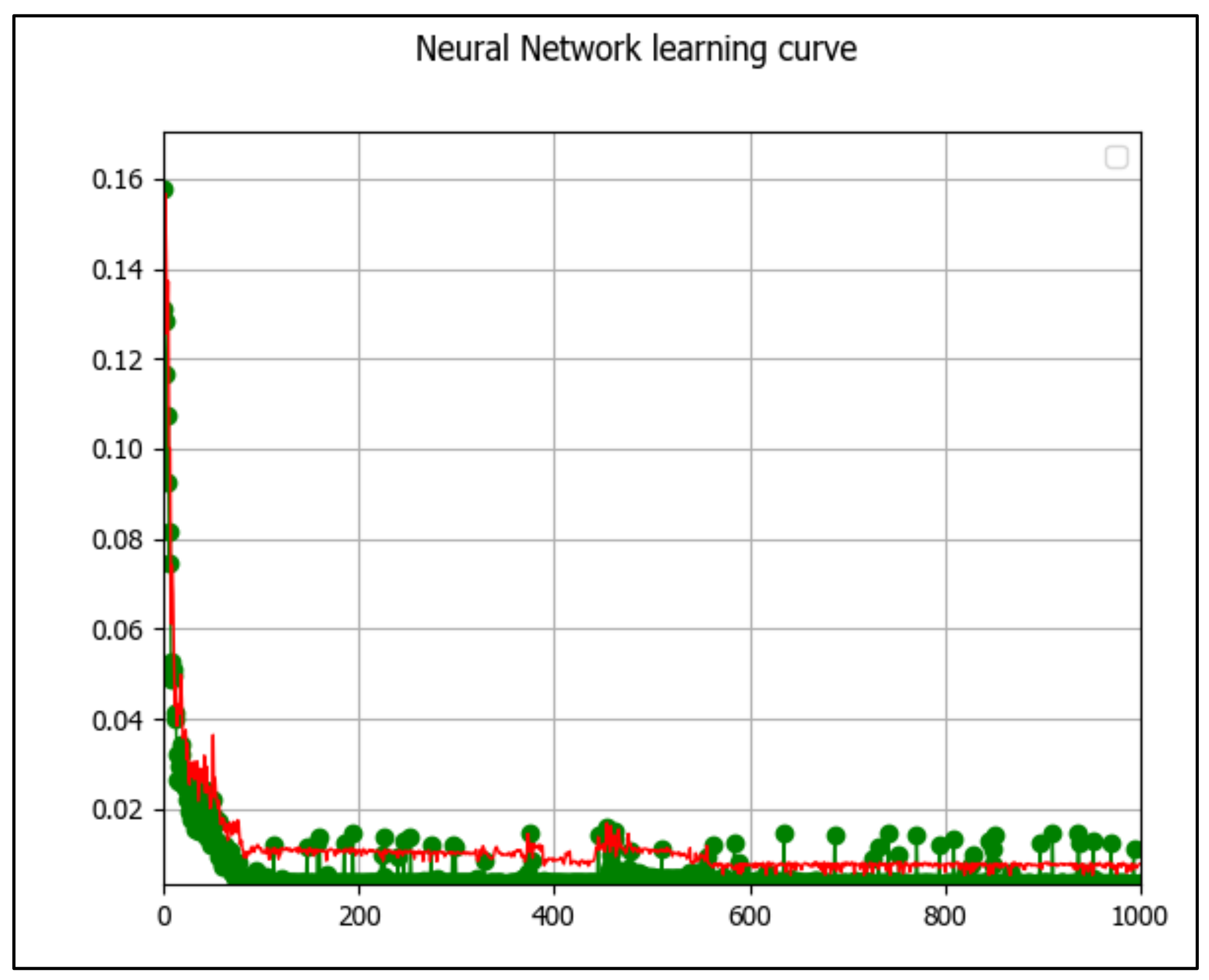
2.4. Projection to 2030

In order to generate the projection of the study area, the MOLUSCE complement of the QGIS software was applied, which, as its name indicates (Modules for Land Use Change Evaluation), refers to modules for the evaluation of changes in land use. This plugin has been designed to analyze, model, and simulate land use/cover changes effectively, where its graphical user interface has seven main submodules, allowing MOLUSCE to be valued as an intuitive and easy-to-use complement [70].
In order to obtain the cartographic projection for the year 2030 of the coverage present in the study area, the MOLUSCE methodology was applied with four submodules [70]. The first is the input, where the land cover maps (raster) of the last two years of study generated previously with the supervised classification are loaded. The second is the area changes, where the areas of each land cover are calculated, cover change transition matrices, and land cover maps. In the third, the transition potential modeling four modeling methods are available. These are artificial neural networks, weights of evidence, logistic regression and multicriteria evaluation. In the present study, we worked with the first method, where the learning algorithm examines the accuracy achieved in the sample sets (checkpoints) and training validations and also saves the best neural network in memory. The culmination of the training process occurs when the best precision is achieved [71]. The last submodule consisted of the simulation of cellular automata, which generates transition potential maps and the projection map (simulation) of the land cover (output).
A projection to 2030 will allow us to identify a possible scenario if the changes maintain the pattern of the last years studied. Sustainable development objectives were focused on this year, therefore, the associated projections contribute to decision-making to comply with the 2030 Agenda.

3. Results

3.1. Classification Analysis

The classification of satellite images allowed us to obtain coverage maps for each year of study (Figure 2). In 2000, it was evident that the predominant cover is that which corresponds to soil and the remnants of paramo with an area of 1563.17 ha (33.48%). Subsequently, there were crops, a coverage that has an area of 1186.07 ha (25.40%), followed by pasture cover with 928.39 ha (19.88%) and forest with an area of 875.45 ha (18.75%). The coverage with the smallest area referred to human activity, anthropic coverage, with 116.34 ha (2.49%).
For 2009, there was evidence of a change in the areas of each type of coverage. There, the predominant coverage is that of crops with 1868.52 ha (40.02), followed by pasture cover with an area of 1072.91 ha (22.98%), forest with 691.49 ha (14.81%), soil and paramo remnants with 713.23 ha. (15.27%), and, with the smallest area, the coverage of the anthropic zone with 323.28 ha (6.92%).
In 2019, the crop cover continued to be the predominant one with an area of 1791.43 ha (38.37%). Similarly, they were followed by pasture cover with 1211.71 ha (25.95%), forest with 813.04 ha (17.41%), soil and paramo remnants with 610.94 ha (13.08%), and the coverage corresponding to the anthropic zones had an area of 242.30 ha (5.19%).
To validate the supervised classification, the precision measures and the kappa index were calculated for each of the classifications in the three years of study. For this, an error matrix was generated for each year. The three coverage classification maps obtained from 2000 and 2009 presented acceptable global accuracy values, since they were in the range of 70–90% for the land cover classifications [72]. In addition, the accuracy of 2019 was 92.86%, considered as almost perfect (Table 2).
On the other hand, there is the value of the kappa index, which qualifies the force of concordance of the study values [73]. In this case, it is attributed to the concordance between the data taken in the field with those obtained from the classification performed by GIS software. The values corresponding to 2000 and 2009, which were 0.68 and 0.80 respectively, determine a considerable agreement of data, while the kappa index for the year 2019 indicated an almost perfect agreement, being a value of 0.91. Finally, the Table 3 presents the overall accuracy evaluation of this study.

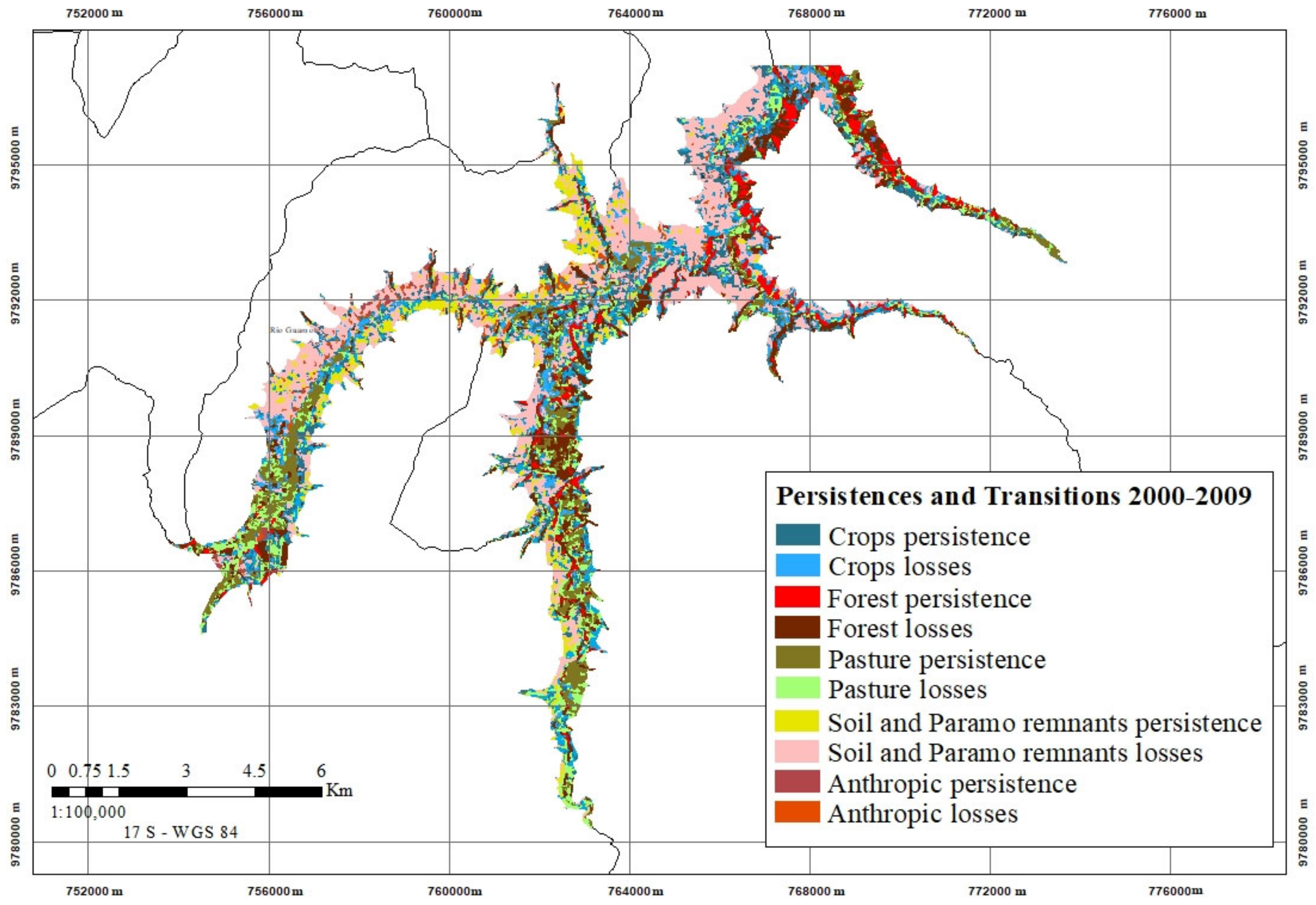
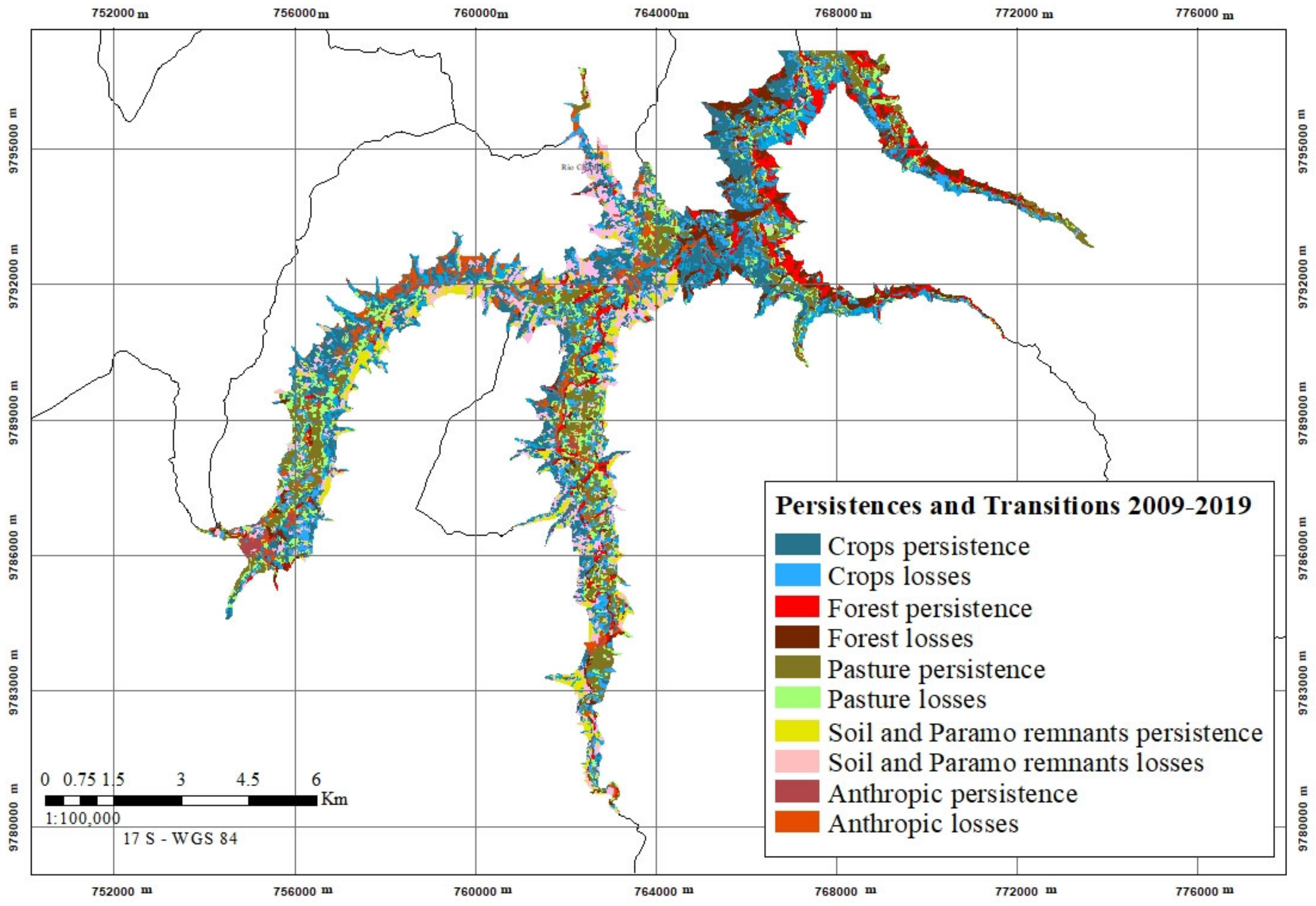
3.2. Change Trajectory Analysis

With the application of a cross-tabulation matrix, coverage transitions were identified, where the proportions of persistence of each category were located in the cells (blue) of the diagonal of the matrix, and the proportions corresponding to the categories that experienced transitions were found in the remaining cells (Table 4) [68]. Thus, the amount of landscape that did not experience any change in both intervals of time was cultivation, with 3871.6 ha until 2019.
In the time interval between 2000 and 2009, the transition with the greatest impact corresponded to the change in the soil and remnants from paramo to cultivation, with 17.39% of the total (green cell). These transitions are evident throughout the study area, but in greater quantity in the sections of the rivers located in the Cebadas and Pungalá parishes. Furthermore, in the period of 2009–2019, the transition with the greatest impact corresponded to that from crop to pasture with 8.06% of the total (green cell) (Table 5). These transitions are illustrated graphically in the cover persistence and transition map. Based on the values resolved in the previous point, it was possible to determine the rate of change in the two time periods of the investigation.
Table 6 lists the percentage values of the gains, losses, net change, exchange, and total change of the land covers analyzed in the study area. Between the years 2000 and 2009, the following values were identified such as a total change of 65.27%, a net change of 22.14%, and an exchange of 43.13%. The coverage corresponding to cultivation is the one that presented the most interactions with the other coverages, as it had an exchange value of 28.58%. In addition, the categories that registered area losses with respect to net change were forest with 3.94% and the soil and remnants of paramo with 18.20%. Hence, the land covers whose areas presented gains with respect to the net change were pasture with 3.10%, cultivation with 14.62%, and anthropic with 4.43%.
In the period 2009–2019, there was evidence of a total change of 51.04%, a net change of 5.58%, and an exchange of 45.47% of the study area (Table 7). The category that interacted in the highest percentage with the rest, as in the previous period, was that of cultivation, presenting a 34.58% exchange. In addition, the categories that register losses of area with respect to the net change were cultivation with 1.65%, anthropic with 1.73%, and the soil and remnants of paramo with 2.19%. On the other hand, the categories that registered gains in area with respect to the net change were pasture with 2.97% and forest with 2.60%.
In the first period of study (Figure 3), the cover corresponding to the soil and paramo remnants was the one that presented the highest percentage of loss (26.70%) in the first study period due to its transition to the other covers, as listed in Table 8. This value was three times (3.14) greater than the gain percentage (8.50%). In contrast, the class referring to crops was the one that showed the highest percentage of gain (28.91%), which corresponded to twice the percentage of losses (14.29%).
The forest category presented a loss percentage of 12.60%. As noted in the stratification of the study area, this category included forest plantations in general, and the native forests of the area. Continuing with the descending order of the loss percentages, there was the pasture category, which presented very close percentages of gains and losses at 13.19% and 10.09%, respectively.
In the time interval 2009–2019 (Figure 4), the category with the highest percentage of loss was cultivation with 18.94%. Despite this, this coverage practically lost what it gained. Next, there was the land cover and remnants of paramo, which significantly decreased its percentages of transitions compared to the period analyzed above. However, the tendency to present a higher percentage of loss (9.98%) than that of gain (7.79%) was maintained.
Regarding pasture cover, a higher percentage of gains (12.32%) than losses (9.35%) was observed, maintaining a trend similar to the previous period. In the forest category, in this period of time, it presented a higher percentage of the gains (10.48%) than the losses. The same occurred with anthropic coverage, quite the opposite of the previous period, where its percentage of losses (4.89%) was slightly higher than the percentage of gains (3.16%). The corresponding areas are presented in the Table 8 and Table 9.
Based on the coverage change analysis performed, the tables and maps that indicate the interactions recorded in this study are presented below (Figure 5 and Figure 6).
The persistence of the losses and gains were evaluated according to the tendency that the proportions in each category presented to decrease or increase. Table 10 lists the persistence coefficients of losses, gains, and net changes [69].
When the values of gp and lp are greater than 1, they indicate that there is a higher tendency to increase or decrease than to persistence [69]. In this way, in the period 2000–2009, all categories had a greater tendency to win than to persist, with the anthropic category being the one with the greatest impact (6.65). Similarly, this occurred with the tendency to lose, however, in this case, the most important value was the one belonging to the category soil and paramo remnants.
In the 2009–2019 period, except for the pasture and crop categories, all categories tended to win and lose more than to persist. Hereby, the coefficient corresponding to the anthropic class in the first period was a very high value compared to the others, even when compared to the value of the same class in the following period. Additionally, in those years, there was also a persistence of a loss of soil and paramo remnants.

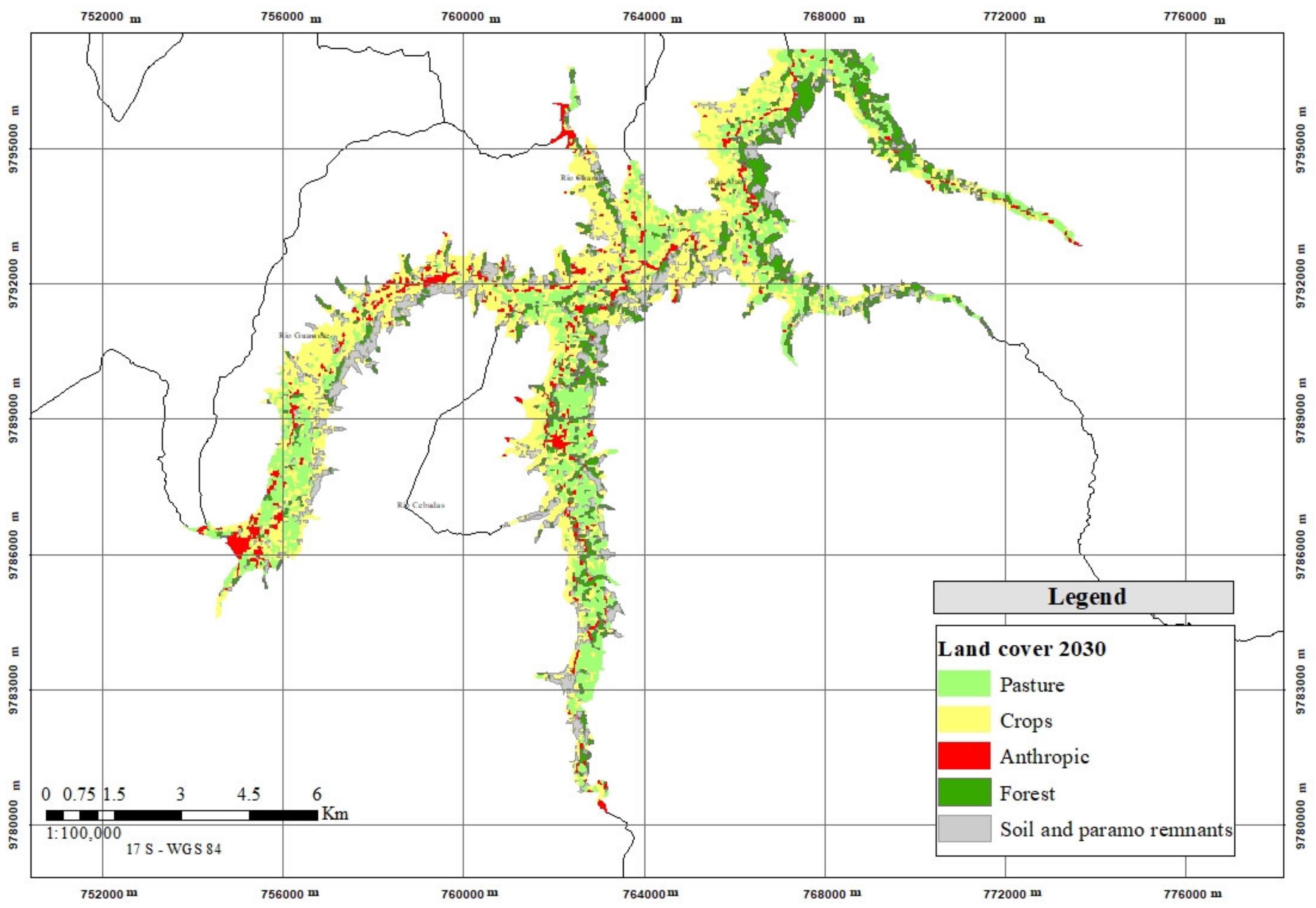
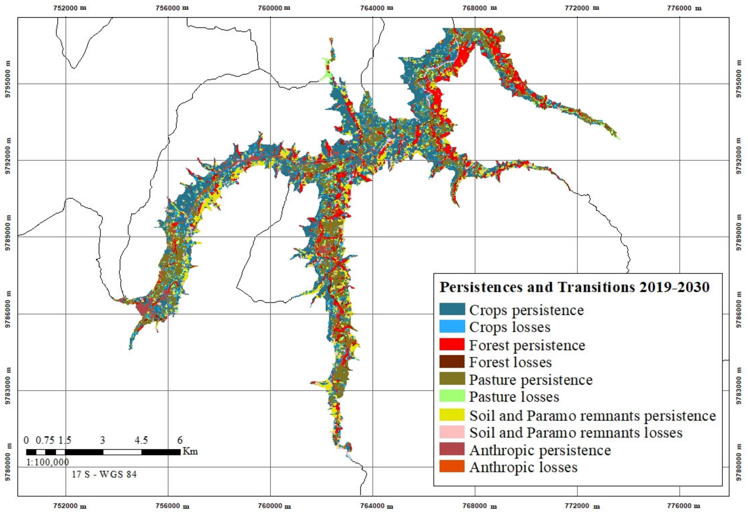
3.3. Cartographic Projection for the Year 2030

The projection for the year 2030 in the study area was obtained using the artificial neural network modeling method of the MOLUSCE complement. Where, in the first place, a neighborhood of nine pixels, a learning rate of 0.1, and a maximum of 1000 iterations were established [43], in order to obtain the neural network learning curve that was found, as illustrated in Figure 7, where the green color represents the training dataset and the red lines are from the validation dataset.
The general minimum validation error was 0.00527 and the current validation kappa was 97.33% for the simulation map of the land cover of the year 2030 (Figure 8).
Based on the simulation carried out, it is predicted that for the year 2030, the predominant cover will continue to be that of cultivation with an area of 1770.52 ha (37.92%), followed by pasture cover with 1191.72 ha (25.52%), forest with 757.53 ha (16.22%), and finally the soil and paramo remnants with 647.88 ha (13.87%) and the anthropic area with 301.77 ha (6.46%).
Table 11 presents a compilation of the values that determine the variation in the area of each of the categories in the period 2000–2019, based on previously obtained information. Additionally, the values belonging to the projection of the study area in the future (2030) are presented. Thus, based on the simulation carried out, it is predicted that between 2019 and 2030, there will be the following variations in each of the studied coverages (Figure 9):
The category that presents the highest percentage of variation will be anthropic, with a gain of 1.27%, followed by forest with an area loss of 1.19%, the soil and paramo remnants will present a gain of 0.79%, the crop cover will present a loss of 0.45%, and finally, the pasture cover will also present a decrease of 0.43% in its area.
Table 12 presents the prediction, for the year 2030, of the areas corresponding to the transitions and persistence of land cover.

4. Discussion

Landscape changes have been detected with greater emphasis from the 21st century, where each sector can present a different scenario. However, the increase in population, and therefore economic expansion, are the main factors of change in surface coverage [74], which have also been detected in the present study.
In the land cover classification of the time interval 2000–2009, it was detected that soil and paramo remnants had the highest area of loss, which can be attributable to the paramo degradation due to the fact that a large part of the paramos in the province of Chimborazo has been exposed to pressure through common practices of agriculture, livestock, and reforestation with introduced species. Furthermore, the burning of most of the straw is also a common practice, whose purpose is the regrowth of tender straw to feed cattle, thus increasing its productivity [75]. Despite, in the second period of study 2009–2019, the transitions having decreased, the pattern of the first period was maintained. Furthermore, this is mainly supported by the degradation of the paramos, which is linked to the gains of the other categories, because in addition to replacing the paramos, they also occupy the land without coverage (soil).
On the other hand, crops presented the highest gain of area. For this reason, it is appropriate to cite the Law of Agrarian Reform and Colonization, which entered into force in Ecuador in July 1964, proposing a new concept of obtaining land use rights. Therefore, up to 30 years after its application, the Ecuadorian Andes underwent a significant transformation, giving rise to the expansion of agricultural activities [76]. Nonetheless, regarding the loss of this cover, adding to the activities above-mentioned, the ash from volcanic eruptions has also been a problem that has contributed to the loss of crops [36,37].
In the case of the percentage of forest loss, the causes were also related to the causes of the categories described in the previous paragraphs, considering that the representative native forests of the study area were those located in the paramo zones. In the same way, colonization and agricultural expansion have caused the replacement of these forest covers. The profit value (8.66%) was supported by reforestation and afforestation activities, applied with different objectives such as the “Afforestation and reforestation project of the Chambo River sub-basin”, which sought to contribute to the environmental conditions in the sub-basin, using native species for protection and exotic for production. This completed project presented its results in 2008 [77].
The close percentages of gains and losses of pasture cannot represent a significant impact in the area in both periods of study. However, the floods in the sub-basin, especially in the middle part and in the part of the mouth, are presented as an important threat for this category, as it has been determined that along the Chambo River sub-basin, 28% of the areas affected by flooding correspond to planted pastures [78]. The greater gain than loss can be attributed to the afforestation and reforestation activities in previous years.
Regarding anthropic coverage, in the first interval of time, this class had a great tendency to win due to the typical population increase of societies. As the years went by, in the second period, their tendency to lose was greater than their tendency to win, a situation supported by the migration of the rural population to urban towns [36], considering that most of the study area corresponded to rural areas. Nevertheless, its percentage of loss was the one with the least impact compared to the other categories. Furthermore, according to the exchange rates calculated in the study periods, it is possible to determine that the future projection indicates the lowest values of coverage losses compared to previous years.
Comparing the results obtained, based on the measures of accuracy of the supervised classification, with Enderle and Weih [79], who developed a land cover classification of watersheds in Arkansas (USA) using supervised and unsupervised classification with images Landsat 7 (1995), in the present study, global accuracies between 75 and 93% were obtained, where the lowest accuracy being that corresponding to the Landsat 7 image of the year 2000, whose value was very close to that obtained in the supervised classification of the study in comparison. The same authors obtained a considerably lower global accuracy value of 40.94% in the unsupervised classification of the same image.
Similarly, Mohammady et al. [80] compared unsupervised and supervised land cover classification of a Baghsalian watershed in Iran with Landsat 7 images (2010), where their global accuracy values were between 58 and 78% in the first case and between 81 and 84% in the second case. In addition, the kappa index ranged between 0.57 and 0.74 and 0.79 and 0.82 as appropriate. Despite the fact that the supervised classification method was different to that in the present study, it was possible to determine that the supervised classification presented an appreciable advantage over the unsupervised classification of Landsat images, a situation repeated in other similar works such as in the case of Nijhawan et al. [81], who used the same method of the present investigation, and whose precision value was greater than that of the other types of classification.
The changes in coverage detected in this research are comparable with others performed in Ecuador such as in the Southern Andes [82], where their results agreed that the expansion of cultivable borders predominated over the rest of the coverage, in addition, the anthropic activity corresponding to the construction of roads and buildings was one of the most relevant causes of deforestation, without omitting its replacement by agricultural crops and pasture. According to Viña et al. [83] in their satellite evaluation of deforestation rates, carried out on the Colombia–Ecuador border between the years 1973 and 1996, they attributed the cause of deforestation to human colonization, a situation that is consistent with the results of this study of the first period (2000–2009), where the profit values of the anthropic zone were really high when compared with the rest of the coverages, and even in the second study period. Additionally, in an evaluation of changes in land use in the entire Chambo River basin between 1979 and 2014 [84], it was determined that one of the main transitions of coverage in that period was that of paramo to agricultural crops, a statement that agrees with the first study period in this work, where this transition was the one with the greatest area of change.
A further point is the projection made for the year 2030, where it would be expected that the area increase value of the anthropic zone would rise with respect to the first study period, where its value was representative. However, despite the fact that the projection estimated that there will be an increase, its value was not significant. At this point, we detected an uncertainty level in this MOLUSCE projection, because with the input of other variables such as a population growth rate between the years studied, the projected values can get even closer to a more accurate projection. This was corroborated by the study by Cosuegra et al. [85], which determined that migration from rural to urban areas in the different provinces of Ecuador has increased significantly since the 1970s due to the process of the development and growth of the main cities.
To complement this work, it would be important to perform a complementary study that relates spatial patterns with the water quality of the channels of the upper middle basin of the Chambo River, in order to link it with the impacts generated by changes in land cover. Similarly, these studies should involve an analysis of the effect of climate variability on the land use change and vice versa, and also on the livelihoods in the study area. This is to evaluate its impact on the change in coverage and determine the behavior of the population in the face of changes in coverage that have occurred over the years.

5. Conclusions

-
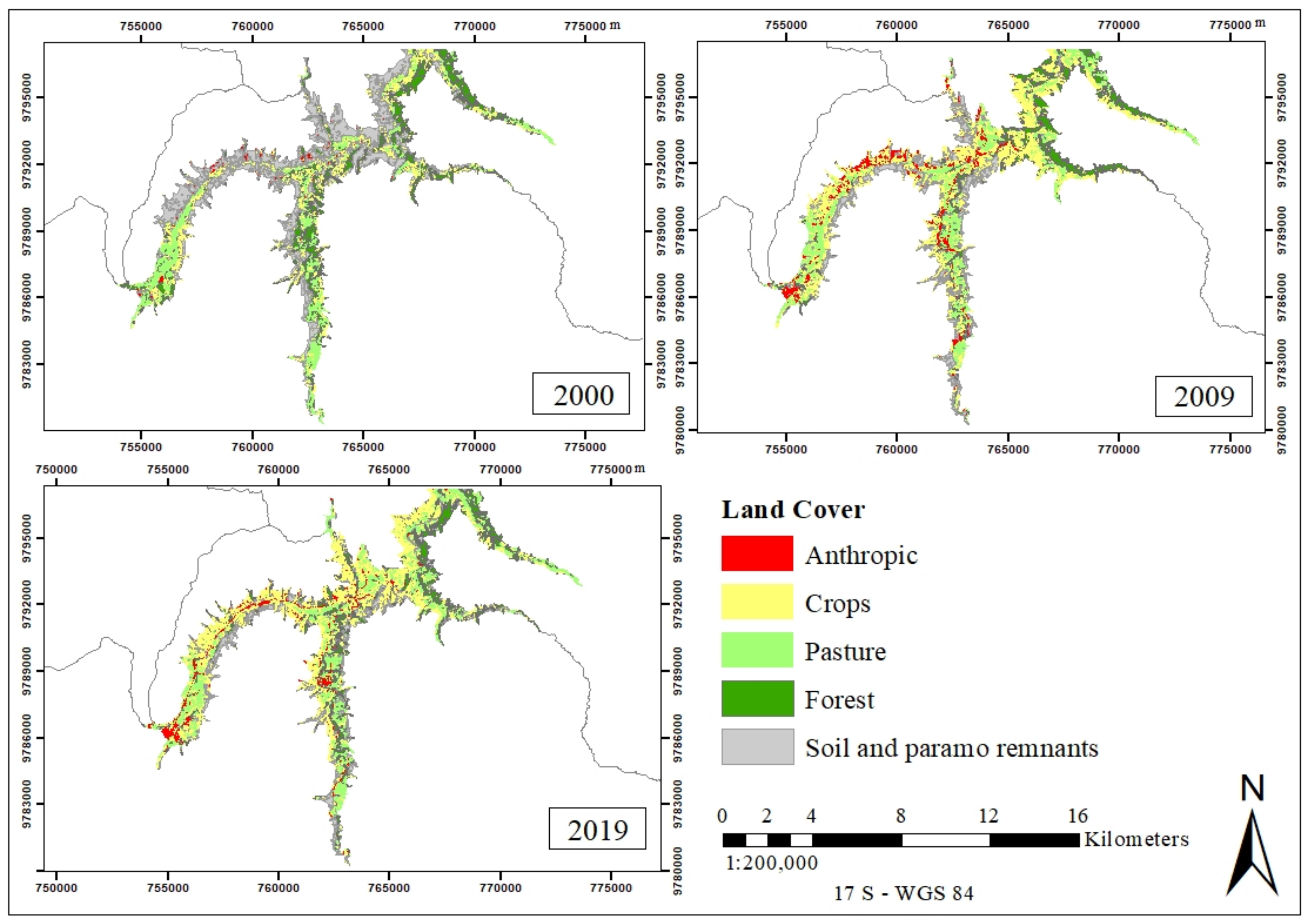
Through a supervised classification using the maximum likelihood algorithm, the study area located within the upper middle basin of the Chambo River sub-basin corresponding to its source area was stratified, where five predominant land covers were identified, being pasture, crops, soil-remnants of paramo, forest, and anthropic.
-
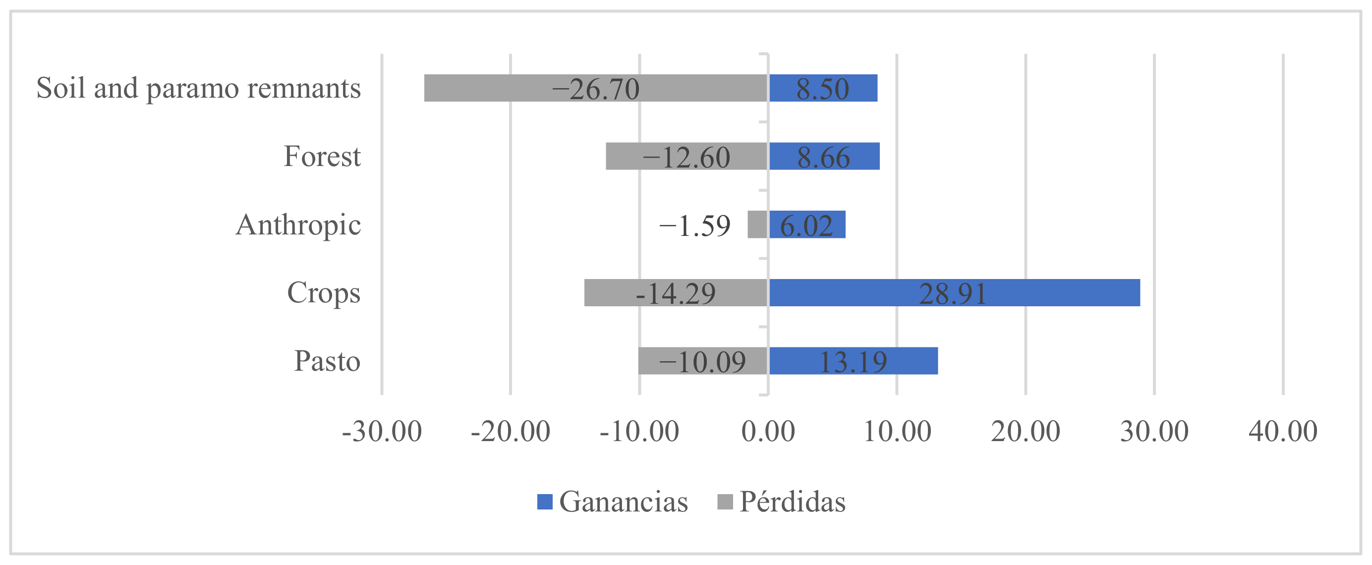
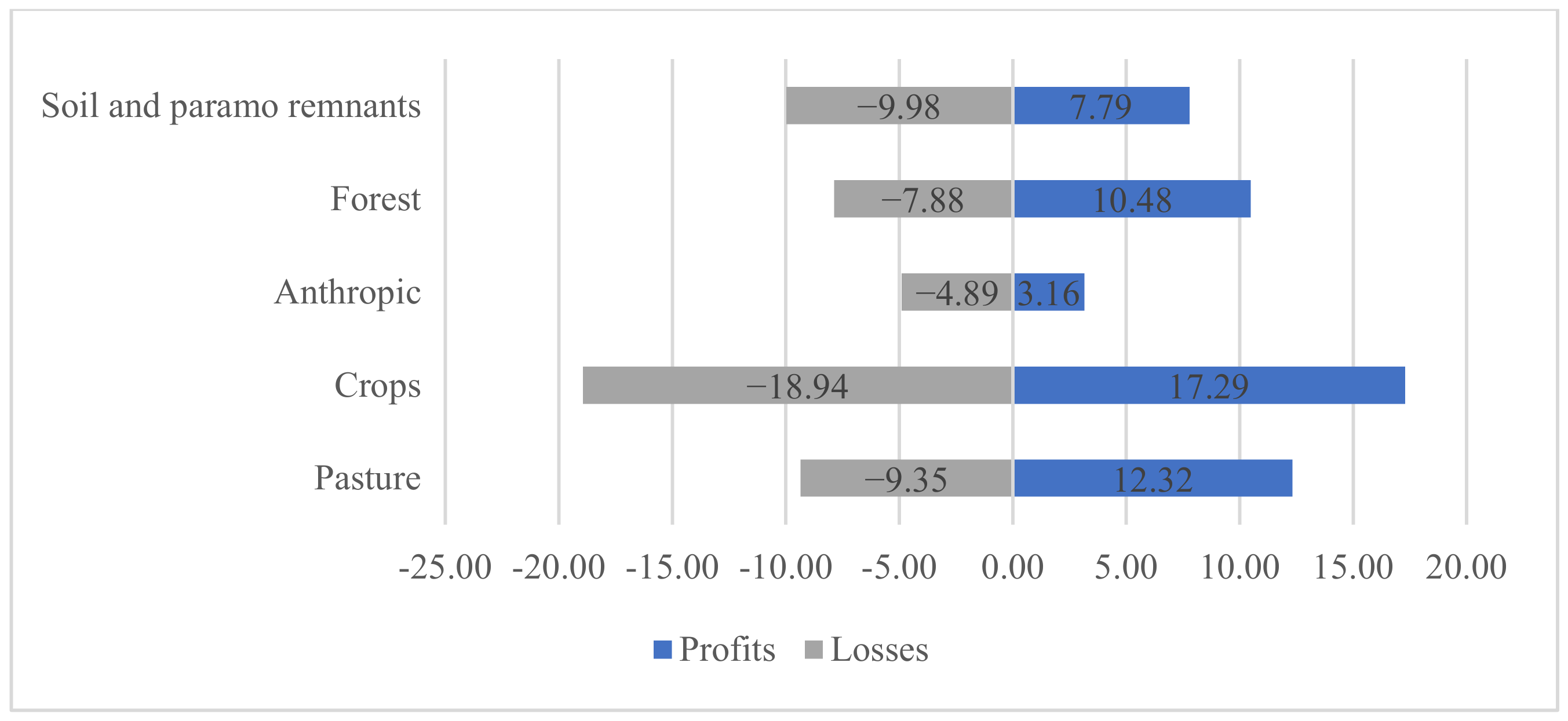
The obtained maps allowed us to identify that in the first period (2000–2009), the soil cover-paramo remnants presented the highest percentage of loss and the crop cover the highest percentage of gain, and in the second period (2009–2019), the crop presented the highest percentages of gains and losses, transitions were attributed to population growth, afforestation, reforestation, deforestation and agricultural activities, volcanic eruptions, land colonization, and the expansion of agricultural activity.
-
The cartographic projection of the coverage in the riparian ecosystem for the year 2030 allowed us to determine that the anthropic zone and soil-remnants of the paramo will increase their area and the areas of pasture, cultivation, and forest will be reduced as these percentages were insignificant and those with the least impact compared to the periods corresponding to previous years.

Author Contributions

Conceptualization, J.E.-P. and F.C.; methodology, J.E.-P. and F.C.; software, J.E.-P. and F.C.; validation, J.E.-P., F.C. and M.E.; formal analysis, J.E.-P.; investigation, J.E.-P. and T.T.; resources, M.E.; data curation, J.E.-P.; writing—original draft preparation, J.E.-P.; writing—review and editing, T.T.; visualization, J.E.-P. and T.T.; supervision, M.E.; project administration, M.E.; funding acquisition, J.E.-P., F.C., M.E. and T.T.; All authors have read and agreed to the published version of the manuscript.

Funding

This research received no external funding.

Conflicts of Interest

The authors declare no conflict of interest.

References

  1. Malanson, G.P. Riparian Landscapes; Cambridge Univ Press: Cambridge, UK, 1996. [Google Scholar]
  2. Sullivan, S.M.P.; Manning, D.W. Aquatic–terrestrial linkages as complex systems: Insights and advances from network models. Freshw. Sci. 2019, 38, 936–945. [Google Scholar] [CrossRef]
  3. Risser, P.G. The ecological importance of land-water ecotones. Ecol. Manag. Aquat. -Terr. Ecotones 1990, 4, 7–22. [Google Scholar]
  4. Krause, S.; Lewandowski, J.; Grimm, N.B.; Hannah, D.M.; Pinay, G.; McDonald, K.; Martí, E.; Argerich, A.; Pfister, L.; Klaus, J.; et al. Ecohydrological interfaces as hot spots of ecosystem processes. Water Resour. Res. 2017, 53, 6359–6376. [Google Scholar] [CrossRef] [Green Version]
  5. Naiman, R.J.; Decamps, H. The ecology of interfaces: Riparian zones. Annu. Rev. Ecol. Syst. 1997, 28, 621–658. [Google Scholar] [CrossRef] [Green Version]
  6. Stella, J.C.; Bendix, J. Multiple stressors in riparian ecosystems. In Multiple stressors in River Ecosystems; Elsevier: Amsterdam, The Netherlands, 2019; pp. 81–110. [Google Scholar]
  7. Gregory, S.V.; Swanson, F.J.; McKee, W.A.; Cummins, K.W. An ecosystem perspective of riparian zones. BioScience 1991, 41, 540–551. [Google Scholar] [CrossRef]
  8. Kutschker, A.; Brand, C.; Miserendino, M.L. Evaluación de La Calidad de Los Bosques de Ribera En Ríos Del NO Del Chubut Sometidos a Distintos Usos de La Tierra. Ecol. Austral 2009, 19, 19–34. Available online: https://www.researchgate.net/profile/Maria_Miserendino/publication/262141135_Evaluacion_de_la_calidad_de_los_bosques_de_ribera_en_rios_del_NO_del_Chubut_sometidos_a_distintos_usos_de_la_tierra/links/0deec536b8c3db01cf000000.pdf (accessed on 14 September 2020).
  9. Tonkin, J.D.; Merritt, D.; Olden, J.D.; Reynolds, L.V.; Lytle, D.A. Flow regime alteration degrades ecological networks in riparian ecosystems. Nat. Ecol. Evol. 2018, 2, 86–93. [Google Scholar] [CrossRef]
  10. Nilsson, C.; Berggren, K. Alterations of riparian ecosystems caused by river regulation: Dam operations have caused global-scale ecological changes in riparian ecosystems. How to protect river environments and human needs of rivers remains one of the most important questions of our time. BioScience 2000, 50, 783–792. [Google Scholar]
  11. Shafroth, P.B.; Stromberg, J.C.; Patten, D.T. Riparian vegetation response to altered disturbance and stress regimes. Ecol. Appl. 2002, 12, 107–123. [Google Scholar] [CrossRef]
  12. Talukdar, S.; Eibek, K.U.; Akhter, S.; Ziaul, S.K.; Islam, A.R.M.T.; Mallick, J. Modeling Fragmentation Probability of Land-Use and Land-Cover Using the Bagging, Random Forest and Random Subspace in the Teesta River Basin, Bangladesh. Ecol. Indic. 2021, 126, 107612. [Google Scholar] [CrossRef]
  13. Zhou, P.; Luukkanen, O.; Tokola, T.; Nieminen, J. Effect of vegetation cover on soil erosion in a mountainous watershed. Catena 2008, 75, 319–325. [Google Scholar] [CrossRef]
  14. Sánchez, V.D.R.S.; Tafur, J.R.A.; De la Vera, K.R.; Sánchez, M.S.A.; Alulema, A.C.L.; Ponce, L.R.A.; Morales, J.L.P.; Benavides, M.J.Z.; Pozo, M.D.R.; Campoverde, J.A.Y.; et al. Use of Geotechnologies and Multicriteria Evaluation in Land Use Policy-The Case of the Urban Area Expansion of the City of Babahoyo, Ecuador. In Proceedings of the 2019 Sixth International Conference on eDemocracy & eGovernment (ICEDEG), Quito, Ecuador, 24–26 April 2019; IEEE: Piscataway, NJ, USA, 2019; pp. 194–202. [Google Scholar]
  15. Barreto-Álvarez, D.E.; Heredia-Rengifo, M.G.; Padilla-Almeida, O.; Toulkeridis, T. Multitemporal evaluation of the recent land use change in Santa Cruz Island, Galapagos, Ecuador. In Information and Communication Technologies, Proceedings of the 8th Conference, TICEC 2020, Guayaquil, Ecuador, 25–27 November 2020; Springer: Cham, Switzerland, 2020; pp. 519–534. [Google Scholar]
  16. Heredia-R, M.; Cayambe, J.; Schorsch, C.; Toulkeridis, T.; Barreto, D.; Poma, P.; Villegas, G. Multitemporal Analysis as a Non-Invasive Technology Indicates a Rapid Change in Land Use in the Amazon: The Case of the ITT Oil Block. Environments 2021, 8, 139. [Google Scholar] [CrossRef]
  17. Pabón, J.D.; Rodríguez, N.; Bernal, N.R.; Castiblanco, M.A.; Sánchez, Y.V. Modelamiento Del Efecto Del Cambio En El Uso Del Suelo En El Clima Local-Regional Sobre Los Andes Colombianos. Rev. De Acad. Colomb. De Cienc. Exactas Físicas Y Nat. 2014, 37, 380–381. [Google Scholar] [CrossRef]
  18. Bronstert, A.; Niehoff, D.; Bürger, G. Effects of climate and land-use change on storm runoff generation: Present knowledge and modelling capabilities. Hydrol. Process. 2002, 16, 509–529. [Google Scholar] [CrossRef]
  19. Saad, R.; Koellner, T.; Margni, M. Land use impacts on freshwater regulation, erosion regulation, and water purification: A spatial approach for a global scale level. Int. J. Life Cycle Assess. 2013, 18, 1253–1264. [Google Scholar] [CrossRef]
  20. Alvarado, D. Dinámica Espacio-Temporal de La Cobertura de Bosque Seco Tropical Del Departamento Del Valle Del Cauca, Colombia. 2014, pp. 5–15. Available online: https://www.researchgate.net/publication/267626550_Dinamica_Espacio-Temporal_de_la_cobertura_de_Bosque_Seco_Tropical_del_Departamento_del_Valle_del_Cauca_Colombia (accessed on 13 September 2020).
  21. Toulkeridis, T.; Tamayo, E.; Simón-Baile, D.; Merizalde-Mora, M.J.; Reyes–Yunga, D.F.; Viera-Torres, M.; Heredia, M. Climate Change according to Ecuadorian academics–Perceptions versus facts. LA GRANJA. Rev. Cienc. Vida 2020, 31, 21–46. [Google Scholar] [CrossRef] [Green Version]
  22. Karamesouti, M.; Detsis, V.; Kounalaki, A.; Vasiliou, P.; Salvati, L.; Kosmas, C. Land-use and land degradation processes affecting soil resources: Evidence from a traditional Mediterranean cropland (Greece). Catena 2015, 132, 45–55. [Google Scholar] [CrossRef]
  23. Teketay, D. Deforestation, wood famine, and environmental degradation in Ethiopia’s highland ecosystems: Urgent need for action. Northeast. Afr. Stud. 2001, 8, 53–76. [Google Scholar] [CrossRef]
  24. Abid, M.; Schilling, J.; Scheffran, J.; Zulfiqar, F. Climate change vulnerability, adaptation and risk perceptions at farm level in Punjab, Pakistan. Sci. Total Environ. 2016, 547, 447–460. [Google Scholar] [CrossRef]
  25. Triplett, G.B., Jr.; Dick, W.A. No-tillage crop production: A revolution in agriculture! Agron. J. 2008, 100, S-153. [Google Scholar] [CrossRef]
  26. Scolozzi, R.; Geneletti, D. A Multi-Scale Qualitative Approach to Assess the Impact of Urbanization on Natural Habitats and Their Connectivity. Environ. Impact Assess. Rev. 2012, 36, 9–22. [Google Scholar] [CrossRef]
  27. Fischer, J.; Lindenmayer, D.B. Landscape modification and habitat fragmentation: A synthesis. Glob. Ecol. Biogeogr. 2007, 16, 265–280. [Google Scholar] [CrossRef]
  28. Pardini, R.; Nichols, E.; Püttker, T. Biodiversity response to habitat loss and fragmentation. Encycl. Anthr. 2017, 3, 229–239. [Google Scholar]
  29. Hobbs, R.J. Effects of landscape fragmentation on ecosystem processes in the Western Australian wheatbelt. Biol. Conserv. 1993, 64, 193–201. [Google Scholar] [CrossRef]
  30. Suarez, A.V.; Bolger, D.T.; Case, T.J. Effects of fragmentation and invasion on native ant communities in coastal southern California. Ecology 1998, 79, 2041–2056. [Google Scholar] [CrossRef]
  31. Farnum, F.; Vielka, M. Análisis Multitemporal (1970–2017) Del Uso Del Suelo en Cinco Comunidades Ubicadas a lo Largo de la Carretera Boydroosevelt, Panamá. 2019, pp. 108–110. Available online: https://www.researchgate.net/publication/334283429_ANALISIS_MULTITEMPORAL_1970-2017_DEL_USO_DEL_SUELO_EN_CINCO_COMUNIDADES_UBICADAS_A_LO_LARGO_DE_LA_CARRETERA_BOYDROOSEVELT_PANAMA (accessed on 13 September 2020).
  32. Chuvieco, E. Teledeteccion Ambiental—Emilio Chuvieco Salinero. 1995. Available online: https://books.google.es/books?id=aKsNXCVCtcQC&printsec=frontcover&dq=teledeteccion+ambiental&hl=es&sa=X&ved=0ahUKEwiE6vLagfbOAhULkRQKHQg2AhMQ6AEIGzAA#v=onepage&q=teledeteccionambiental&f=false (accessed on 13 September 2020).
  33. Massonne, H.J.; Toulkeridis, T. Widespread relics of high-pressure metamorphism confirm major terrane accretion in Ecuador: A new example from the Northern Andes. Int. Geol. Rev. 2012, 54, 67–80. [Google Scholar] [CrossRef]
  34. Toulkeridis, T.; Chunga, K.; Rentería, W.; Rodriguez, F.; Mato, F.; Nikolaou, S.; Cruz D’Howitt, M.; Besenzon, D.; Ruiz, H.; Parra, H.; et al. The 7.8 Mw Earthquake and Tsunami of the 16th April 2016 in Ecuador—Seismic evaluation, geological field survey and economic implications. Sci. Tsunami Hazards 2017, 36, 197–242. [Google Scholar]
  35. Chidichimo, F.; Mendoza, B.T.; De Biase, M.; Catelan, P.; Straface, S.; Di Gregorio, S. Hydrogeological modeling of the groundwater recharge feeding the Chambo aquifer, Ecuador. In AIP Conference Proceedings; AIP Publishing LLC: Melville, NY, USA, 2018; Volume 2022, p. 020003. [Google Scholar]
  36. PDOT-Chambo. ACTUALIZACIÓN DEL PLAN DE DESARROLLO Y ORDENAMIENTO TERRITORIAL DEL CANTÓN CHAMBO. 2019; pp. 52–2014. Available online: https://app.sni.gob.ec/sni-link/sni/PORTAL_SNI/data_sigad_plus/sigadplusdiagnostico/0660001680001_DIAGNOSTICO%20PDyOT%20CHAMBO%202014-2019_15-01-2015_16-16-38.pdf (accessed on 15 September 2020).
  37. Toulkeridis, T.; Zach, I. Wind directions of volcanic ash-charged clouds in Ecuador–implications for the public and flight safety. Geomat. Nat. Hazards Risk 2017, 8, 242–256. [Google Scholar] [CrossRef] [Green Version]
  38. Toulkeridis, T.; Arroyo, C.R.; Cruz D’Howitt, M.; Debut, A.; Vaca, A.V.; Cumbal, L.; Mato, F.; Aguilera, E. Evaluation of the initial stage of the reactivated Cotopaxi volcano–analysis of the first ejected fine-grained material. Nat. Hazards Earth Syst. Sci. Discuss. 2015, 3, 6947–6976. [Google Scholar]
  39. Toulkeridis, T.; Seqqat, R.; Arias, M.T.; Salazar-Martinez, R.; Ortiz-Prado, E.; Chunga, S.; Vizuete, K.; Heredia-R, M.; Debut, A. Volcanic Ash as a precursor for SARS-CoV-2 infection among susceptible populations in Ecuador: A satellite Imaging and excess mortality-based analysis. In Disaster Medicine and Public Health Preparedness; Cambridge University Press: Cambridge, UK, 2021; pp. 1–13. [Google Scholar]
  40. MAGAP; MAE. Mapa de Cobertura y Uso de La Tierra Del Ecuador Continental 2013–2014. 2015. Available online: https://app.sni.gob.ec/sni-link/sni/Portal%20SNI%202014/USO%20DE%20LA%20TIERRA/05-MAPA_NACIONAL_COBERTURA_USO.pdf (accessed on 20 September 2020).
  41. MAE (Ministerio del Ambiente Ecuador). Evaluación de Necesidades Tecnológicas Para El Manejo de La Oferta Hídrica En Cantidad y Calidad. 2013. Available online: https://tech-action.unepdtu.org/wp-content/uploads/sites/2/2013/12/evaluacionnecesidadestecnologicas-adaptacion-ofertahidrica-ecuador-12.pdf (accessed on 20 September 2020).
  42. Ochoa-Tocachi, B.F.; Buytaert, W.; De Bievre, B.; Célleri, R.; Crespo, P.; Villacís, M.; Llerena, C.A.; Acosta, L.; Villazón, M.; Guallpa, M.; et al. Impacts of Land Use on the Hydrological Response of Tropical Andean Catchments. Hydrol. Process. 2016, 30, 4074–4089. [Google Scholar] [CrossRef] [Green Version]
  43. Suárez, G.; Olaya, L. Aplicación de Un Modelo Predictivo Para El Análisis Del Impacto Generado Por El Cambio de Cobertura Urbana En El Municipio de Mosquera, Cundinamarca; Universidad Distrital Francisco José de Caldas: Bogotá, Colombia, 2018. [Google Scholar]
  44. Clerici, N.; Paracchini, M.L.; Maes, J. Land-Cover Change Dynamics and Insights into Ecosystem Services in European Stream Riparian Zones. Ecohydrol. Hydrobiol. 2014, 14, 107–120. [Google Scholar] [CrossRef]
  45. Pazmiño, Y.; de Felipe, J.J.; Vallbé, M.; Cargua, F.; Quevedo, L. Identification of a Set of Variables for the Classification of Páramo Soils Using a Nonparametric Model, Remote Sensing, and Organic Carbon. Sustainability 2021, 13, 9462. [Google Scholar] [CrossRef]
  46. Fiorini, E.; Tibaldi, A. Quaternary tectonics in the central Interandean Valley, Ecuador: Fault-propagation folds, transfer faults and the Cotopaxi Volcano. Glob. Planet. Chang. 2012, 90, 87–103. [Google Scholar] [CrossRef]
  47. Winkler, W.; Villagómez, D.; Spikings, R.; Abegglen, P.; Egüez, A. The Chota basin and its significance for the inception and tectonic setting of the inter-Andean depression in Ecuador. J. South Am. Earth Sci. 2005, 19, 5–19. [Google Scholar] [CrossRef]
  48. Jumbo, F. Delimitación Automática de Microcuencas Utilizando Datos SRTM de La NASA (Automatic Delimitation of Microwatershed Using SRTM Data of the NASA). Enfoque UTE 2015, 6, 81–97. Available online: https://ingenieria.ute.edu.ec/enfoqueute/ (accessed on 20 September 2020). [CrossRef] [Green Version]
  49. Zhica, J. Caracterización Morfométrica y Estudio Hidrológico de La Microcuenca Del Río San Francisco, Cantón; Universidad Politécnica Salesiana: Cuenca, Ecuador, 2020. [Google Scholar]
  50. Vega, X. Diferentes Soluciones Para La Delimitación y Codificación de Cuencas Superficiales Cubanas. Ing. Hidráulica Ambient. 2020, 41, 75–84. [Google Scholar]
  51. Aguilar, S. Fórmulas Para El Cálculo de La Muestra En Investigaciones de Salud. Salud Tabasco 2005, 11, 333–338. Available online: https://www.redalyc.org/articulo.oa?id=48711206 (accessed on 20 September 2020).
  52. Arias, H.A.; Zamora, R.M.; Bolaños, C.V. Metodología Para La Corrección Atmosférica de Imágenes ASTER, RAPIDEYE, SPOT 2 Y LANDSAT 8 Con El Módulo FLAASH Del Software ENVI. Rev. Geográfica América Cent. 2014, 2, 39–59. Available online: https://www.redalyc.org/pdf/4517/451744544002.pdf (accessed on 25 September 2020).
  53. Chander, G.; Markham, B. Revised Landsat-5 TM Radiometrie Calibration Procedures and Postcalibration Dynamic Ranges. IEEE Trans. Geosci. Remote Sens. 2003, 41, 2674–2677. [Google Scholar] [CrossRef]
  54. Wilson, C.O.; Weng, Q. Simulating the Impacts of Future Land Use and Climate Changes on Surface Water Quality in the Des Plaines River Watershed, Chicago Metropolitan Statistical Area, Illinois. Sci. Total Environ. 2011, 409, 4387–4405. [Google Scholar] [CrossRef]
  55. Fernández, I.; Herrero, E. El Satélite Landsat. Análisis Visual de Imágenes Obtenidas Del Sensor ETM+ Satélite Landsat. 2001. Available online: https://www.cartesia.org/data/apuntes/teledeteccion/landsat-analisis-visual.pdf (accessed on 25 September 2020).
  56. Paegelow, M.; Camacho Olmedo, M.T. Modelos de Simulacion Espacio-Temporal y Teledeteccion: El Método de La Segmentacion Para La Cartografia Cronologica de Usos Del Suelo. 2010. Available online: https://halshs.archives-ouvertes.fr/halshs-01063980 (accessed on 30 September 2020).
  57. Brenes, C. Tutorial de Clasificación Supervisada de Imágenes de Satétite Con QGIS y R Statistics; Managua, Nicaragua, 2019. [Google Scholar] [CrossRef]
  58. Maselli, F.; Conese, C.; De Filippis, T.; Romani, M. Integration of Ancillary Data into a Maximum-Likelihood Classifier with Nonparametric Priors. ISPRS J. Photogramm. Remote Sens. 1995, 50, 2–11. [Google Scholar] [CrossRef]
  59. García Mora, T.J.; Mas, J.F. Comparación de Metodologías Para El Mapeo de La Cobertura y Uso Del Suelo En El Sureste de México Comparison of Methodologies for Mapping Land Use Cover in Southeast Mexico. Investig. Geográficas 2008, 67, 7–19. [Google Scholar]
  60. Gismondi, M.; Kamusoko, C.; Furuya, T.; Tomimura, S.; Maya, M. MOLUSCE An Open Source Land Use Change Analyst for QGIS. 2014. Available online: https://www.ajiko.co.jp/download/pdf_tf2014/p62-63.pdf (accessed on 30 September 2020).
  61. Palacios, J. Evaluación de La Dinámica Del Cambio de La Cobertura y Uso de Tierra En El Área de Influencia de La Propuesta de Carretera Bellavista, Mazan, Salvador, El Estrecho. 2019. Available online: https://terra.iiap.gob.pe/assets/files/riesgos/2018/01_2018_EVALUACION_DINAMICA_CAMBIO_DE_COBERTURA_ESTRECHO.pdf (accessed on 30 September 2020).
  62. Bautista, K. Estudio Del Aprovechamiento Hídrico de La Microcuenca Del Río Alao Desde Los Usos de Concesión. Esc. Super. Politécnica Chimborazo 2009, 2, 3500. [Google Scholar]
  63. Bautista Rojas, V.I. Estudio de La Calidad Del Agua de La Cuencas Del Rio Chambo En Época de Estiaje. Escuela Superior Politécnica de Chimborazo, vol. Bachelor. 2014. Available online: https://dspace.espoch.edu.ec/handle/123456789/3221 (accessed on 30 September 2020).
  64. Echeverría, J. Dinámica Espacial de La Cobertura de Ribera de La Zona de Influencia Del Río Chambo; Escuela Superior Politécnica de Chimborazo: Riobamba, Ecuador, 2021; Available online: http://dspace.espoch.edu.ec/handle/123456789/15313#:~:text=La%20proyecci%C3%B3n%20cartogr%C3%A1fica%20de%20la,disminuir%C3%A1n%20en%200.45%25%20y%200.43%25 (accessed on 30 September 2020).
  65. Anupam, A. Accuracy Assesment. Ignou: The people´s University. 2017. Available online: https://www.researchgate.net/publication/324943246_UNIT_14_ACCURACY_ASSESSMENT (accessed on 30 September 2020).
  66. Ayala-Izurieta, J.E.; Márquez, C.O.; García, V.J.; Recalde-Moreno, C.G.; Rodríguez-Llerena, M.V.; Damián-Carrión, D.A. Land Cover Classification in an Ecuadorian Mountain Geosystem Using a Random Forest Classifier, Spectral Vegetation Indices, and Ancillary Geographic Data. Geosciences 2017, 7, 34. [Google Scholar] [CrossRef] [Green Version]
  67. Plata, W. Descripción, Análisis y Simulación Del Crecimiento Urbano Mediante Tecnologías de La Información Geográfica. El Caso de La Comunidad de Madrid. Universidad de Alcalá. 2010. Available online: https://dialnet.unirioja.es/servlet/tesis?codigo=89948&info=resumen&idioma=ENG (accessed on 30 September 2020).
  68. Pontius, R.G., Jr.; Shusas, E.; McEachern, M. Detecting Important Categorical Land Changes While Accounting for Persistence. Agric. Ecosyst. Environ. 2004, 101, 251–268. [Google Scholar] [CrossRef]
  69. Braimoh, A. Random and Systematic Land-Cover Transitions in Northern Ghana. Agric. Ecosyst. Environ. 2006, 113, 254–263. [Google Scholar] [CrossRef]
  70. Vargas, O.; Patricia, V. Páramos Andinos Reviviendo Nuestros Páram Os Restauración Ecológica de Páramos. Proyecto Páramo Andino. 2011. Available online: https://biblio.flacsoandes.edu.ec/libros/digital/56494.pdf (accessed on 30 September 2020).
  71. MAE; MAGAP. Protocolo Metodológico Para La Elaboración Del Mapa de Cobertura y Uso de La Tierra Del Ecuador Continental 2013–2014, Escala 1:100.000. May 2013. Available online: www.magap.gob.ec (accessed on 30 September 2020).
  72. Li, Y.; Zhu, X.; Pan, Y.; Gu, J.; Zhao, A.; Liu, X. A Comparison of Model-Assisted Estimators to Infer Land Cover/Use Class Area Using Satellite Imagery. Remote Sens. 2014, 6, 8904–8922. [Google Scholar] [CrossRef] [Green Version]
  73. Landis, J.R.; Koch, G.G. The Measurement of Observer Agreement for Categorical Data. Biometrics 1977, 33, 159. [Google Scholar] [CrossRef] [Green Version]
  74. Muhammad, R.; Zhang, W.; Abbas, Z.; Guo, F.; Gwiazdzinski, L. Spatiotemporal Change Analysis and Prediction of Future Land Use and Land Cover Changes Using QGIS MOLUSCE Plugin and Remote Sensing Big Data: A Case Study of Linyi, China. Land 2022, 11, 419. [Google Scholar] [CrossRef]
  75. Bustamante, M.; Alban, M.; Arguello, M. Los Páramos de Chimborazo. Un Estudio Socioambiental Para La Toma de Decisiones. EcoCiencia & CONDENSAN. 2011. Available online: https://biblio.flacsoandes.edu.ec/libros/digital/56619.pdf (accessed on 1 November 2020).
  76. Pierre, H. 30 Años de Reforma Agraria y Colonización En El Ecuador: 1964-1994; Dinámicas Espaciales: Quito, Ecuador, 2001. [Google Scholar]
  77. FIEDS. Proyecto Forestación y Reforestación de La Subcuenca Del Río Chambo|Fieds.Org. 2017. Available online: https://fieds.org/historia-fie/convocatoria/proyecto-forestacion-y-reforestacion-de-la-subcuenca-del-rio-chambo/ (accessed on 1 November 2020).
  78. Arias, H.; Miguel, P. Estudio Hidráulico Del Río Chambo Para La Determinación de La Conductancia Entre Río-Acuífero y Zonas de Inundación. Universidad Nacional de Chimborazo, 2018. 2018. Available online: https://dspace.unach.edu.ec/handle/51000/4876 (accessed on 3 November 2020).
  79. Enderle, D.I.; Weih, R.C., Jr. Integrating Supervised and Unsupervised Classification Methods to Develop a More Accurate Land Cover Classification. J. Ark. Acad. Sci. 2005, 59, 65–73. Available online: https://scholarworks.uark.edu/jaas/vol59/iss1/10 (accessed on 3 November 2020).
  80. Mohammady, M.; Moradi, H.R.; Zeinivand, H.; Temme, A.J.A.M. A Comparison of Supervised, Unsupervised and Synthetic Land Use Classification Methods in the North of Iran. Int. J. Environ. Sci. Technol. 2014, 12, 1515–1526. [Google Scholar] [CrossRef]
  81. Nijhawan, R.; Srivastava, I.; Shukla, P. Land Cover Classification Using Super-Vised and Unsupervised Learning Techniques. In Proceedings of the ICCIDS 2017—International Conference on Computational Intelligence in Data Science, Chennai, India, 2–3 June 2017; Institute of Electrical and Electronics Engineers Inc.: Piscataway, NJ, USA, 2018; pp. 1–6. [Google Scholar] [CrossRef]
  82. Curatola Fernández, G.F.; Obermeier, W.A.; Gerique, A.; López Sandoval, M.F.; Lehnert, L.W.; Thies, B.; Bendix, J. Land Cover Change in the Andes of Southern Ecuador—Patterns and Drivers. Remote Sens. 2015, 7, 2509–2542. [Google Scholar] [CrossRef] [Green Version]
  83. Viña, A.; Echavarria, F.R.; Rundquist, D.C. Satellite Change Detection Analysis of Deforestation Rates and Patterns along the Colombia—Ecuador Border. AMBIO A J. Hum. Environ. 2004, 33, 118–125. [Google Scholar] [CrossRef] [PubMed]
  84. Ross, C.; Fildes, S.; Millington, A.C. Land-Use and Land-Cover Change in the Páramo of South-Central Ecuador, 1979–2014. Land 2017, 6, 46. [Google Scholar] [CrossRef] [Green Version]
  85. Cogle, L.C.; Cualchi, D.V.T.; Morocho, C.M.P.; Torres, D.X.T.; de Aparicio, C.X.P. La Migración de Zonas Rurales a Zonas Urbanas En El Ecuador. RECIMUNDO 2021, 5, 14–21. [Google Scholar] [CrossRef]
Figure 1. Location map of the study area.
Land 12 00180 g001
Figure 2. Map of the land cover of the study area in 2000, 2009, and 2019.
Land 12 00180 g002
Figure 3. Losses and profits in the time interval 2000–2009.
Land 12 00180 g003
Figure 4. Losses and profits in the time interval 2009–2019.
Land 12 00180 g004
Figure 5. Map of coverage persistence and transitions between 2000 and 2009.
Land 12 00180 g005
Figure 6. Map of coverage persistence and transitions between 2009 and 2019.
Land 12 00180 g006
Figure 7. Neural network learning curve.
Land 12 00180 g007
Figure 8. Map of the land cover projection for the year 2030.
Land 12 00180 g008
Figure 9. Map of coverage persistence and transitions between 2019 and 2030.
Land 12 00180 g009
Table 1. Measures of the changes and vulnerability of the study area.
Cross Tabulation Matrix
Year 2
Year 1Pasture (1)Crops (2)Forest (3)Anthropic Zone (4)Soil and Remnants of Paramo (5)Total Year 1Losses
Pasture (1)A11A12A13A14A15ΣAΣA−A55
Crops (2)A21A22A23A14A15ΣAΣA−A11
Forest (3)A31A32A33A34A35ΣAΣA−A33
Anthropic Zone (4)A41A42A43A44A45ΣAΣA−A44
Soil and remnants of paramo (5)A51A52A53A54A55ΣAΣA−A55
Total year 2ΣAΣAΣAΣAΣA
GainsΣA−A11ΣA−A22ΣA−A33ΣA−A44ΣA−A55
MeasureEquation
Parameters for the analysis of land cover changesWhere Axy is the area of change between classes
Net change = |Gains − Losses|
Total change = Gains + Losses
Exchange = 2 * MIN (Losses over time 2 − No coverage changes, Gains over time 2 − No coverage changes)
Where:
Vulnerabilitygp = gain/persistence
lp = loss/persistence
Braimoh Persistence Indicesnp= gp − lp
Where: gp = gain persistence; lp = loss persistence; np = net persistence change
Table 2. Accuracy evaluation of the supervised classification.
PastureCropAnthropic ZoneForestSoil and Remnants of Paramo
2000
% User Accuracy87.5029.0394.1280.3079.17
% Producer Accuracy64.6250.00100.0086.8976.00
2009
% User Accuracy93.5573.5395.6592.1153.33
% Producer Accuracy90.6371.4380.0089.7494.12
2019
% User Accuracy96.9696969786.2198.11100.0065.22
% Producer Accuracy10071.4394.55100.0088.24
Table 3. Overall accuracy evaluation of the supervised classification and kappa index.
YearPrecision MeasurementsKappa Index
Producer AccuracyUser AccuracyOverall Accuracy
200075.50%74.02%75.24%0.68
200985.18%81.63%84.76%0.80
201990.84%89.30%92.86%0.91
Table 4. Cross tabulation matrix with values expressed in percentages (2000–2009).
2009
PastureCropAnthropicForestSoil and Remnants of Paramo
Coding1020304050Total 2010Gain
2000Pasture19.795.141.162.261.5419.8810.09
Crop24.8911.111.563.224.6225.4014.29
Anthropic30.141.010.900.070.362.491.59
Forest44.525.360.736.151.9918.7512.60
Soil and remnants
of paramo
53.6317.392.573.116.7733.4826.70
Total 201722.9840.026.9214.8115.27
Gain13.1928.916.028.668.50 65.27
Table 5. Cross tabulation matrix with values expressed in percentages (2009–2019).
2019
PastureCropAnthropicForestSoil & Remnants of Paramo
Coding1020304050Total 2010Gain
2009Pasture113.634.601.002.830.9222.989.35
Crop28.0621.081.454.944.4940.0218.94
Anthropic31.023.052.030.430.406.924.89
Forest41.973.570.356.931.9814.817.88
Soil and remnants of paramo51.276.070.362.285.2915.279.98
Total 2017 25.9538.375.1917.4113.08
Gain 12.3217.293.1610.487.79 51.04
Table 6. Rate of change of the time interval of 2000–2009 expressed in percentage terms.
Net ChangeExchangeTotal Change
Pasture3.1020.1823.28
Crop14.6228.5843.20
Anthropic4.433.177.61
Forest3.9417.3221.26
Soil and remnants of paramo18.2017.0035.21
Summation44.2886.26130.54
Total22.1443.1365.27
Table 7. Rate of change of the time interval 2009–2019 expressed in percentage terms.
Net ChangeExchangeTotal Change
Pasture2.9718.7021.67
Crop1.6534.5836.23
Anthropic1.736.328.05
Forest2.6015.7618.36
Soil and remnants of paramo2.1915.5817.77
Summation11.1590.94102.09
Total5.5845.4751.04
Table 8. Coverage transitions in terms of the area in the time interval 2000–2009.
CodeChangeArea (ha)CodeChangeArea (ha)
11Pasture remained457.1933Anthropic remained42.24
12From crop to pasture228.2334From forest to anthropic33.9
13From anthropic to pasture6.5135From soil and remnants of paramo to anthropic119.92
14From forest to pasture211.2741From pasture to forest105.32
15From soil and remnants of paramo to pasture169.7142From cultivation to forest150.58
21From pasture to crop239.9343From anthropic to forest3.33
22Cultivation was maintained518.7644Forest remained287.18
23From anthropic to cultivation47.2245From soil and remnants of paramo to forest145.08
24From forest to farm250.3951From pasture to soil and remnants of paramo71.69
25From soil and paramo remnants to Cultivation812.2352From cultivation to soil and remnants of paramo215.56
31From pasture to anthropic54.2653From anthropic to soil and remnants of paramo17.03
32From cultivation to anthropology72.9554From forest to soil and remnants of paramo92.71
55Soil and remnants of paramo remained316.24
Table 9. Coverage transitions in terms of area in the time interval 2009–2019.
CodeChangeArea (ha)CodeChangeArea (ha)
11Pasture remained636.3433Anthropic remained94.76
12From crop to pasture376.4934From forest to anthropic16.43
13From anthropic to pasture47.5235From soil and remnants of paramo to anthropic16.77
14From forest to pasture92.0741From pasture to forest132.37
15From soil and remnants of paramo to pasture59.2842From cultivation to forest230.44
21From pasture to crop214.6543From anthropic to forest20.03
22Cultivation was maintained984.1844Forest remained323.56
23From anthropic to cultivation142.3845From soil and remnants of paramo to forest106.65
24From forest to farm166.8551From pasture to soil and remnants of paramo42.82
25From soil and paramo remnants to cultivation283.3852From cultivation to soil and remnants of paramo209.81
31From pasture to anthropic46.7353From anthropic to soil and remnants of paramo18.59
32From cultivation to anthropology67.6154From forest to soil and remnants of paramo92.57
55Soil and remnants of paramo remained247.15
Table 10. Persistence coefficients of the gains, losses, and net changes in the time intervals 2000–2009 and 2009–2019.
2000–20092009–2019
gplpnpgplpnp
Pasture1.351.030.320.900.690.22
Crop2.601.291.320.820.90−0.08
Anthropic6.651.754.901.562.41−0.85
Forest1.412.05−0.641.511.140.38
Soil and remnants of paramo1.263.94−2.691.471.89−0.41
gp = gain persistence, lp = loss persistence, np = net persistence change.
Table 11. Land cover change between the years 2000 and 2019 and its prediction to 2030.
Year20002009Exchange rate 2000–20092019Exchange rate 2009–20192030Exchange rate 2019–2030
CoverageArea (ha)%Area (ha)%Area (ha)%Area (ha)%Area (ha)%Area (ha)%Area (ha)%
Pasture928.3919.881072.9122.98144.523.101211.7125.95138.802.971191.7225.52−19.99−0.43
Crop1186.0725.401868.5240.02682.4514.621791.4338.37−77.08−1.651770.5237.92−20.91−0.45
Anthropic116.342.49323.286.92206.944.43242.305.19−80.98−1.73301.776.4659.471.27
Forest875.4518.75691.4914.81−183.96−3.94813.0417.41121.562.60757.5316.22−55.51−1.19
Soil and remnants of paramo1563.1733.48713.2315.27−849.95−18.20610.9413.08−102.29−2.19647.8813.8736.940.79
Table 12. Coverage transitions in terms of area in the time interval of 2019–2030.
CodeChangeArea (ha)CodeChangeArea (ha)
11Pasture remained919.2833Anthropic remained145.64
12From crop to pasture161.0334From forest to anthropic20.01
13From anthropic to pasture27.3635From soil and remnants of paramo to anthropic23.14
14From forest to pasture61.9741From pasture to forest67.72
15From soil and remnants of paramo to pasture22.0842From cultivation to forest63.45
21From pasture to crop160.3143From anthropic to forest11.91
22Cultivation was maintained1366.9344Forest remained571.32
23From anthropic to cultivation54.2545From soil and remnants of paramo to forest43.13
24From forest to farm63.9751From pasture to soil and remnants of paramo20.19
25From soil and paramo remnants to cultivation125.0652From cultivation to soil and remnants of paramo123.81
31From pasture to anthropic51.9653From anthropic to soil and remnants of paramo11.09
32From cultivation to anthropic61.0254From forest to soil and remnants of paramo86.16
55Soil and remnants of paramo remained406.63
Disclaimer/Publisher’s Note: The statements, opinions and data contained in all publications are solely those of the individual author(s) and contributor(s) and not of MDPI and/or the editor(s). MDPI and/or the editor(s) disclaim responsibility for any injury to people or property resulting from any ideas, methods, instructions or products referred to in the content.

