
Palaeoclimate Reconstruction of the Central Gangdise Mountains, Southern Tibetan Plateau, Based on Glacier Modelling

 ,
,
Abstract
:1. Introduction
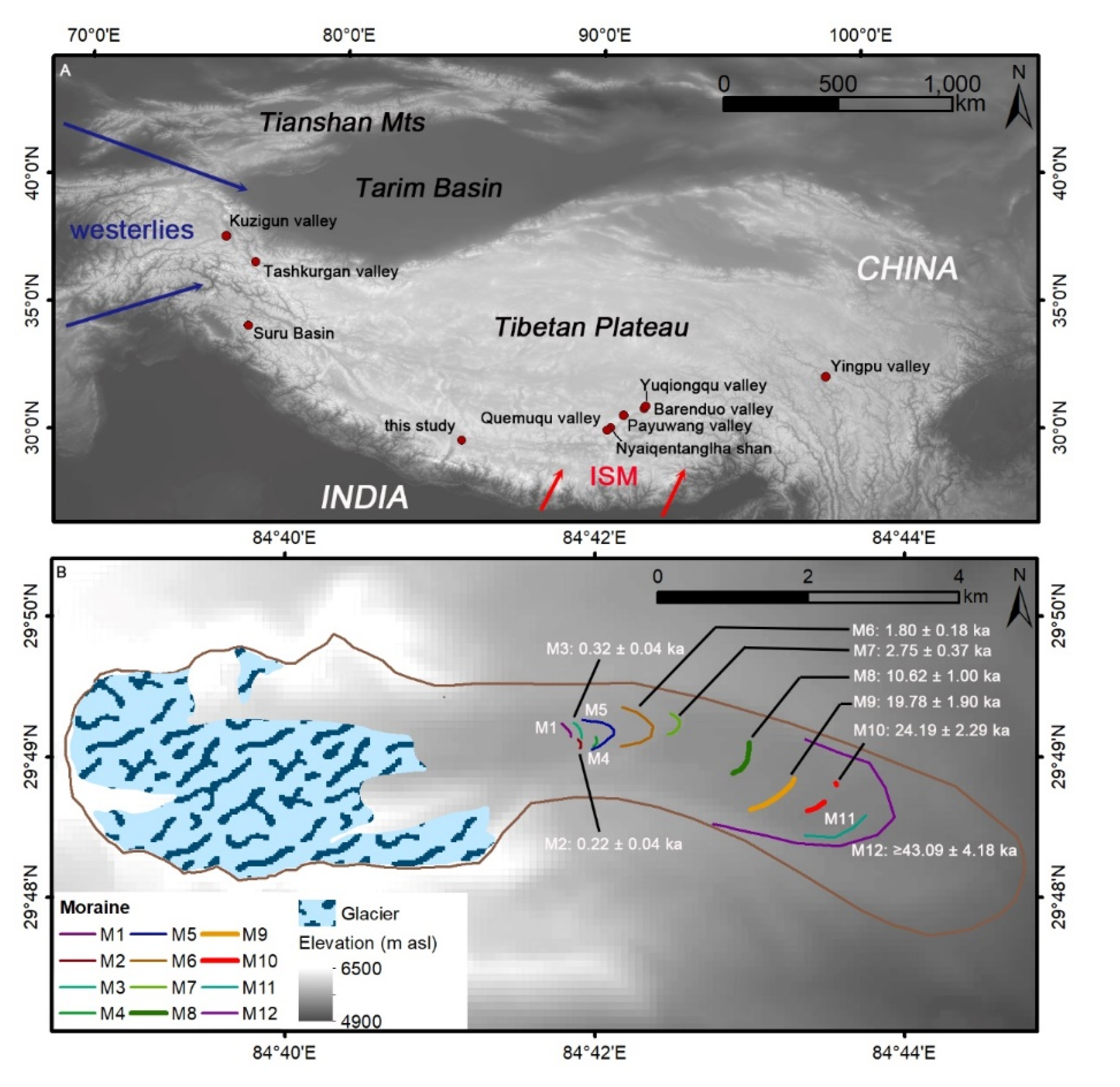
2. Study Site
3. Methods
3.1. Model Input
3.2. Mass Balance Model
3.3. Ice Flow Model
3.4. Modelling Strategy
4. Results
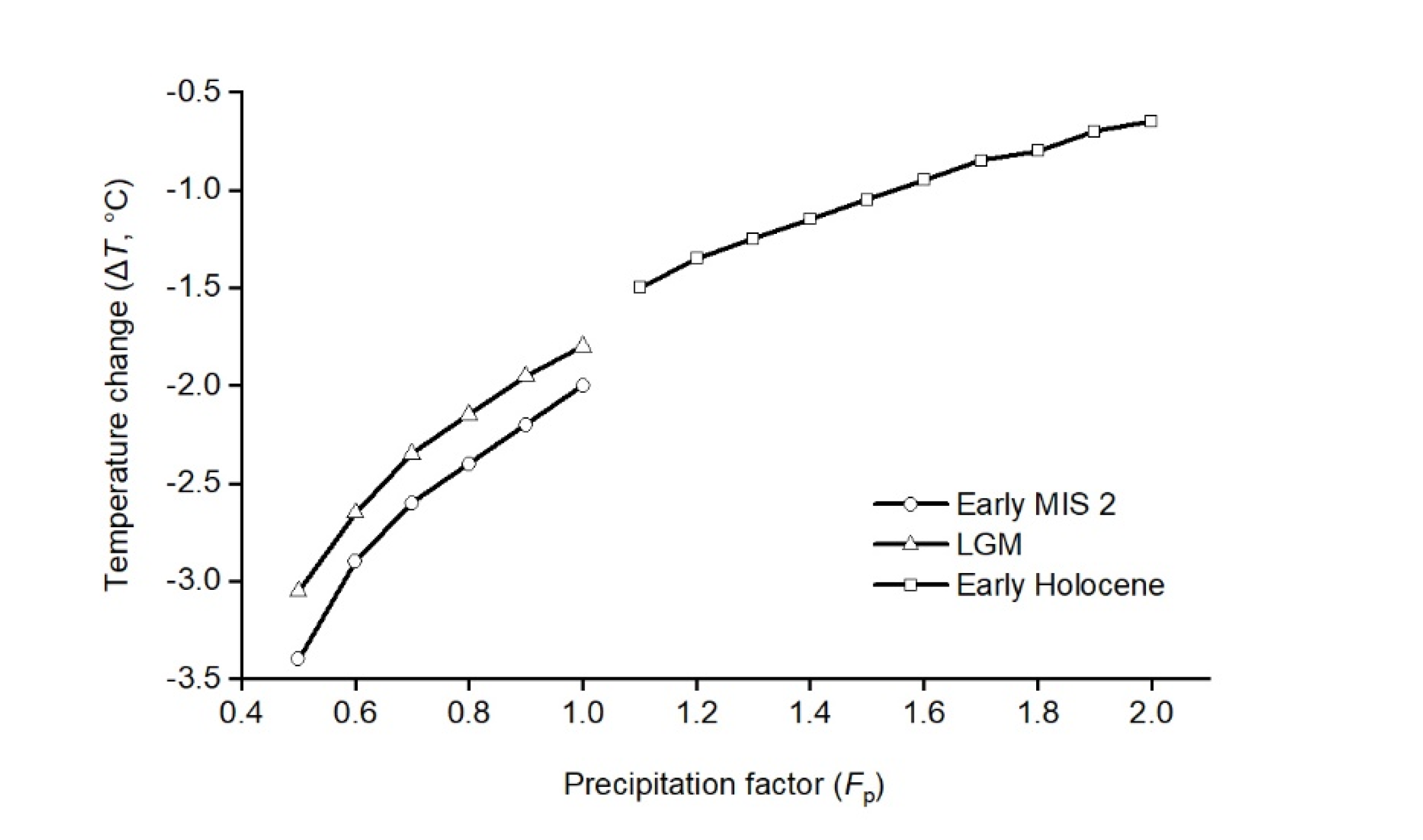
4.1. Early MIS 2
4.2. LGM
4.3. Early Holocene
4.4. Sensitivity Test
5. Discussion
5.1. Sensitivity Analysis
5.2. Palaeoclimate during the Early MIS 2, LGM, and the Early Holocene
6. Conclusions
Author Contributions
Funding
Data Availability Statement
Acknowledgments
Conflicts of Interest
References
- Yao, T.; Thompson, L.; Yang, W.; Yu, W.; Gao, Y.; Guo, X.; Yang, X.; Duan, K.; Zhao, H.; Xu, B.; et al. Different glacier status with atmospheric circulations in Tibetan Plateau and surroundings. Nat. Clim. Chang. 2012, 2, 663–667. [Google Scholar] [CrossRef]
- Zhang, Q.; Yi, C.; Dong, G.; Fu, P.; Wang, N.; Capolongo, D. Quaternary glaciations in the Lopu Kangri area, central Gangdise Mountains, southern Tibetan Plateau. Quat. Sci. Rev. 2018, 201, 470–482. [Google Scholar] [CrossRef]
- Murari, M.K.; Owen, L.A.; Dortch, J.M.; Caffee, M.W.; Dietsch, C.; Fuchs, M.; Haneberg, W.C.; Sharma, M.C.; Townsend-Small, A. Timing and climatic drivers for glaciation across monsoon-influenced regions of the Himalayan–Tibetan orogen. Quat. Sci. Rev. 2014, 88, 159–182. [Google Scholar] [CrossRef]
- Owen, L.A.; Dortch, J.M. Nature and timing of Quaternary glaciation in the Himalayan–Tibetan orogen. Quat. Sci. Rev. 2014, 88, 14–54. [Google Scholar] [CrossRef]
- Heyman, J. Paleoglaciation of the Tibetan Plateau and surrounding mountains based on exposure ages and ELA depression estimates. Quat. Sci. Rev. 2014, 91, 30–41. [Google Scholar] [CrossRef]
- Chevalier, M.-L.; Hilley, G.; Tapponnier, P.; Van Der Woerd, J.; Liu-Zeng, J.; Finkel, R.C.; Ryerson, F.J.; Li, H.; Liu, X. Constraints on the late Quaternary glaciations in Tibet from cosmogenic exposure ages of moraine surfaces. Quat. Sci. Rev. 2011, 30, 528–554. [Google Scholar] [CrossRef]
- Dong, G.; Zhou, W.; Yi, C.; Fu, Y.; Zhang, L.; Li, M. The timing and cause of glacial activity during the last glacial in central Tibet based on 10Be surface exposure dating east of Mount Jaggang, the Xainza range. Quat. Sci. Rev. 2018, 186, 284–297. [Google Scholar] [CrossRef]
- Dong, G.; Zhou, W.; Yi, C.; Zhang, L.; Li, M.; Fu, Y.; Zhang, Q. Cosmogenic 10Be surface exposure dating of “Little Ice Age” glacial events in the Mount Jaggang area, central Tibet. Holocene 2017, 27, 1516–1525. [Google Scholar] [CrossRef]
- Rades, E.F.; Hetzel, R.; Strobl, M.; Xu, Q.; Ding, L. Defining rates of landscape evolution in a south Tibetan graben with in situ-produced cosmogenic 10Be. Earth Surf. Processes Landf. 2015, 40, 1862–1876. [Google Scholar] [CrossRef]
- Liu, X.; Xu, Q.; Ding, L. Differential surface uplift: Cenozoic paleoelevation history of the Tibetan Plateau. Sci. China Earth Sci. 2016, 59, 2105–2120. [Google Scholar] [CrossRef]
- Zhang, Q.; Yi, C.; Fu, P.; Wu, Y.; Liu, J.; Wang, N. Glacier change in the Gangdise Mountains, southern Tibet, since the Little Ice Age. Geomorphology 2018, 306, 51–63. [Google Scholar] [CrossRef]
- Li, Y.; Li, Y.; Chen, Y.; Lu, X. Presumed Little Ice Age glacial extent in the eastern Tian Shan, China. J. Maps 2016, 12, 71–78. [Google Scholar] [CrossRef]
- Loibl, D.; Lehmkuhl, F.; Grießinger, J. Reconstructing glacier retreat since the Little Ice Age in SE Tibet by glacier mapping and equilibrium line altitude calculation. Geomorphology 2014, 214, 22–39. [Google Scholar] [CrossRef]
- Plummer, M.A.; Phillips, F.M. A 2-D numerical model of snow/ice energy balance and ice flow for paleoclimatic interpretation of glacial geomorphic features. Quat. Sci. Rev. 2003, 22, 1389–1406. [Google Scholar] [CrossRef]
- Kessler, M.A.; Anderson, R.S.; Stock, G.M. Modeling topographic and climatic control of east-west asymmetry in Sierra Nevada glacier length during the Last Glacial Maximum. J. Geophys. Res. 2006, 111, 2002–2017. [Google Scholar] [CrossRef]
- Doughty, A.M.; Anderson, B.M.; Mackintosh, A.N.; Kaplan, M.R.; Vandergoes, M.J.; Barrell, D.J.A.; Denton, G.H.; Schaefer, J.M.; Chinn, T.J.H.; Putnam, A.E. Evaluation of Lateglacial temperatures in the Southern Alps of New Zealand based on glacier modelling at Irishman Stream, Ben Ohau Range. Quat. Sci. Rev. 2013, 74, 160–169. [Google Scholar] [CrossRef]
- Rowan, A.V.; Brocklehurst, S.H.; Schultz, D.M.; Plummer, M.A.; Anderson, L.S.; Glasser, N.F. Late Quaternary glacier sensitivity to temperature and precipitation distribution in the Southern Alps of New Zealand. J. Geophys. Res. Earth Surf. 2014, 119, 1064–1081. [Google Scholar] [CrossRef]
- Xu, X.; Hu, G.; Qiao, B. Last Glacial Maximum climate based on cosmogenic 10Be exposure ages and glacier modeling for the head of Tashkurgan Valley, northwest Tibetan Plateau. Quat. Sci. Rev. 2013, 80, 91–101. [Google Scholar] [CrossRef]
- Xu, X. Climates during Late Quaternary glacier advances: Glacier-climate modeling in the Yingpu Valley, eastern Tibetan Plateau. Quat. Sci. Rev. 2014, 101, 18–27. [Google Scholar] [CrossRef]
- Xu, X.; Dong, G.; Pan, B. Modelling glacier advances and related climate conditions during the last glaciation cycle in the Kuzigun Valley, Tashkurgan catchment, on the north-west Tibetan Plateau. J. Quat. Sci. 2014, 29, 279–288. [Google Scholar] [CrossRef]
- Xu, X.; Glasser, N.F. Glacier sensitivity to equilibrium line altitude and reconstruction for the Last Glacial cycle: Glacier modeling in the Payuwang Valley, western Nyaiqentanggulha Shan, Tibetan Plateau. Palaeogeogr. Palaeoclimatol. Palaeoecol. 2015, 440, 614–620. [Google Scholar] [CrossRef]
- Xu, X.; Dong, G.; Pan, B.; Hu, G.; Bi, W.; Liu, J.; Yi, C. Late Glacial glacier-climate modeling in two valleys on the eastern slope of Samdainkangsang Peak, Nyaiqentanggulha Mountains. Sci. China Earth Sci. 2016, 60, 135–142. [Google Scholar] [CrossRef]
- Xu, X.; Pan, B.; Dong, G.; Yi, C.; Glasser, N.F. Last Glacial climate reconstruction by exploring glacier sensitivity to climate on the southeastern slope of the western Nyaiqentanglha Shan, Tibetan Plateau. J. Glaciol. 2017, 63, 361–371. [Google Scholar] [CrossRef]
- Xu, X.; Yao, T.; Xu, B.; Zhang, L.; Sun, Y.; Pan, B. Last Glacial Maximum glacier modelling in the Quemuqu Valley, southern Tibetan Plateau, and its climatic implications. Boreas 2020, 49, 286–295. [Google Scholar] [CrossRef]
- Kumar, V.; Mehta, M.; Shukla, A.; Kumar, A.; Garg, S. Late Quaternary glacial advances and equilibrium-line altitude changes in a semi-arid region, Suru Basin, western Himalaya. Quat. Sci. Rev. 2021, 267, 107100. [Google Scholar] [CrossRef]
- Zhang, Q.; Fu, P.; Yi, C.L.; Wang, N.L.; Wang, Y.T.; Capolongo, D.; Zech, R. Palaeoglacial and palaeoenvironmental conditions of the Gangdise Mountains, southern Tibetan Plateau, as revealed by an ice-free cirque morphology analysis. Geomorphology 2020, 370, 107391. [Google Scholar] [CrossRef]
- Farinotti, D.; Huss, M.; Fürst, J.J.; Landmann, J.; Machguth, H.; Maussion, F.; Pandit, A. A consensus estimate for the ice thickness distribution of all glaciers on Earth. Nat. Geosci. 2019, 12, 168–173. [Google Scholar] [CrossRef]
- Wang, X.; Tolksdorf, V.; Otto, M.; Scherer, D. WRF-based dynamical downscaling of ERA5 reanalysis data for High Mountain Asia: Towards a new version of the High Asia Refined analysis. Int. J. Climatol. 2020, 41, 743–762. [Google Scholar] [CrossRef]
- Braithwaite, R.J. Positive degree-day factors for ablation on the Greenland ice sheet studied by energy-balance modelling. J. Glaciol. 1995, 41, 153–160. [Google Scholar] [CrossRef]
- Hock, R. Temperature index melt modelling in mountain areas. J. Hydrol. 2003, 282, 104–115. [Google Scholar] [CrossRef]
- Anderson, B.; Lawson, W.; Owens, I.; Goodsell, B. Past and future mass balance of “Ka Roimata o Hine Hukatere” Franz Josef Glacier, New Zealand. J. Glaciol. 2006, 52, 597–607. [Google Scholar] [CrossRef]
- Plummer, M.; Socorro, J. Paleoclimatic conditions during the last deglaciation inferred from combined analysis of pluvial and glacial records. PhD thesis, New Mexico Institute of Mining and Technology, Socorro, New Mexico, 2002; p. 346. [Google Scholar]
- Laabs, B.J.C.; Plummer, M.A.; Mickelson, D.M. Climate during the Last Glacial Maximum in the Wasatch and southern Uinta Mountains inferred from glacier modeling. Geomorphology 2006, 75, 300–317. [Google Scholar] [CrossRef]
- Berger, A.; Loutre, M.F. Insolation values for the climate of the last 10 million years. Quat. Sci. Rev. 1991, 10, 297–317. [Google Scholar] [CrossRef]
- Lisiecki, L.E.; Raymo, M.E. A Pliocene-Pleistocene stack of 57 globally distributed benthic δ18O records. Paleoceanography 2005, 20, 1003–1020. [Google Scholar] [CrossRef]
- Zhao, Y.; An, C.-B.; Mao, L.; Zhao, J.; Tang, L.; Zhou, A.; Li, H.; Dong, W.; Duan, F.; Chen, F. Vegetation and climate history in arid western China during MIS2: New insights from pollen and grain-size data of the Balikun Lake, eastern Tien Shan. Quat. Sci. Rev. 2015, 126, 112–125. [Google Scholar] [CrossRef]
- Shukla, T.; Mehta, M.; Jaiswal, M.K.; Srivastava, P.; Dobhal, D.P.; Nainwal, H.C.; Singh, A.K. Late Quaternary glaciation history of monsoon-dominated Dingad basin, central Himalaya, India. Quat. Sci. Rev. 2018, 181, 43–64. [Google Scholar] [CrossRef]
- Shen, C.; Tang, L. Vegetation and climate during the last 250,000 years in Zoige region. Acta Micropalaeontol. Sin. 1996, 13, 373–385, (In Chinese with English abstract). [Google Scholar]
- Thompson, L.G.; Yao, T.; Davis, M.E.; Henderson, K.A.; Mosley-Thompson, E.; Lin, P.N.; Beer, J.; Synal, H.A.; Cole-Dai, J.; Bolzan, J.F. Tropical climate instability: The Last Glacial cycle from a Qinghai-Tibetan ice core. Science 1997, 276, 1821–1825. [Google Scholar] [CrossRef]
- Shi, Y. Discussion on temperature lowering values and equibrium line altitude in the Qinghai-Xizang Plateau during the Last Glacial Maximum and their simulated results. Quat. Sci. 2002, 22, 312–322, (In Chinese with English abstract). [Google Scholar]
- An, Z.; Colman, S.M.; Zhou, W.; Li, X.; Brown, E.T.; Jull, A.J.; Cai, Y.; Huang, Y.; Lu, X.; Chang, H.; et al. Interplay between the Westerlies and Asian monsoon recorded in Lake Qinghai sediments since 32 ka. Sci. Rep. 2012, 2, 619. [Google Scholar] [CrossRef]
- Yu, G.; Chen, X.; Liu, J.; Wang, S. Preliminary study on LGM climate simulation and the diagnosis for East Asia. Chin. Sci. Bull. 2001, 46, 364–368. [Google Scholar] [CrossRef]
- Liu, J.; Yu, G.; Chen, X. Palaeoclimate simulation of 21 ka for the Tibetan Plateau and Eastern Asia. Clim. Dyn. 2002, 19, 575–583. [Google Scholar] [CrossRef]
- Zheng, Y.Q.; Yu, G.; Wang, S.M.; Xue, B.; Zhuo, D.Q.; Zeng, X.M.; Liu, H.Q. Simulation of paleoclimate over East Asia at 6 ka BP and 21 ka BP by a regional climate model. Clim. Dyn. 2004, 23, 513–529. [Google Scholar] [CrossRef]
- Ju, L.; Wang, H.; Jiang, D. Simulation of the Last Glacial Maximum climate over East Asia with a regional climate model nested in a general circulation model. Palaeogeogr. Palaeoclimatol. Palaeoecol. 2007, 248, 376–390. [Google Scholar] [CrossRef]
- Shi, Y.; Zheng, B.; Yao, T. Glaciers and environments during the Last Glacial Maximum (LGM) on the Tibetan Plateau. J. Glaciol. Geocryol. 1997, 19, 97–113, (In Chinese with English abstract). [Google Scholar]
- Jiang, D.; Liu, Y.; Lang, X. A multi-model analysis of glacier equilibrium line altitudes in western China during the Last Glacial Maximum. Sci. China Earth Sci. 2019, 62, 1241–1255. [Google Scholar] [CrossRef]
- Mathewes, R.W. Evidence for Younger Dryas-age cooling on the North Pacific coast of America. Quat. Sci. Rev. 1993, 12, 321–331. [Google Scholar] [CrossRef]
- Marsicek, J.; Shuman, B.N.; Bartlein, P.J.; Shafer, S.L.; Brewer, S. Reconciling divergent trends and millennial variations in Holocene temperatures. Nature 2018, 554, 92–96. [Google Scholar] [CrossRef]
- Shen, Y.; Liu, G.; Shi, Y. Climate and environment in the Tibetan Plateau during the Younger Dryas cooling event. J. Glaciol. Geocryol. 1996, 18, 219–226, (In Chinese with English abstract). [Google Scholar]
- Ma, Q.; Zhu, L.; Lü, X.; Guo, Y.; Ju, J.; Wang, J.; Wang, Y.; Tang, L. Pollen-inferred Holocene vegetation and climate histories in Taro Co, southwestern Tibetan Plateau. Chin. Sci. Bull. 2014, 59, 4101–4114. [Google Scholar] [CrossRef]
- Chen, F.; Zhang, J.; Liu, J.; Cao, X.; Hou, J.; Zhu, L.; Xu, X.; Liu, X.; Wang, M.; Wu, D.; et al. Climate change, vegetation history, and landscape responses on the Tibetan Plateau during the Holocene: A comprehensive review. Quat. Sci. Rev. 2020, 243, 106444. [Google Scholar] [CrossRef]
- Zhen, Q. Exploring the early Anthropocene: Implications from the long-term human-climate interactions in early China. Mediterr. Archaeol. Archaeom. 2021, 21, 133–148. [Google Scholar] [CrossRef]
- Chen, F.; Xu, Q.; Chen, J.; Birks, H.J.B.; Liu, J.; Zhang, S.; Jin, L.; Kandasamy, S.; Telford, R.; Cao, X.; et al. East Asian summer monsoon precipitation variability since the last deglaciation. Sci. Rep. 2015, 5, 1186. [Google Scholar] [CrossRef] [PubMed]


| Study Site | Modern MAAT (°C) | Modern MAP (mm) | ΔT Change (°C) As a Result of a DDF Change of ±0.5 mm °C−1 Day−1 | Fp Change As a Result of a DDF Change of ±0.5 mm °C−1 Day−1 | ΔT Change (°C) As a Result of a Ts Change of ±1 °C | Fp Change As a Result of a Ts Change of ±1 °C | ELA during the LGM (m asl) | ΔELA (m) (Relative to the Modern ELA) | Temperature Decrease (°C) | Precipitation Relative to Modern Value (%) | References |
|---|---|---|---|---|---|---|---|---|---|---|---|
| Tashkurgan valley | 3 | 68.9 | ±0.6 | ±0.1 | ±0.5 | ±0.1 | 4550–4600 | ~600 | 5–8 | 30–70 | Xu et al. [18] |
| Yingpu valley, Queer Mountains | 6.9 | 623.4 | 4630 | 500 | 4–5.9 | 40–80 | Xu [19] | ||||
| Kuzigun valley, Lyavirdyr Tag | 3.9 | 78.6 | ±0.9 | ±0.25 | ±0.8 | ±0.25 | 5–8 | 30–70 | Xu et al. [20] | ||
| Payuwang valley, Nyaiqentanglha Shan | 0 | 282 | 5410 | 340 | 3.3–4.4 | 30–70 | Xu and Glasser [21] | ||||
| Barenduo valley, Samdainkangsang Peak | 2.06 | 478 | Xu et al. [22] | ||||||||
| Yuqiongqu valley, Samdainkangsang Peak | 2.06 | 478 | Xu et al. [22] | ||||||||
| Nyaiqentanglha Shan | 2.06 | 478 | ±0.65 | ±0.25 | ±0.7 | ±0.25 | ~3.6 | ~50 | Xu et al. [23] | ||
| Quemuqu Valley, Qiongmu Gangri Peak | 2.06 | 479.3 | ±0.55 | ±0.4 | ±0.6 | ±0.2 | 5320–5380 | 350–410 | 3.1–4.3 | 30–70 | Xu et al. [24] |
| Gaerqiong Valley, central Gangdise Mountains | −8 | 544 | ±0.05 | ±0.01 | ±0.1 | ±0.02 | ~5816 | ~124 | 2.15–3.05 | 50–80 | This study |
Publisher’s Note: MDPI stays neutral with regard to jurisdictional claims in published maps and institutional affiliations. |
© 2022 by the authors. Licensee MDPI, Basel, Switzerland. This article is an open access article distributed under the terms and conditions of the Creative Commons Attribution (CC BY) license (https://creativecommons.org/licenses/by/4.0/).
Share and Cite
Jiang, Z.; Zhang, Q.; Xu, H.; Wang, N.; Zhang, L.; Capolongo, D. Palaeoclimate Reconstruction of the Central Gangdise Mountains, Southern Tibetan Plateau, Based on Glacier Modelling. Land 2022, 11, 1314. https://doi.org/10.3390/land11081314
Jiang Z, Zhang Q, Xu H, Wang N, Zhang L, Capolongo D. Palaeoclimate Reconstruction of the Central Gangdise Mountains, Southern Tibetan Plateau, Based on Glacier Modelling. Land. 2022; 11(8):1314. https://doi.org/10.3390/land11081314
Chicago/Turabian StyleJiang, Zihan, Qian Zhang, Hanyue Xu, Ninglian Wang, Li Zhang, and Domenico Capolongo. 2022. "Palaeoclimate Reconstruction of the Central Gangdise Mountains, Southern Tibetan Plateau, Based on Glacier Modelling" Land 11, no. 8: 1314. https://doi.org/10.3390/land11081314
APA StyleJiang, Z., Zhang, Q., Xu, H., Wang, N., Zhang, L., & Capolongo, D. (2022). Palaeoclimate Reconstruction of the Central Gangdise Mountains, Southern Tibetan Plateau, Based on Glacier Modelling. Land, 11(8), 1314. https://doi.org/10.3390/land11081314