How Good Are Global Layers for Mapping Rural Settlements? Evidence from China

Abstract

Global urbanization has brought about a significant transition to rural areas. With the development of remote sensing technologies, land use/land cover (LULC) datasets allow users to analyze the changes in global rural settlements. However, few studies have examined the performances of the LULC datasets in mapping rural settlements. Taking China as the study area, this research selected eight of the latest LULC datasets (ESRI Land Cover, WSF, ESA WorldCover, GHS-BUILT-S2, GISD30, GISA2.0, GLC30, and GAIA) to compare their accuracy for rural settlement detection. Spatial stratified sampling was used for collecting and sampling rural settlements. We conducted omission tests, area comparison, and pixel-based accuracy tests for comparison. The results show that: (1) the performances of the 10 m resolution datasets are better than those of the 30 m resolution datasets in almost all scenarios. (2) the mapping of villages in Western China is a challenge for all datasets. (3) GHS-BUILT-S2 performs the best in almost every scenario, and can allow users to adjust the threshold value for determining a proper range of rural settlement size; ESRI outperforms any other dataset in detecting the existence of rural settlements, but it dramatically overestimates the area of rural settlements. (4) GISD30 is the best among the 30 m resolution datasets, notably in the Pearl River Delta. Finally, we provide useful suggestions on ideal map selection in various regions and scenarios.

1. Introduction

Global urbanization is one of the most overwhelming trends of the 21st century; however, 45 percent of the world’s people still live in rural areas and have been affected by globalization, but have received less attention [1,2]. Facing a significant transition, the United Nations has put forward goals for sustainable rural development, including an increasing investment in rural infrastructure and supporting the facilitation of positive economic, social, and environmental links between urban, peri-urban, and rural areas [3].

A better understanding of the changes in rural settlements can help ensure sustainable rural development. In the literature, extensive studies have analyzed rural settlements. Most of them were conducted on a small scale, such as a single town [4,5], county [6,7,8], or city [9], which require detailed rural settlement data. Some of these studies visually interpreted very high resolution (VHR, <10 m) remote sensing images to extract the rural settlement patches [5,7,8], and some obtained detailed survey data from local authorities [4,6]. The other studies that performed an analysis on a large scale usually aggregated the statistical data at a municipal or provincial level [10]. However, visual interpretations and field surveys are costly and restrict the study scale, and the statistical data from governments lack details and limit refined analyses. Hence, datasets with fine details on a large scale are essential for the study of rural settlements.

With the development of Earth observation satellite technology, land cover information interpreted from remote sensing images has an increasing capacity to reveal the detailed characteristics of human settlements. During the first decade of the new century, a batch of global land use/land cover (LULC) data, such as the Global Rural-Urban Mapping Project (GRUMP) [11] and MODIS Urban Land Cover 500 m (MOD500) [12,13], were employed to monitor urban morphology. The data were usually derived from Moderate Resolution Imaging Spectroradiometer (MODIS) at a 1 km or 500 m resolution [14,15,16], which allowed users to recognize large-scale urban areas, but did not allow for the identification of small rural settlements [17,18]. Since 2013, the resolution of several global LULC datasets has reached resolutions of 30 m or even 10 m, which enables users to map human settlements with topological details on a large scale. Thus far, a series of high- or moderate-resolution (10–100 m) global maps provide different categories of land information, such as human settlements [19,20], impervious surfaces [21,22,23,24,25,26], artificial surfaces [27], and built-up areas [28,29]. Although the classification standards differ, most of these layers cover rural settlements. However, how accurately do these datasets map the rural settlements? Does the mapping accuracy vary by region? In what circumstance, and to what extent can we use them to delineate rural settlements? In the literature, few studies have been dedicated to answering these questions. Against this background, this study aimed to develop a framework for evaluating the performance of the latest high-resolution LULC datasets in mapping rural settlements using China as the study area.

The sections of this study are organized as follows. Section 2 presents existing research on the widely used LULC datasets and the identification of rural settlements. Section 3 introduces the advantages of choosing China as the study area and provides details on the eight selected LULC datasets. The evaluation framework is introduced in the Methodology section. The main results are presented and discussed in Section 5, followed by conclusions in Section 6.

2. Literature Review

The observation of human settlements, which plays a crucial role in human-related studies, has become an important research scope in remote sensing studies. With the development of remote sensing technologies and computational capacities, global human settlement datasets have been produced, ranging from coarse resolution (>500 m) to high resolution (10–30 m) in recent years.

Table 1. Overview of the 16 rural-related global LULC datasets.

Abbr.	Map	Producer	Resolution	Earliest/Latest Release Time	Time Cover	Map Type	Map Representations Related to Rural Settlement	Primary Data Sources
ESRI Land Cover	Sentinel-2 10 m Land Use/Land Cover	ESRI	10 m	2021/2022	2017–2021	Thematic (10 classes)	Built-up area	Sentinel-2
WSF	World Settlement Footprint	European Space Agency (ESA) and the German Aerospace Center (DLR)	10 m	2020/2021	2015; 2019	Binary (settlement/not settlement)	Human settlement	Sentinel-1 and Landsat 8
WorldCover	ESA WorldCover	European Space Agency (ESA)	10 m	2021	2020	Thematic (11 classes)	Impervious surface	Sentinel-1 and Sentinel-2
GHS-BUILT-S2 (from the GHSL series)	Global Human Settlement Layer Built-up Grid Derived from Sentinel-2 Global Image	European Commission-Joint Research Centre	10 m	2020	2018	Continuous (built-up probability values)	Built-up area	Sentinel-2
FROM-GLC10	Finer Resolution Observation and Monitoring of Global Land Cover	Tsinghua University	10 m; 30 m	2019	2017	Thematic (10 classes)	Impervious surface	Sentinel-2
GUF	Global Urban Footprint	German Remote Sensing Data Center (DFD)	12 m	2017	2011	Binary (settlement/not settlement)	Human settlement	TerraSAR-X and TanDEM-X
GISD30	Global 30 m Impervious Surface Dynamic Dataset	Aerospace Information Research Institute, Chinese Academy of Sciences	30 m	2022	1985–2020	Continuous (built year values)	Impervious surface	Landsat 4, 5, 7 and 8
GISA2.0	Global Impervious Surface Area 2.0	Wuhan University	30 m	2022	1972–2019	Continuous (built year values)	Impervious surface	GISA1.0, GAIA, GAUD, GHSL
GLC30	GlobeLand30	National Geomatics Center of China	30 m	2014/2021	2000; 2010; 2020	Thematic (10 classes)	Artificial surface	Landsat Series (2000; 2010; 2020) and GF-1 (only 2020 version)
GAUD	Global Annual Urban Dynamics	Global Annual Urban Dynamics	30 m	2020	1985–2015	Continuous (built year values)	Urban area	Landsat Series
GAIA	Annual Maps of Global Artificial Impervious Area	Tsinghua University	30 m	2019	1978–2018	Continuous (built year values)	Impervious surface	Landsat Series
GMIS	Global Man-made Impervious Surface	NASA Goddard Space Flight Center and the Department of Geographical Sciences at the University of Maryland	30 m	2017	2010	Continuous (impervious surface percentage)	Impervious surface	Landsat Series
HBASE	Global Human Built-up And Settlement Extent		30 m	2017	2010	Binary (HBASE/ROAD/not HBASE); Continuous (HBASE percentage)	Built-up area	Landsat Series
MGUP	MODIS Global Urban Extent Product	Wuhan University	250 m	2021	2001–2018	Binary (urban area/not urban area)	Urban area	MODIS
MCD12Q1 v6	The MODIS Land Cover Type Product	Land Processes Distributed Active Archive Center (LP DAAC)	500 m	2019/2021	2000–2020	Thematic (17 classes)	Urban and Built-up Lands	MODIS
MOD500	MODIS 500m Map of Global Urban Extent	University of Wisconsin and Boston	500 m	2009	2001/2002	Binary (urban area/not urban area)	Urban area	MODIS

lists the recent human settlement observation datasets, sorted by resolution and release time. No global datasets covering human settlements were extracted by VHR remote sensing images, such as World View, IKONOS, and Quick Birds, because of their high costs in mass data acquisition, storage, and calculation complexity [19,30,31]. Moderate and coarse datasets, such as MCD12Q1 [16] and MOD500 [12], were derived from a relatively low-resolution data source (MODIS, 250–1000 m); they have difficulties in detecting small human settlements because the scale of the scattered built-up area can be 10–20 m, despite regional variation [32]. Although the mixed pixels still appear in high-resolution images, 10–30 m resolution worldwide LULC datasets have nowadays proven themselves to be better choices in mapping human settlements [19,33]. Among them, GISA2.0 was generated from multi-source LULC maps; the others can be divided into passive optical (Landsat series, Sentinel-2) and active radar (Sentinel-1, TerraSAR-X, TanDEM-X) products in terms of primary data sources, both of which face challenges in the mapping of human settlements [19,33]. Spectral confusion and seasonal changes in ground objects can negatively influence the performance of optical maps. Due to the similarity of spectral features, misclassifications often occur between sand (or sandy soil) and concrete surfaces. The same goes for shrubbery and low or old buildings [34,35]. The influence of seasonal factors is mainly reflected in the soil moisture assay and ground surface temperature, which is related to the climate and soil type [34]. The influence is even greater on maps such as GHSL and GLC30, which were generated from single-date optical scenes [19]. For active radar products, object height is a primary influential factor [33]. For example, GUF may misclassify forest regions as rural settlements due to their similar low backscattering signals [36].

In the literature, rural settlements have received far fewer concerns than urban places [17,18]. Several studies developed methods to map rural settlements [37,38,39], but they targeted small-scale regions. Although no rural-specific dataset has been produced on a global scale, human settlements detected by many global LULC datasets at 10 m or 30 m resolutions cover rural settlements. However, there is limited research that has focused on validating these products in their mapping of rural settlements. An exception is Matthias et al. [36], who validated the accuracy of the GUF in a rural area in Burkina Faso. They found that the GUF presents a 50.9% correctness in a low building-dense condition, which performs better than the GHSL Landsat (beta) (14.86% correctness). Another study by Klotz et al. [18] examined two cities and the nearby rural areas in Central Europe. They confirmed the ability of the GUF and GHSL (the earlier version of GHS-BUILT-S2) in identifying small settlement fragments compared with low-resolution LULC data. However, these studies only evaluated two high-resolution datasets and concentrated on a small area while neglecting the types of rural settlements and regional variation. It is necessary to evaluate the performance of the latest LULC datasets in their mapping of different types of rural settlements on a larger scale.

3. Study Area and Data

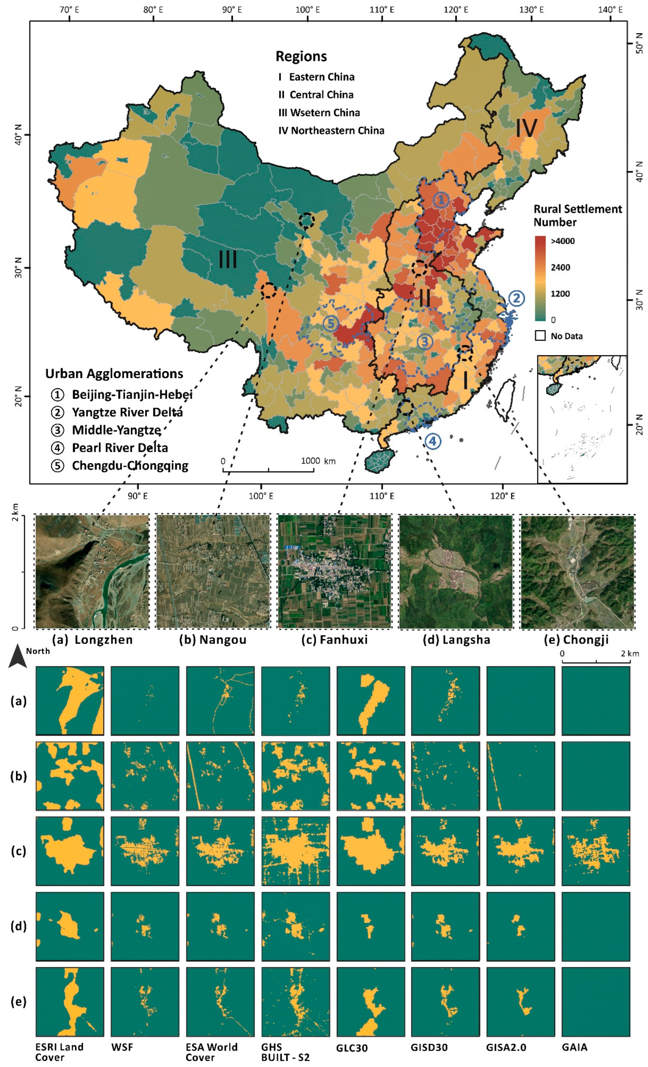
3.1. Study Area

We chose China (see Figure 1) as the study area because of its vast territory and diverse rural settlements [40]. It has different ground and house materials, elevation, and settlement density that may significantly influence the mapping accuracy. Another reason we rely on the evidence from China is that we can obtain reliable rural settlement data for validation. Since 2009, the National Bureau of Statistics of China (NBSC) has annually published the latest zoning codes and urban-rural division codes, which allowed us to obtain the names and locations of rural settlements within the whole territory [41].

3.2. Data

The classification criteria proposed by the NBSC in 2008 introduced four types of rural-related units: city fringe, town fringe, township, and village [42]. City fringe and town fringe cover both urban and rural settlements; hence, rural settlements in city fringes and town fringes are more likely to have features that are similar to urban settlements. Both townships and villages can be regarded as rural settlements; the former are larger and have more continuous built-up areas than the latter. This study introduced four types of units because they all cover types of rural settlements. We collected the names of settlements and their zoning codes from the 2021 data, and we used an online geocoding service to map the settlement locations. Each point represents the respective seat in government, which is usually located in the center of the unit. In 2021, the number of registered rural-related units was 487,524, where 6.06% were city fringes, 11.22% were town fringes, 2.41% were townships, and 80.31% were villages. Figure 1 describes the spatial distribution of rural settlements at the prefectural level. It can be observed that most of the rural settlements were distributed in Eastern and Central China.

Eight of sixteen global LULC maps in Table 1 were selected as target layers for accuracy tests, including the ESRI Land Cover, WSF, ESA WorldCover, GHS-BUILT-S2, GISD, GISA2.0, GLC30, and GAIA. Among the exclusions, the GMIS and HBASE only describe the scenes from 2010, which would be difficult to compare with products that were produced around 2020 [26,43]. The GUF [20] and GROM-GLC10 [44] were the earlier products from the same research groups of WSF and GAIA, respectively. The GAUD [45], MGUP [46], MCD12Q1 v6 [16], and MOD500 [12] focused on the identification of urban areas, which were beyond our research’s scope [45]. Figure 1 introduces Google Earth (GE) images to delineate five typical rural settlements with different functions (village, town fringe, or township) or landforms (plateau, mountainous, plain, or hill). The settlements identified by the eight maps indicated that the ability to detect different types of rural settlements varied by the product used.

One type of dataset refers to those at the resolution of 10 m. The ESRI Land Cover (hereafter called ESRI) was generated from the Sentinel-2 with a deep learning model. The model handles six bands from the Sentinel-2, including green, blue, red, near-infrared, and two short-infrared bands; images from multiple dates were integrated to avoid cloud cover or other adverse effects [28]. The WSF was the first human settlement map to combine optical (Landsat 8) and radar (Sentinel-1) products at a 10 m resolution. Previous research indicated that the WSF had a better performance in detecting small villages and depicting urban boundaries than the GUF (12 m resolution), GHSL (GHS-BUILT 2018 version, 30 m resolution), and GLC30 (30 m resolution) in Igboland (a region located in south-eastern Nigeria), Kampala (the largest city of Uganda), and Bangalore (the capital of the Indian state of Karnataka) [19]. The GHS-BUILT-S2 (hereafter called GHSL) is the latest product of the GHSL series published in 2020 [47]. Its pixel value represents the proportion of built-up area, which is a better solution for handling mixed pixels. The other LULC map is the ESA WorldCover (hereafter called ESA) [22], which was also generated from both optical (Sentinel-2) and radar (Sentinel-1) products. In summary, the ESRI, GHSL, and ESA mainly employed deep learning models to extract the characteristics of ground objects; the WSF focused on texture feature extraction and spectral index construction, and it used the support vector machine model to classify pixels.

The other global LULC maps chosen were produced at a 30 m resolution. The GISD30, GCL30, and GAIA were directly derived from the Landsat Series; GISA2.0 was developed based on existing impervious surface products, including the GISA1.0 [24], GAIA, GAUD, and GHSL. Thanks to the long-time coverage of the Landsat Series, GISD30, GISA2.0, and GAIA can provide a continuous pixel value to represent the built year of each impervious surface pixel, and the earliest year can date back to 1972. For these continuous pixels, we converted them to ensure that the data could represent all of the impervious surfaces of the latest year. For example, in the GISD30, all pixels representing the impervious surface from 1985 to 2020 were considered as the existing impervious surface in 2020 and were converted to the same pixel value.

To construct validation sample units (VSU), we utilized the GE images as a reference layer for a visual interpretation because they have been widely acknowledged as one of the most important data sources for accuracy assessment [14,48,49]. Because the LULC maps were produced in varying years, this study only selected the rural settlements that had not changed significantly in recent years as the samples for accuracy assessment. As ecological and topographical factors significantly affect the identification accuracy of human settlements, we performed a spatial stratified sampling (SSS) by considering ecological [34] and geomorphic [50] effects. We used Shuttle Radar Topography Mission 3 v4.1 (SRTM3 v4.1), a digital elevation model (DEM) with a 90 m resolution released by NASA [51], to measure the similarities between rural settlements.

4. Methodology

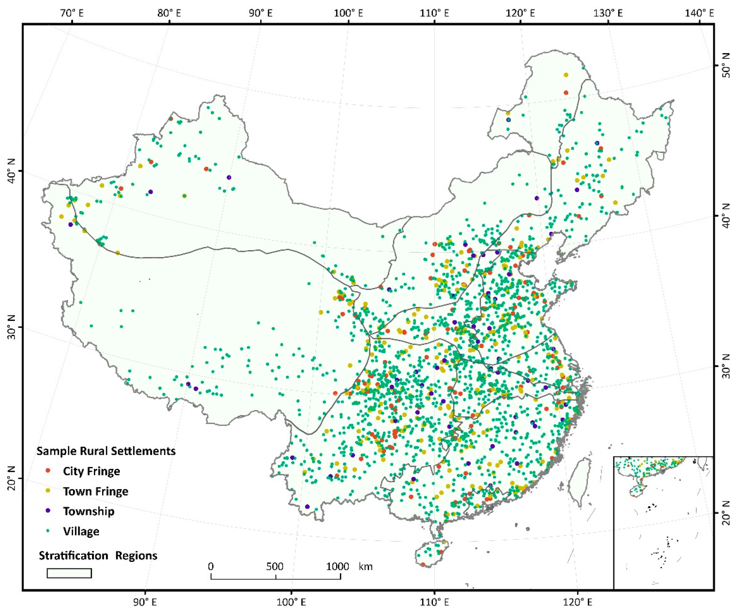
4.1. Method of Sampling

Rural settlements are typical geospatial objects whose spatial autocorrelation is reflected in their similar natural, economic, and cultural characteristics among neighboring units [52]. The significant positive spatial autocorrelation does not satisfy the independence hypothesis of classical sampling theory. Similar samples that contain overlapping information result in the loss of samples used for effective estimation [53,54]. In China, a typical example is on the North China Plain, where the clusters of villages have similar settlement scales, architectural styles, and natural environments [55]. To consider the spatial autocorrelation and heterogeneity of rural settlements in China, we employed spatial stratified sampling techniques to sample the rural settlements.

The SSS was developed from the classical stratified sampling method. The SSS requires a minimum variance within layers and a maximum variance between layers, and it also considers the space continuity of objects within the same layer. The selection of prior knowledge for the stratification is crucial to benefit the effect of SSS. As the optical sensors and radar are sensitive to ecological and topographical environments, we obtained the stratified layer for sampling by integrating an ecological regionalization layer [34] and a geomorphic zoning layer [50].

The total sample size of the entire study area was calculated by simple random sampling. When the population is infinite or unknown, the sample size (ss) can be calculated by giving the confidence level and confidence interval:

$$ss=\frac{Z^{2}p\left(1-p\right)}{c^2},$$

(1)

where $Z$ is the Z value (e.g., 1.96 means a 95% confidence level), $p$ is the percentage of picking a choice (which is often set to 0.5 by default), and $c$ is the confidence interval (e.g., 0.04 = $\pm 4$). When the population is known and finite, the sample size can be modified using:

$$new ss=\frac{ss}{1+\frac{ss-1}{pop}},$$

(2)

where $new ss$ is the modified sample size and $pop$ is the number of the population.

Next, we distributed the total samples to each stratification region according to the weights. As elevation is another influencing factor [39], we created a 1 km buffer around each rural settlement and calculated the elevation range within the buffer, whereby the similarity of samples within a stratification region could be measured. Meanwhile, to reduce redundant information among sample points in each stratification region, we used Neiman allocation [56] to determine the sample size of each region, which is determined by:

$$n_h=n\times \frac{N_h{S}_h}{{\displaystyle \sum }{N}_h{S}_h},$$

(3)

where $n_h$ is the sample size of the $h$th region, $n$ is the total sample size, $N_h$ is the number of rural settlements within the $h$th region, and $S_h$ is the standard deviation of the elevation range in the $h$th region.

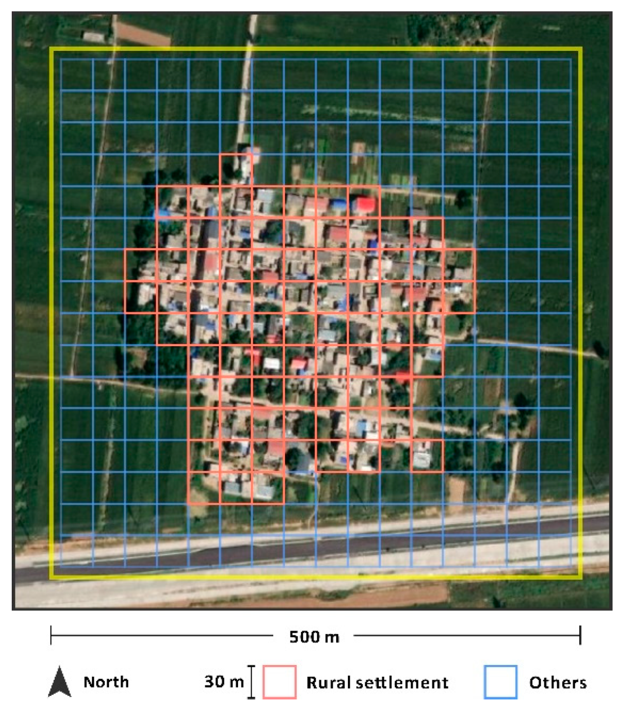
4.2. Establishment of Validation Sample Units

The location of each sampling point provided by the NBSC was examined with the GE images to ensure that it was located in a rural settlement. VSUs were then constructed after the validation procedure. Figure 2 shows an example of a VSU. Two tiers of validation grids were placed over each rural settlement, and were centered on the location of the sampling point. One tier contained 500 m $\times$ 500 m grids, which fit the common coarse-resolution products, such as the MOD500 or MCD12Q1. The size was large enough to roughly cover the rural settlement patches because the average patch size of a rural settlement in China is 16.27 hectares [55]. The grids were used to examine whether LULC maps omitted the entire rural settlement. The grids in another tier were created at a resolution of 30 m and grouped into a 16 $\times$ 16 square for one rural settlement to fill an approximately 500 m $\times$ 500 m grid. When pixel-based analyses were performed in these 30 m $\times$ 30 m grids, 10 m resolution datasets were resampled to 30 m resolution maps to match the grid size. Following previous studies’ methodology on the accuracy assessment of mapping urban settlements [17,18], a grid containing more than 50% of the built-up area in the GE images was considered rural. In addition, the inner country roads (the roads covered by rural settlement pixels in Figure 2) were treated as rural settlements to ensure morphological integrity. Meanwhile, historical images of each site were used to ensure that there had been no significant changes over the past five years, which would make LULC maps from different years comparable.

In addition to rural settlement types (city fringe, town fringe, township, and village), we applied four regions [57] (Northeastern, Eastern, Central, and Western China) and five urban agglomerations (Beijing–Tianjin–Hebei, Yangtze River Delta, Middle Yangtze, Pearl River Delta, and Chengdu–Chongqing) [58] in China (see Figure 1) to further explore the regional variation in the identification accuracy of these products.

4.3. Accuracy Assessment Indicators

Overall accuracy assessments, including omission and area tests, were applied to the eight maps. A rural settlement was identified as omitted when the map had no settlement pixel within the 500 m $\times$ 500 m grid of the corresponding VSU. For the area tests, we calculated the area of pixels in each VSU.

Pixel-based accuracy assessments were performed by following the pixel-based error matrix in

Table 2. Conceptualization of the pixel-based error matrix.

		Map Under Test
		Presence	Absence
Reference map	Presence	True Positive (TP)	False Negative (FN)
	Absence	False Positive (FP)	Ture Negative (TN)

.

Following Foody’s recommendations [59], we employed overall accuracy (OA, Equation (4)), producer’s accuracy (PA, Equation (5)), user’s accuracy (UA, Equation (6)), and F-score (F, Equation (7)) equations:

$$OA=\frac{TP+TN}{TP+TN+FP+FN},$$

(4)

$$PA=\frac{TP}{TP+FN},$$

(5)

$$UA=\frac{TP}{TP+FP},$$

(6)

$$F=\frac{2TP}{2TP+FP+FN},$$

(7)

Among them, OA represents the total proportion of correctly classified pixels. PA and UA are also referred to in data science as “recall” and “precision”, respectively. The former emphasizes whether all rural settlement pixels can be found, and the latter considers the probability that all rural settlement pixels in the region are correctly classified. In general, PA and UA are negatively correlated. The F-score can be regarded as a balanced value of PA and UA, representing the comprehensive accuracy of the map under the test. Note that the famous Cohen’s kappa coefficient was not adopted in our study because it is quite sensitive to multi-categories. In the case of rural settlement identification, we were not concerned about other types of land. The number of rural settlement pixels varied significantly among VSUs, reducing the comparability of kappa coefficients.

5. Results

5.1. Sampling

The whole study area was divided into 12 stratification regions using the SSS method. Following Equation (2), setting 95% as the confidence level and 2% as the confidence interval, the sample size was calculated to be 2376, with a population size of 487,524. The stratification regions and sample rural settlements are shown in Figure 3.

5.2. Accuracy Assessment

5.2.1. Omission Test

Table 3. Sample rural settlements omitted by the eight LULC maps.

	ESA	ESRI	GHSL *	WSF	GAIA	GISA2.0	GISD30	GLC30	8-Map Mean
Total Omissions	126	87	92	190	1148	723	347	862	446.88
Omission rate (%)	5.41	3.74	3.95	8.17	49.33	31.07	14.91	37.04	19.2
(a) By Type (%)										Class Size
City Fringe	0.69	0	0.68	1.38	11.03	7.59	0.69	11.72	4.22	145
Town Fringe	1.89	0.75	1.13	1.89	31.7	14.34	5.28	24.15	10.14	265
Township	0	0	1.72	3.45	56.9	18.97	8.62	17.24	13.36	58
Village	6.46	4.57	4.67	9.74	54.6	35.66	17.59	41.47	21.85	1859
(b) By region (%)
Eastern China	0.32	1.74	0.15	1.74	25.24	11.51	3.79	16.72	7.65	634
Central China	2.7	1.95	0.45	4.05	40.93	19.04	11.54	37.03	14.71	667
Western China	11.35	6.64	9.42	16.17	74.73	54.82	26.02	53.32	31.56	934
Northeastern China	0	1.09	0	1.09	18.48	11.96	3.26	11.96	5.98	92
(c) By Urban Agglomeration (%)
Beijing-Tianjin-Hebei	0.65	5.84	0.65	1.3	26.62	18.83	5.84	8.44	8.52	154
Chengdu-Chongqing	7.37	1.05	0.52	10.53	66.32	47.89	23.16	70	28.36	190
Middle-Yangtze	2.67	0.89	0.44	1.33	45.78	17.78	11.56	50.67	16.39	225
Pearl River Delta	0	0	0	0	35.48	6.45	0	6.45	6.05	31
Yangtze River Delta	0	0	0	1.41	11.27	4.93	2.11	28.87	6.07	142

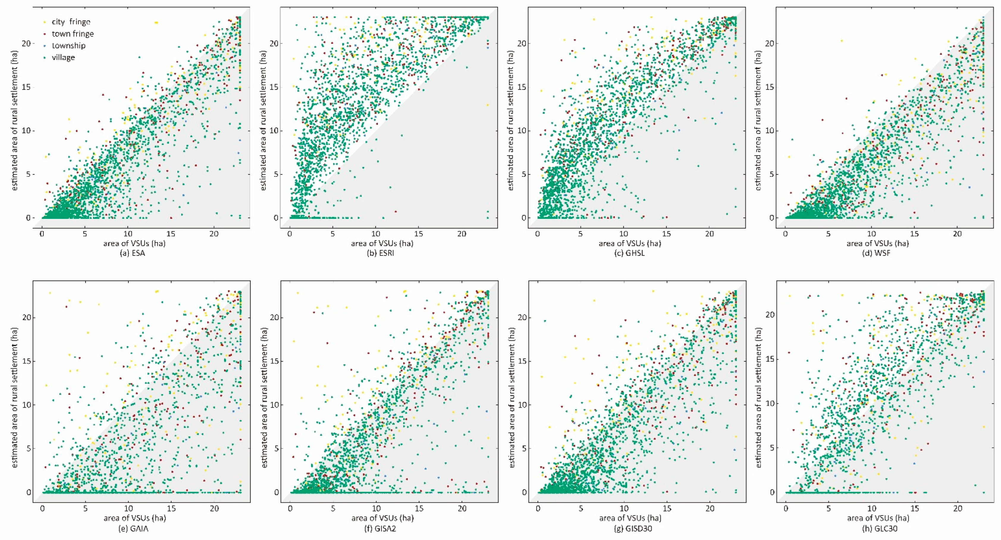
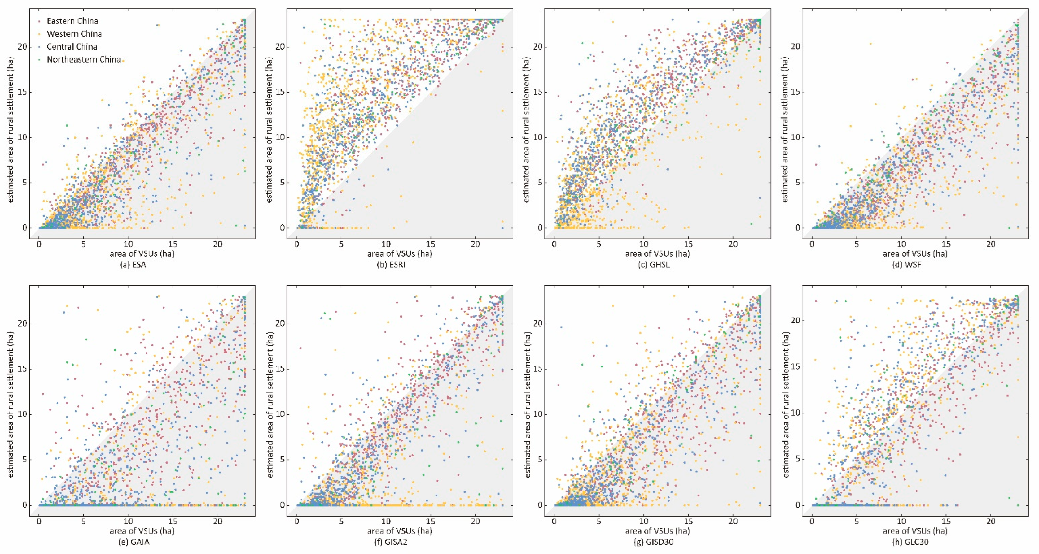
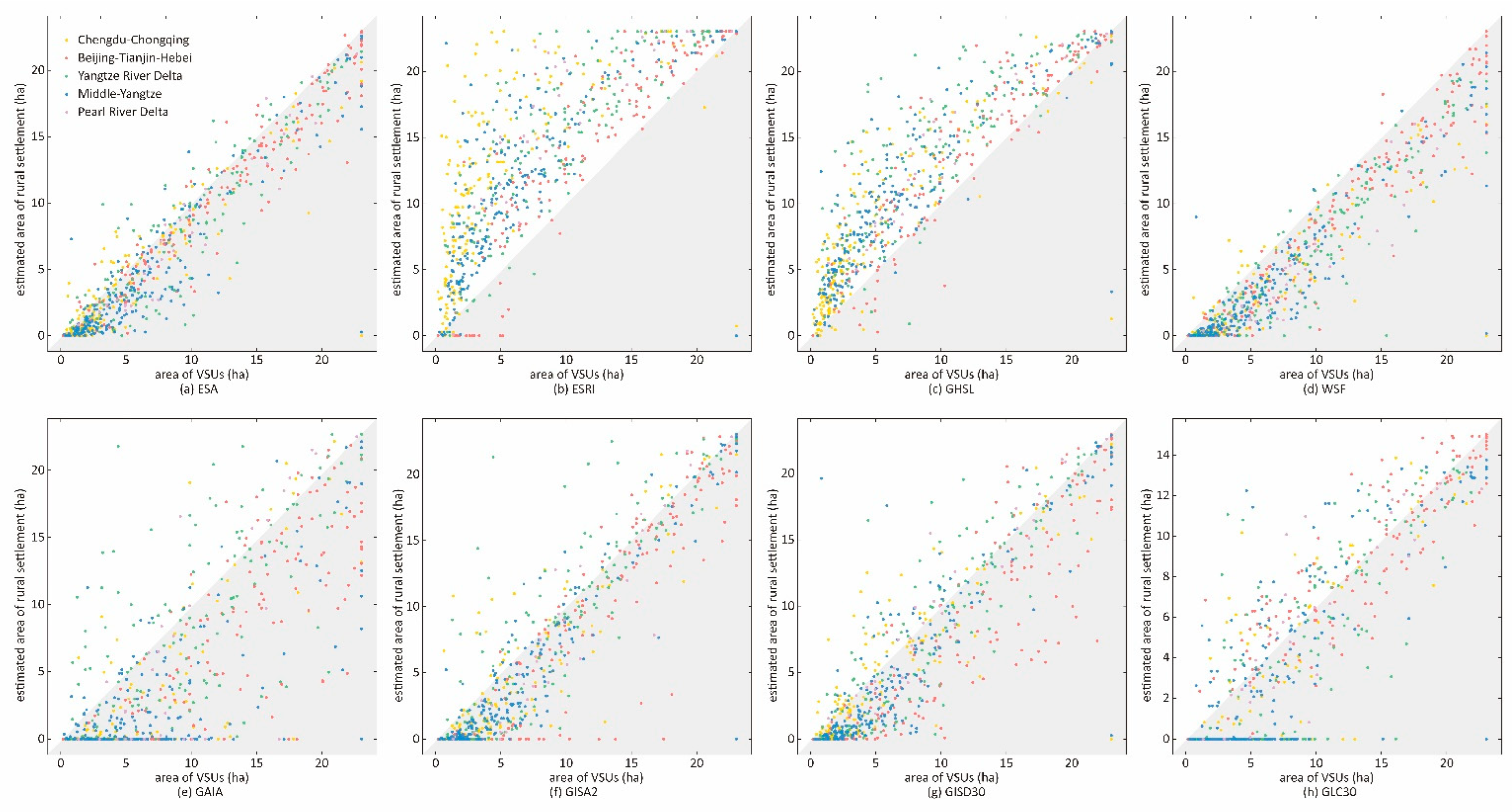
* The rural settlement pixels in the GHSL were extracted at a threshold value of 10%.

shows the results of the omission test. As the GHSL has a continuous value to represent the percentage of built-up area in a pixel, we tested the accuracy of the map in increments of 10%. We finally selected 10% as the threshold value because it had a minimum value in the omission rate. Additionally, we believed that a lower threshold value might help detect scattered small rural settlements.

For the total omissions, all four maps at 10 m resolutions (ESA, ESRI, GHSL, WSF) had an omission rate smaller than 10%, indicating that they could identify the existence of rural settlements in China. Among them, the ESRI reached the lowest omission rate (3.74%), followed by the GHSL (3.95%), ESA (5.41%), and WSF (8.17%). However, the omission rates of maps at 30 m resolutions were significantly higher than those of 10 m resolution products.

Villages had the highest omission rates for all maps, probably due to the fragmented built-up area. Maps at 10 m resolution had outstanding performances for city fringes, town fringes, and townships, with the omission rates scoring lower than 5%. The performances of the four maps at 30 m resolution were inferior to the 10 m resolution products, regardless of the settlement type. An exception was the GISD30, which performed well in mapping the rural settlements of city fringes with an omission rate equal to 0.69%.

The omission rates of rural settlements in Northeastern China and Eastern China were relatively low, probably because a large share of the rural settlements in the two regions were plain and relatively well-developed. Western China provided the highest omission rate in all maps, probably due to more the bare lands, mountains, and discrete patterns of rural houses. Similar findings were observed in urban agglomeration comparison. The maps performed significantly better in three of the eastern urban agglomerations (the Pearl River Delta, the Yangtze River Delta, and the Beijing–Tianjin–Hebei) than in the central and western urban agglomerations (Middle Yangtze and Chengdu–Chongqing). Among the eastern urban agglomerations, the omission rate of the ESRI achieved 0% in the Yangtze River Delta and Pearl River Delta urban agglomerations, but reached 5.84% in the Beijing–Tianjin–Hebei urban agglomeration, indicating a significant regional variation.

5.2.2. Area Test

Figure 4 shows the area test result by functional type. In each subgraph, the x-axis represents the actual rural settlement area obtained by the visual interpretation in each VSU, and the y-axis represents the rural settlement area identified by each LULC map. Each point represents a VSU. The points that are closer to the (0,0) and (1,1) diagonal show better agreement with the actual area. Meanwhile, the points below (or above) the diagonal indicate that the landcover map underestimated (or overestimated) the rural settlement area. In general, maps at 10 m resolutions either overestimated (The ESRI and GHSL) or underestimated (The ESA and WSF) the rural settlements, whereas dots of maps at 30 m resolutions were dispersed around the diagonals. All maps except the WSF tended to overestimate the area of city fringes, probably due to their connection to urban areas. The ESA had the best performance in city fringes, town fringes, and townships, with a lower random deviation. The green dots that piled up in the lower left corner indicate that small-area villages are likely to be underestimated or omitted. The GHSL and ESRI could capture small villages, but the deviation of the ESRI was extremely large. Therefore, the GHSL is best used to estimate the size of villages. Although it had some slight overestimations, we can adjust the threshold to alleviate the overestimation problem while preserving its ability to capture small villages, due to the continuity of its pixel values.

Figure 5 and Figure 6 illustrate the area test results by region and urban agglomeration, respectively. Western rural settlements, especially tiny rural settlements, are most likely to be omitted and underestimated. This provides additional evidence that rural settlements in Western China are challenges for all LULC maps. For Central China, only GHSL can effectively estimate small and large rural settlements. ESA has advantages in dealing with medium-sized rural settlements. The point patterns of Northeastern China and Eastern China are similar, where ESA, WSF, and GISA2.0 have effective estimations.

In the Beijing–Tianjin–Hebei urban agglomeration, the ESA, GHSL, and WSF effectively detected rural settlements; the ESRI had a high omission rate for small villages under five hectares, and its estimations for large rural settlements were more accurate. In the Yangtze River Delta and Middle Yangtze urban agglomerations, both the ESA and WSF performed well, but the latter had a slight underestimation tendency. The Chengdu–Chongqing urban agglomeration is located in Western China, where the countryside is relatively underdeveloped and the topography is complicated. Small settlements in the urban agglomeration were frequently omitted from LULC maps, except for in the ESRI and GHSL; the ESA and WSF demonstrated superior area estimation skills if the omission rates were ignored. It is worth mentioning that two 30 m resolution maps, namely the GISD30 and GISA2.0, showed pleasing estimation effects in the Pearl River Delta urban agglomeration.

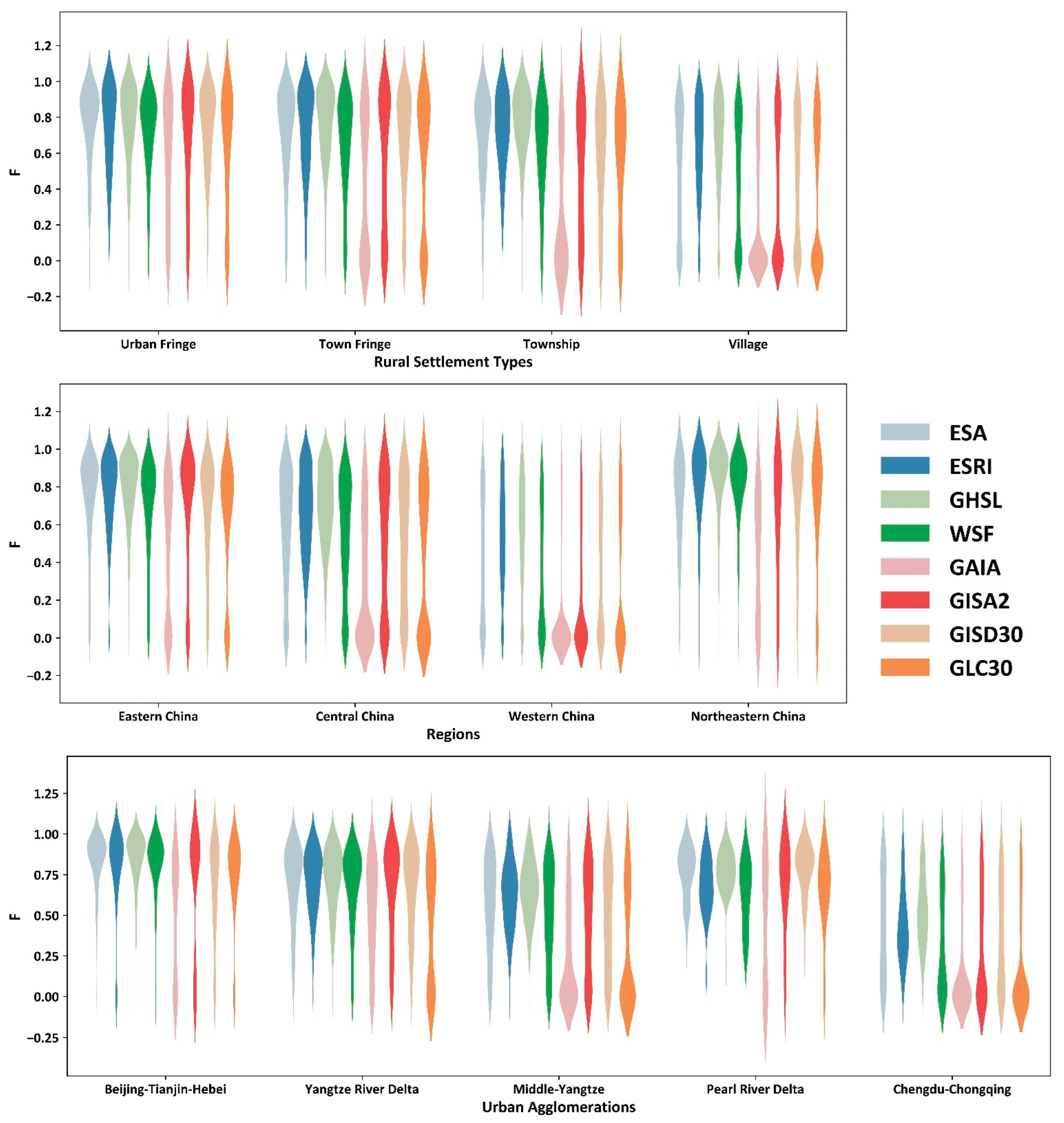
5.2.3. Pixel-Based Accuracy Test

Four accuracy indicators were calculated to reflect the overall accuracy by averaging the result of each error matrix in rural settlement units.

Table 4. The four overall accuracy indicators of the eight LULC maps.

		Overall Accuracy	Producer’s Accuracy	User’s Accuracy	F-score
10 m Resolution	ESA	0.851 (0.846)	0.505 (0.560)	0.764 (0.847)	0.566 (0.627)
	ESRI	0.765 (0.760)	0.896 (0.937)	0.538 (0.564)	0.636 (0.666)
	GHSL *	0.836 (0.833)	0.806 (0.840)	0.663 (0.659)	0.669 (0.697)
	WSF	0.836 (0.825)	0.428 (0.503)	0.790 (0.928)	0.511 (0.600)
30 m Resolution	GAIA	0.756 (0.736)	0.272 (0.539)	0.411 (0.813)	0.297 (0.586)
	GISA2.0	0.818 (0.823)	0.405 (0.588)	0.588 (0.853)	0.438 (0.637)
	GISD30	0.831 (0.820)	0.457 (0.538)	0.705 (0.830)	0.504 (0.593)
	GLC30	0.805 (0.718)	0.475 (0.754)	0.452 (0.718)	0.445 (0.707)

* The rural settlement pixels in the GHSL were extracted at a threshold value of 10%.

presents the results. The numbers without parentheses were generated with all of the VSUs. In general, the ranks and overall trends of the indicators were consistent with the omission results. The GHSL ranks first of the F-scores (0.669), with a relative balance between the PA (0.806) and UA (0.663). The ESRI ranks second in the F-scores (0.636) and benefitted greatly from having the highest producer’s accuracy (0.896), which indicates that it rarely missed real rural settlement pixels. However, a relatively high OA usually corresponds to a low UA. A typical example is the ESRI, whose UA value equals 0.538, even lower than the maps at 30 m resolution (GISA2.0 and GISD30). The ESA, WSF, and GISD30 roughly belonged to the same type in terms of PA (0.428–0.505), UA (0.705–0.790), and F-score (0.504–0.566). Among them, the UA of the WSF was the highest (0.79), reflecting that the rural settlement pixels of the WSF were more reliable than those of the other two maps.

The numbers in parentheses refer to the indicators calculated without the omitted VSUs. This result reflects the detection ability of the maps under scenarios that do not consider omissions, such as tracking the area changes of selected rural settlements [60]. The OAs of seven of the LULC maps (excluding the GISA2.0) became lower than those calculated with all VSUs. This is because the true negative (TN) pixels of the omitted USVs can still provide a high OA. From the F-score, there is no significant difference in the comprehensive accuracy of the eight LULC maps without omissions. The lowest was 0.589 (GAIA) and the highest was 0.707 (GLC30). Meanwhile, apart from the GHSL and ESRI, the maps had a low PA along with a high UA.

We examined the numerical distribution of the F-score through violin plots (see Figure 7) to determine the best LULC map for portraying rural settlements by type and region. A probability density function (PDF) was generated to show the distribution of the number of VSUs. For each violin, a higher center of gravity indicates a higher accuracy; a wider PDF suggests more concentrated values. The distributions of the F-score further confirm our findings. Four maps at 10 m resolutions present similar patterns in the city fringe, town fringe, and township, but the PDFs of the four maps at 30 m resolutions decline from city fringes to villages. No map has a concentrated PDF with a high F-score in the category of villages. Violin plots of the Western China and Chengdu–Chongqing urban agglomerations suggest poor performances of the maps. In Eastern, Central, and Northeastern China, the GHSL has the most centralized high PDF, followed by the ESA, WSF, and ESRI. The GISD30 performs as well as 10 m resolution maps in East China and Northeast China and ranks first place in the Pearl River Delta urban agglomeration.

6. Discussion

Some issues need to be further discussed to help better understand the accuracy of the products in their mapping of rural settlements.

6.1. Map Resolution

Maps at 10 m resolutions outperformed those at 30 m resolution. Given that the scale of a single building is roughly dozens of meters large [17,18] and the houses in the rural areas are usually small, it is easier to detect the presence of tiny villages for maps at 10 m resolutions. One exception is the ESRI, which had an excellent capability to detect rural settlements while neglecting the outlines of individual buildings. The product might be applicable for rural studies that do not involve area measurement and building contours. Small villages may be difficult to detect in 30 m resolution products due to the influence of mixed pixels.

6.2. Type of Rural Settlements

Practically, the functional characteristics of the maps should be considered when their accuracy is similar. The four maps with 10 m resolutions were sensitive to the development level of areas. If the target rural settlements located in city fringe, town fringe, or township were developed, the ESA, WSF, and GHSL may provide satisfactory performances in obtaining their boundary or area. The performances of all maps dramatically decreased in villages, probably because the training datasets of these maps were mainly extracted from urban areas and few were obtained from rural areas. Only the GHSL could strike a reasonable compromise between area and omission rate, which has made substantial improvements when compared with its early version at the 30 m resolution [19,36]. Hence, the GHSL is the best choice for studying small villages.

6.3. Spatial Variation across Regions

The ability to detect rural settlements in Eastern and Western China significantly differed, most likely due to the climate type, topography, architectural style, and economic development. However, many rural settlements with similar characteristics in scale, terrain, elevation, and architectural style were more accurately detected in Eastern China than in the west. This is more apparent for maps with 30 m resolutions. The performances of LULC products based on urban agglomerations were consistent with the results of regions, but the discrepancies among maps were more pronounced. For instance, the Chengdu–Chongqing urban agglomeration was better served by the GHSL, while the GISD30 better portrayed the Pearl River Delta urban agglomeration. Therefore, more exploration of the potential factors behind spatial heterogeneity is desirable to improve the ability of mapping rural settlements.

6.4. Balance between PA and UA

The F-score was employed in this paper to measure the comprehensive accuracy. Where there is little difference in the F-Score, PA and UA can reflect the functional tendency of the LULC maps, which can make a more detailed division of the application scenarios. For instance, the ESRI with its high PA overestimates the area of rural settlements because the ESRI typically covers small buildings with larger patches. The WSF with larger UA values can accurately depict building contours and may be suitable for drawing rural house layers.

6.5. Rural Roads

Both the ESA and WSF use optical and radar images, which exhibited similar effects and consistent trends in most situations. However, the WSF always tended to underestimate the area of rural settlements. The reason could be that the WSF only preserved buildings, whereas the VSUs treat roads as part of the rural settlements. The ESA detected impervious roads inside rural settlements and independent arterial roads outside of the rural settlements. The ESRI could detect roads when they were connected near buildings. The GHSL, with a lower threshold value, could more effectively distinguish rural roads. Among the maps at 30 m resolutions, the GAIA, GISD30, and GISA2.0 products could only identify wide impervious roads in urban areas, and the GLC30 could not identify any types of roads.

6.6. The Continuous Value of Built-Up Probability

Among the eight LULC maps, only the GHSL provides a continuous value to represent the proportion of built-up area in the mixed pixels. It allows users to flexibly detect rural settlements by determining the threshold value. For example, a slight increase in threshold value can improve the capture ability for detecting small built-up areas and reducing the omission rate. If we remove roads by setting a high threshold value, it is difficult to detect small settlements. However, the extent to which the threshold value has influence on the extraction of rural roads still needs to be tested.

6.7. Pixel Values of the Built Year

The development and evolution of rural settlements are important topics in rural research. The GAIA, GISD30, and GISA2.0 products take the year of the built-up area as a pixel value (as early as 1972, GISA2.0). The expansion process of cities or villages can be captured by multi-year layers. Although the comprehensive accuracy of these maps is not as good as that of 10 m resolution LULC maps, the GISD30 and GISA2.0 can also be used in many rural areas, particularly closer to cities in Eastern China or Northeastern China, notably in Pearl River Delta urban agglomeration.

7. Conclusions

This study selected eight of the latest LULC datasets to compare their accuracy for rural settlement detection using China as the study area. We created 2376 validation sample sites through the SSS method and conducted omission tests, area comparisons, and pixel-based accuracy tests. The results show that the maps at 10 m resolution are more precise than those at 30 m resolution; the GHSL has the highest comprehensive accuracy in various scenarios and one can flexibly adjust the threshold value to find a proper range of rural settlement size; the ESRI outperforms the other maps in detecting the existence of rural settlements, but it dramatically overestimates the area; the GISD30 performs best among maps with 30 m resolutions, notably in the Pearl River Delta urban agglomeration; villages in Western China remains a big challenge for all maps.

Table 5. Wise-use recommendations for LULC maps under different scenarios.

Map Quality	Description	Recommended Maps
Most Recent Map	The maps are recent.	ESRI provides global maps from 2015 to 2021, updated annually. ESA and GISD30 offer versions for 2020.
Long Time Coverage	Aggregating the built-up year on one map as pixel values.	GISD30 published a time-aggregated map for 1985–2020. GISA2.0 provides maps of earlier dates (1972–2019) but is inferior to GISD30 in all aspects.
Highest Comprehensive Map Accuracy	Strong agreement with the VSUs, providing the best balance of PA and UA.	GHSL is capable of mapping as many rural settlements as possible while simultaneously providing a high likelihood that the pixels obtained are rural settlements.
Highest Producer’s Accuracy (PA)	As many as rural settlements detected	ESRI can cover the most extensive rural settlement pixels. GHSL with a low threshold (e.g., 10%) follows ESRI closely.
Highest User’s Accuracy (UA)	Less false positives.	WSF has the highest UA regardless of the omission rate. ESA ranks second in UA, but its PA is higher than that of WSF.
Best for Estimating Area	Capability to estimate the area of a rural settlement.	ESA estimates area accurately in city fringes, town fringes, and township areas. GHSL with a low threshold value is suitable for estimating the area of small rural settlements of less than 5 hectares. WSF is the most accurate product in estimating the area of buildings.
Low Omission Rate	Fewer rural settlements ignored	ESRI (globally optimal) has the lowest omission rates in all rural settlement types. GHSL (locally optimal) has the lowest omission rates (all less than 1%) in 5 urban agglomerations and three regions (excluding Western China).
Roads	Including roads	GHSL can capture finer concrete paths. ESA only detects wide arterials.
	Excluding roads	WSF only depicts the presence of buildings and completely removes any roads between buildings.
Functional Types	High accuracy in the city fringes, town fringes, or townships (relatively developed rural settlements)	GHSL performs best, followed by ESRI, ESA, and WSF. GISD30 can support rural settlements in city fringes.
	High accuracy in villages (relatively less developed rural settlements)	GHSL is the only map used for pixel-scale analysis; other maps should consider omission rates across regions.

presents the recommended maps for various scenarios.

The results of this study indicate that there was spatial heterogeneity in the accuracy of mapping rural settlements. However, we only used China as the study area because of the availability of data; if more detailed information on villages from other countries is available, the ability of the maps to detect rural settlements can be further explored.

References

1. United Nations, Department of Economic and Social Affairs. World Urbanization Prospects: 2018 Revision; UN DESA: New York, NY, USA, 2018. [Google Scholar]
2. Brüntrup, M.; Messner, D. Global Trends and the Future of Rural Areas. Agric. Rural Dev. 2007, 1, 48–51. [Google Scholar]
3. United Nations. Transforming Our World: The 2030 Agenda for Sustainable Development; United Nations: New York, NY, USA, 2015. [Google Scholar]
4. Tian, Y.; Kong, X.; Liu, Y. Combining Weighted Daily Life Circles and Land Suitability for Rural Settlement Reconstruction. Habitat Int. 2018, 76, 1–9. [Google Scholar] [CrossRef]
5. Guo, K.; Huang, Y.; Chen, D. Analysis of the Expansion Characteristics of Rural Settlements Based on Scale Growth Function in Himalayan Region. Land 2022, 11, 450. [Google Scholar] [CrossRef]
6. Tan, M.; Li, X. The Changing Settlements in Rural Areas under Urban Pressure in China: Patterns, Driving Forces and Policy Implications. Landsc. Urban Plan. 2013, 120, 170–177. [Google Scholar] [CrossRef]
7. Chen, Z.; Liu, Y.; Feng, W.; Li, Y.; Li, L. Study on Spatial Tropism Distribution of Rural Settlements in the Loess Hilly and Gully Region Based on Natural Factors and Traffic Accessibility. J. Rural Stud. 2019, 93, 441–448. [Google Scholar] [CrossRef]
8. Song, W.; Li, H. Spatial Pattern Evolution of Rural Settlements from 1961 to 2030 in Tongzhou District, China. Land Use Policy 2020, 99, 105044. [Google Scholar] [CrossRef]
9. Gorbenkova, E.; Shcherbina, E. Historical-Genetic Features in Rural Settlement System: A Case Study from Mogilev District (Mogilev Oblast, Belarus). Land 2020, 9, 165. [Google Scholar] [CrossRef]
10. Song, W.; Liu, M. Assessment of Decoupling between Rural Settlement Area and Rural Population in China. Land Use Policy 2014, 39, 331–341. [Google Scholar] [CrossRef]
11. CIESIN (Center for International Earth Science Information Network). Global Rural-Urban Mapping Project (GRUMP) Alpha Version; NASA Socioeconomic Data and Applications Center (SEDAC): Palisades, NY, USA, 2004.
12. Schneider, A.; Friedl, M.A.; Potere, D. A New Map of Global Urban Extent from MODIS Satellite Data. Environ. Res. Lett. 2009, 4, 044003. [Google Scholar] [CrossRef]
13. Schneider, A.; Friedl, M.A.; Potere, D. Mapping Global Urban Areas Using MODIS 500-m Data: New Methods and Datasets Based on ‘Urban Ecoregions’. Remote Sens. Environ. 2010, 114, 1733–1746. [Google Scholar] [CrossRef]
14. European Space Agency. Land Cover CCI Product User Guide Version 2.0.; ESA: Paris, France, 2017. [Google Scholar]
15. Arino, O.; Gross, D.; Ranera, F.; Leroy, M.; Bicheron, P.; Brockman, C.; Defourny, P.; Vancutsem, C.; Achard, F.; Durieux, L.; et al. GlobCover: ESA Service for Global Land Cover from MERIS. In Proceedings of the 2007 IEEE International Geoscience and Remote Sensing Symposium, Barcelona, Spain, 23–28 July 2007; pp. 2412–2415. [Google Scholar] [CrossRef]
16. Sulla-Menashe, D.; Friedl, M.A. User Guide to Collection 6 MODIS Land Cover (MCD12Q1 and MCD12C1) Product; USGS: Reston, VA, USA, 2018. [CrossRef]
17. Potere, D.; Schneider, A.; Angel, S.; Civco, D.L. Mapping Urban Areas on a Global Scale: Which of the Eight Maps Now Available Is More Accurate? Int. J. Remote Sens. 2009, 30, 6531–6558. [Google Scholar] [CrossRef]
18. Klotz, M.; Kemper, T.; Geiß, C.; Esch, T.; Taubenböck, H. How Good Is the Map? A Multi-Scale Cross-Comparison Framework for Global Settlement Layers: Evidence from Central Europe. Remote Sens. Environ. 2016, 178, 191–212. [Google Scholar] [CrossRef]
19. Marconcini, M.; Metz-Marconcini, A.; Üreyen, S.; Palacios-Lopez, D.; Hanke, W.; Bachofer, F.; Zeidler, J.; Esch, T.; Gorelick, N.; Kakarla, A.; et al. Outlining Where Humans Live, the World Settlement Footprint 2015. Sci. Data 2020, 7, 242. [Google Scholar] [CrossRef]
20. Esch, T.; Heldens, W.; Hirner, A.; Keil, M.; Marconcini, M.; Roth, A.; Zeidler, J.; Dech, S.; Strano, E. Breaking New Ground in Mapping Human Settlements from Space—The Global Urban Footprint. ISPRS J. Photogramm. Remote Sens. 2017, 134, 30–42. [Google Scholar] [CrossRef]
21. Gong, P.; Wang, J.; Yu, L.; Zhao, Y.; Zhao, Y.; Liang, L.; Niu, Z.; Huang, X.; Fu, H.; Liu, S.; et al. Finer Resolution Observation and Monitoring of Global Land Cover: First Mapping Results with Landsat TM and ETM+ Data. Int. J. Remote Sens. 2013, 34, 2607–2654. [Google Scholar] [CrossRef]
22. Zanaga, D.; Kerchove, R.; Van De Keersmaecker, W. ESA WorldCover 10 m 2020 V100. 2021. Available online: https://pure.iiasa.ac.at/id/eprint/17832/ (accessed on 12 August 2022).
23. Zhang, X.; Liu, L.; Zhao, T.; Gao, Y.; Chen, X.; Mi, J. GISD30: Global 30-m Impervious Surface Dynamic Dataset from 1985 to 2020 Using Time-Series Landsat Imagery on the Google Earth Engine Platform. Earth Syst. Sci. Data Discuss. 2022, 14, 1831–1856. [Google Scholar] [CrossRef]
24. Huang, X.; Li, J.; Yang, J.; Zhang, Z.; Li, D.; Liu, X. 30 m Global Impervious Surface Area Dynamics and Urban Expansion Pattern Observed by Landsat Satellites: From 1972 to 2019. Sci. China Earth Sci. 2021, 64, 1922–1933. [Google Scholar] [CrossRef]
25. Gong, P.; Li, X.; Wang, J.; Bai, Y.; Chen, B.; Hu, T.; Liu, X.; Xu, B.; Yang, J.; Zhang, W.; et al. Annual Maps of Global Artificial Impervious Area (GAIA) between 1985 and 2018. Remote Sens. Environ. 2020, 236, 111510. [Google Scholar] [CrossRef]
26. De Colstoun, E.C.B.; Huang, C.; Wang, P.; Tilton, J.C.; Tan, B.; Phillips, J.; Niemczura, S.; Ling, P.-Y.; Wolfe, R. Documentation for the Global Man-Made Impervious Surface (GMIS) Dataset from Landsat; NASA Socioeconomic Data and Applications Center: Palisades, NY, USA, 2017.
27. Jun, C.; Ban, Y.; Li, S. Open Access to Earth Land-Cover Map. Nature 2014, 514, 434. [Google Scholar] [CrossRef]
28. Karra, K.; Kontgis, C.; Statman-Weil, Z.; Mazzariello, J.C.; Mathis, M.; Brumby, S.P. Global land use/land cover with Sentinel 2 and deep learning. In Proceedings of the 2021 IEEE International Geoscience and Remote Sensing Symposium IGARSS, Brussels, Belgium, 11–16 July 2021; pp. 4704–4707. [Google Scholar] [CrossRef]
29. Corbane, C.; Syrris, V.; Sabo, F.; Politis, P.; Melchiorri, M.; Pesaresi, M.; Soille, P.; Kemper, T. Convolutional Neural Networks for Global Human Settlements Mapping from Sentinel-2 Satellite Imagery. Neural Comput. Appl. 2021, 33, 6697–6720. [Google Scholar] [CrossRef]
30. Im, J.; Lu, Z.; Rhee, J.; Quackenbush, L.J. Impervious Surface Quantification Using a Synthesis of Artificial Immune Networks and Decision/Regression Trees from Multi-Sensor Data. Remote Sens. Environ. 2012, 117, 102–113. [Google Scholar] [CrossRef]
31. Zhou, Y.; Wang, Y.Q. Extraction of Impervious Surface Areas from High Spatial Resolution Imagery by Multiple Agent Segmentation and Classification. Photogramm. Eng. Remote Sens. 2008, 74, 857–868. [Google Scholar] [CrossRef]
32. Jensen, J.R.; Cowen, D.C. Remote Sensing of Urban/Suburban Infrastructure and Socio-Economic Attributes. Photogramm. Eng. Remote Sens. 1999, 65, 611–622. [Google Scholar]
33. Wang, Y.; Li, M. Urban Impervious Surface Detection From Remote Sensing Images: A Review of the Methods and Challenges. IEEE Geosci. Remote Sens. Mag. 2019, 7, 64–93. [Google Scholar] [CrossRef]
34. Jia, Y.; Tang, L.; Wang, L. Influence of Ecological Factors on Estimation of Impervious Surface Area Using Landsat 8 Imagery. Remote Sens. 2017, 9, 751. [Google Scholar] [CrossRef]
35. Sun, G.; Chen, X.; Ren, J.; Zhang, A.; Jia, X. Stratified Spectral Mixture Analysis of Medium Resolution Imagery for Impervious Surface Mapping. Int. J. Appl. Earth Obs. Geoinf. 2017, 60, 38–48. [Google Scholar] [CrossRef]
36. Mück, M.; Klotz, M.; Taubenbock, H. Validation of the DLR Global Urban Footprint in Rural Areas: A Case Study for Burkina Faso. In Proceedings of the 2017 Joint Urban Remote Sensing Event (JURSE), Dubai, United Arab Emirates, 6–8 March 2017; pp. 6–9. [Google Scholar] [CrossRef]
37. Conrad, C.; Rudloff, M.; Abdullaev, I.; Thiel, M.; Löw, F.; Lamers, J.P.A. Measuring Rural Settlement Expansion in Uzbekistan Using Remote Sensing to Support Spatial Planning. Appl. Geogr. 2015, 62, 29–43. [Google Scholar] [CrossRef]
38. Zheng, X.; Wu, B.; Weston, M.V.; Zhang, J.; Gan, M.; Zhu, J.; Deng, J.; Wang, K.; Teng, L. Rural Settlement Subdivision by Using Landscape Metrics as Spatial Contextual Information. Remote Sens. 2017, 9, 486. [Google Scholar] [CrossRef]
39. Ji, H.; Li, X.; Wei, X.; Liu, W.; Zhang, L.; Wang, L. Mapping 10-m Resolution Rural Settlements Using Multi-Source Remote Sensing Datasets with the Google Earth Engine Platform. Remote Sens. 2020, 12, 2832. [Google Scholar] [CrossRef]
40. Chen, Y.; Ge, Y. Spatial Point Pattern Analysis on the Villages in China’s Poverty-Stricken Areas. Procedia Environ. Sci. 2015, 27, 98–105. [Google Scholar] [CrossRef]
41. National Bureau of Statistics of China. Announcement on Updating National Statistical Code for Zoning and Code for Urban-Rural Division. Available online: http://www.stats.gov.cn/tjsj/tjbz/tjyqhdmhcxhfdm/2021/index.html (accessed on 12 August 2022).
42. National Bureau of Statistics of China. Rules for Compiling Zoning Codes and Urban-Rural Division Codes for Statistics. Available online: http://www.stats.gov.cn/tjsj/tjbz/200911/t20091125_8667.html (accessed on 12 August 2022).
43. Wang, P.; Huang, C.; Brown de Colstoun, E.C.; Tilton, J.C.; Tan, B. Global Human Built-up And Settlement Extent (HBASE) Dataset from Landsat; NASA Socioeconomic Data and Applications Center (SEDAC): Palisades, NY, USA, 2017.
44. Chen, B.; Xu, B.; Zhu, Z.; Yuan, C.; Suen, H.P.; Guo, J.; Xu, N.; Li, W.; Zhao, Y.; Yang, J. Stable Classification with Limited Sample: Transferring a 30-m Resolution Sample Set Collected in 2015 to Mapping 10-m Resolution Global Land Cover in 2017. Sci. Bull. 2019, 64, 370–373. [Google Scholar]
45. Liu, X.; Huang, Y.; Xu, X.; Li, X.; Li, X.; Ciais, P.; Lin, P.; Gong, K.; Ziegler, A.D.; Chen, A. High-Spatiotemporal-Resolution Mapping of Global Urban Change from 1985 to 2015. Nat. Sustain. 2020, 3, 564–570. [Google Scholar] [CrossRef]
46. Huang, X.; Huang, J.; Wen, D.; Li, J. An Updated MODIS Global Urban Extent Product (MGUP) from 2001 to 2018 Based on an Automated Mapping Approach. Int. J. Appl. Earth Obs. Geoinf. 2021, 95, 102255. [Google Scholar] [CrossRef]
47. Corbane, C.; Sabo, F.; Politis, P.; Vasileos, S. GHS-BUILT-S2 R2020A: Built-up Grid Derived from Sentinel-2 Global Image Composite for Reference Year 2018 Using Convolutional Neural Networks (GHS-S2Net); European Commission, Joint Research Centre (JRC): Brussels, Belgium, 2020. [Google Scholar]
48. Clark, M.L.; Aide, T.M.; Grau, H.R.; Riner, G. A Scalable Approach to Mapping Annual Land Cover at 250 m Using MODIS Time Series Data: A Case Study in the Dry Chaco Ecoregion of South America. Remote Sens. Environ. 2010, 114, 2816–2832. [Google Scholar] [CrossRef]
49. Yang, Y.; Xiao, P.; Feng, X.; Li, H. Accuracy Assessment of Seven Global Land Cover Datasets over China. ISPRS J. Photogramm. Remote Sens. 2017, 125, 156–173. [Google Scholar] [CrossRef]
50. Li, B.Y.; Pan, B.; Cheng, W.; Han, J.; Qi, D.; Zhu, C. Research on Geomorphological Regionalization of China. Acta Geogr. Sin. 2013, 68, 291–306. [Google Scholar]
51. Reuter, H.I.; Nelson, A.; Jarvis, A. An Evaluation of Void-filling Interpolation Methods for SRTM Data. Int. J. Geogr. Inf. Sci. 2007, 21, 983–1008. [Google Scholar] [CrossRef]
52. Shi, Z.; Ma, L.; Zhang, W.; Gong, M. Differentiation and Correlation of Spatial Pattern and Multifunction in Rural Settlements Considering Topographic Gradients: Evidence from Loess Hilly Region, China. J. Environ. Manag. 2022, 315, 115127. [Google Scholar] [CrossRef] [PubMed]
53. Seymour, L. Spatial Data Analysis: Theory and Practice; Cambridge University Press: Cambridge, UK, 2005; Volume 100, ISBN 9780511049866. [Google Scholar]
54. Dunn, R.; Harrison, A.R. Two-Dimensional Systematic Sampling of Land Use. J. R. Stat. Soc. Ser. C Appl. Stat. 1993, 42, 585–601. [Google Scholar] [CrossRef]
55. Tian, G.; Qiao, Z.; Zhang, Y. The Investigation of Relationship between Rural Settlement Density, Size, Spatial Distribution and Its Geophysical Parameters of China Using Landsat TM Images. Ecol. Model. 2012, 231, 25–36. [Google Scholar] [CrossRef]
56. Mathew, O.O.; Sola, A.F.; Oladiran, B.H.; Amos, A.A. Efficiency of Neyman Allocation Procedure over Other Allocation Procedures in Stratified Random Sampling. Am. J. Theor. Appl. Stat. 2013, 2, 122–127. [Google Scholar] [CrossRef]
57. National Bureau of Statistics of China. Statistical Communiqué of the People’s Republic of China on the 2021 National Economic and Social Development; NBS: Beijing, China, 2022.
58. Fang, C. Important Progress and Future Direction of Studies on China’s Urban Agglomerations. J. Geogr. Sci. 2015, 25, 1003–1024. [Google Scholar] [CrossRef]
59. Foody, G.M. What Is the Difference between Two Maps? A Remote Senser’s View. J. Geogr. Syst. 2006, 8, 119–130. [Google Scholar] [CrossRef]
60. İzgi, B.D. Resilience of Rural Settlement Morphology Dynamics: The Case of Kargalı District (Village). J. Des. Resil. Arch. Plan. 2022, 3, 112–126. [Google Scholar]
Figure 1. Study area and rural settlements. (a) Longzhen; (b) Nangou; (c) Fanhuxi; (d) Langsha; (e) Chongji.
Land 11 01308 g001
Figure 2. Example of a validation sample unit.
Land 11 01308 g002
Figure 3. Stratification regions and sample rural settlements.
Land 11 01308 g003
Figure 4. Area test results of the four types of rural settlements. (a) ESA; (b) ESRI; (c) GHSL; (d) WSF; (e) GAIA; (f) GISA2.0; (g) GISD30; (h) GLC30.
Land 11 01308 g004
Figure 5. Area test results of four regions in China. (a) ESA; (b) ESRI; (c) GHSL; (d) WSF; (e) GAIA; (f) GISA2.0; (g) GISD30; (h) GLC30.
Land 11 01308 g005
Figure 6. Area test results of five urban agglomerations in China. (a) ESA; (b) ESRI; (c) GHSL; (d) WSF; (e) GAIA; (f) GISA2.0; (g) GISD30; (h) GLC30.
Land 11 01308 g006
Figure 7. The violin plot of the F-score for the eight LULC maps tested.
Land 11 01308 g007