Ecosystem and Driving Force Evaluation of Northeast Forest Belt

Abstract

The ecosystem in the Northeast Forest Belt (NFB) can provide various ecosystem services, such as soil conservation, habitat provision, water conservation, and so on. It is essential for maintaining the ecological environment in Northeast China and the entire country. In the face of increasingly severe environmental problems, the comprehensive and accurate evaluation of ecosystem conditions and their changes is significant for scientific and reasonable recovery and protection measures. In this study, the NFB was taken as the research area. The spatio-temporal changes in ecological quality from 2005 to 2015 and the main driving factors behind them were analyzed by constructing the comprehensive ecosystem evaluation index. The results showed that: The landscape types of the NFB were mainly forest, cropland, and grassland. And the better ecological environment of the NFB was mainly distributed in the south of Changbai Mountains (CBM), the middle of Lesser Khingan Mountains (LKM), and the northwest of Greater Khingan Mountains (GKM). In contrast, the northeast of CBM, the southwest of LKM, and the edge of southern GKM were relatively poor. During 2005–2015, the ecosystem in the NFB was in a relatively good state as a whole, showing a steady-to-good development trend. However, more attention needed to be paid to some areas where degradation still existed. Land use/cover, climate (annual average rainfall, etc.), and human disturbance were potential factors affecting ecosystem evolution in the NFB. This study aims to provide an effective scientific basis and policy reference for the environmental protection and construction of the NFB.

1. Introduction

As the largest ecosystem on land, the forest ecosystem can provide a variety of ecosystem services (ES) such as soil conservation service (SCS), carbon sequestration service (C), habitat provision service (HP), sand-stabilization service (SSS), water conservation service (WCS) and so on. The Northeast Forest Belt (NFB) contains China’s typical and essential forest ecosystem [1]. Due to the rich forest and biological resources, it is an important forest resource and biodiversity protection base in China. At the same time, because of the fertile soil and rich mineral resources, the NFB is an important food base and an old industrial base in China. To further protect the environment and promote regional sustainable development, China proposed the strategic pattern of building “two ecological barriers and three shelters” ecological stability in 2006 [2].

However, under the dual influence of global climate change and human disturbance, a series of ecological environment problems have been triggered, affecting the ecological environment stability in Northeast China. Understanding ecosystem evolution and driving factors is significant for ecosystem protection and sustainable development [3,4,5,6,7,8,9,10]. In the face of increasingly serious ecological problems, it is urgent to scientifically evaluate the ecosystem status, changing trends, and driving factors of the NFB. With the construction of the pattern of “two ecological barriers and three shelters” in China, many studies of the ecosystem of the NFB have also been carried out. Sun [1] assessed the ecosystem pattern, quality, and service function of the NFB by remote sensing data combined with monitoring statistical data through model simulation and sample surveys, and analyzed the changing trend between 2000 and 2010. It was found that there was no significant change in ecosystem quality (EQ) and service function of the NFB during the period. Still, the interference of social activity factors was increasing continuously. Based on this study, the calculation model of net ecosystem production was constructed to evaluate the carbon sequestration in the forest ecosystem of NFB [2]. It was concluded that the overall performance of carbon sequestration was carbon sinks, and human disturbances such as urban expansion, poor vegetation growth, and high temperature were significant factors affecting carbon sequestration. It provided an effective scientific basis for formulating ecological and environmental protection measures and policies in the NFB. After that, Su et al. [3] analyzed the changes in landscape pattern in the NFB from 2000 to 2015, and pointed out that the ecosystem in the NFB remained stable as a whole for 15 years, and simulated the changing trend in 2020. Qi et al. [11] explored the spatial differentiation characteristics and mechanism of trade-offs and synergies among six different ES in the NFB, indicating that the six ES showed a significant aggregation distribution, and the trade-offs and synergies had apparent spatial differentiation. Zhu et al. [12] evaluated the spatial-temporal distribution and changes in ecological vulnerability in the NFB in two different periods. They concluded that the overall ecological vulnerability was at a good level. Net primary productivity and land use types were the main driving factors affecting the spatial differentiation pattern of ecological vulnerability. This series of studies have provided a certain theoretical and scientific basis for the ecological system protection and management and its sustainable development in the NFB. However, previous studies have not constructed a comprehensive evaluation index for the NFB, so as to conduct a more integrated and comprehensive evaluation of its ecosystem.

Due to the limitations of single-factor evaluation results, more and more studies have begun to construct remote sensing ecological index (RSEI) to comprehensively evaluate and analyze the ecosystem changes in different regions [13,14,15,16]. In recent years, analyzing ecosystem evolution based on RSEI is also a hot topic worldwide. Mohammad et al. [17] used RSEI and impervious surface percentage feature space to map the urban surface ecological poorness zone (USEPZ) by combining land surface temperature (LST), humidity, normalized difference vegetation index (NDVI), and normalized difference soil index (NDSI), and thus proposed a new method for quantifying USEPZ. The results showed that the significant differences between surface ecological status (SES) and USEPZI in different cities were mainly caused by the physical characteristics of surface organisms. Based on this study, Mohammad et al. [18] continued to develop a new surface ecological condition index--land surface ecological status composition index (LSESCI) and compared it with RSEI. It was concluded that LSESCI was superior to RSEI in simulating the spatial and temporal changes of SES. At the same time, Karbalaei et al. [19] also synthesized RSEI under the PSR (pressure-state-response) framework by using principal component analysis combined with NDVI, LST, land surface moisture (LST) and normalized differential built-up, and bare soil index (NDBSI). The results showed that the disturbance of human activities and climate change disturbed the ecological balance, resulting in the reduction of urban EQ. Then based on RSEI, Maity et al. [20] used Landsat image data to evaluate the temporal and spatial variation of ecological environment quality in Kolkata urban agglomeration. The results accurately described the ecological environment quality of the study area, which could help the policy makers to scientifically guide ecological management decisions. In China, compared with other relevant studies, Xu et al. [21] early proposed a new remote sensing ecological index by coupling four evaluation indexes: vegetation index, surface temperature, humidity component, and soil index, and integrating each index with principal component transformation. Based on previous studies, the proposed remote sensing ecological index was improved, and the time series of ecological status images were generated by using the improved index and surface temperature images to realize the detection of ecological changes at different scales [22]. Then Yuan et al. [23] constructed remote sensing ecological index by integrating NDVI, humidity, LST, and NDBSI, and analyzed the temporal and spatial changes of EQ in Dongting Lake Basin from 2001 to 2019. Wang et al. [24] selected four indicators of humidity, greenness, dryness, and heat, and used the principal component analysis method to construct the ecological environment quality evaluation index. Combined with the land use data of Xinjiang and the central urban area of Urumqi, they explained the ecological environment quality and land use status in each period, thus revealing its dynamic development trend. Although the RSEI has high effectiveness and reliability and is widely used in different regions and ecosystem assessments, it ignores the impact of land use/ cover change on the structure and function of the ecosystem [23,25,26]. Single-factor (or specific-factor) assessments are oriented and can be used to assess ecosystem conditions from a specific perspective. Although multi-factor (pattern-quality-function) multi-level assessments can systematically and comprehensively assess ecosystems, the results of different levels of assessments have opposite conclusions among certain regions [27,28,29].

To sum up, using a comprehensive evaluation index to evaluate the changes in the ecosystem in each region effectively reduces the uncertainty based on single-factor evaluation results. In addition, combined with the analysis of various influencing factors, we can more comprehensively and accurately understand the impact of natural and human disturbance on the ecosystem. Therefore, this study used remote sensing (RS) and GIS technology, based on the “pattern-quality-service” evaluation framework system, using the analytic hierarchy process (AHP) to determine the weight of each index, and constructed a comprehensive index to evaluate the ecosystem of the NFB. The purpose of this study was: (1) To assess the long-term dynamic changes of EQ in the NFB from 2005 to 2015; (2) To explore the driving forces of these changes. This study can provide decision support and a scientific basis for the ecosystem stability of the NFB.

2. Materials and Methods

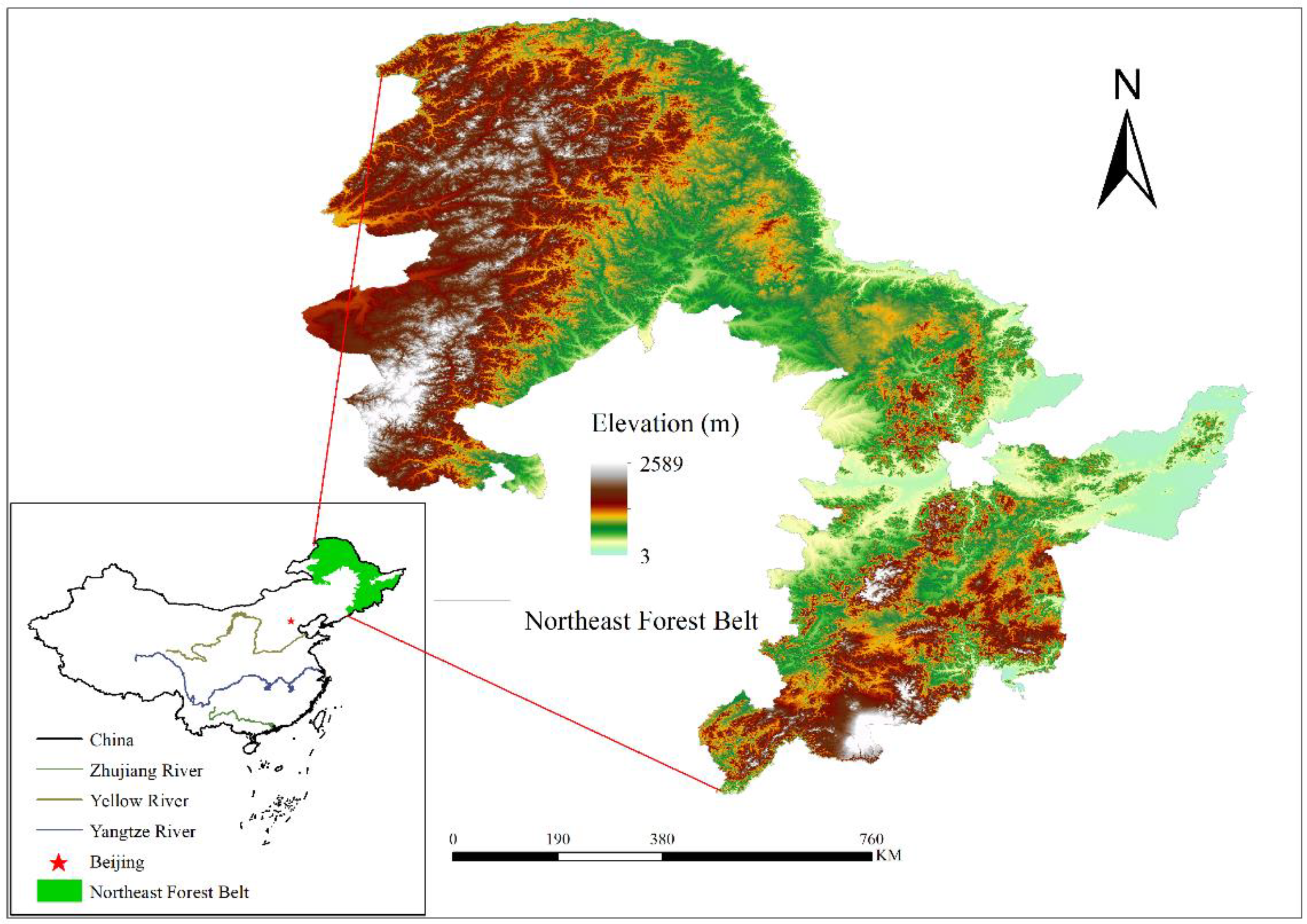
2.1. Study Area

The study area is located in the NFB. According to its geographical characteristics, it can be divided into three regions: Greater Khingan Mountains (GKM) area, Lesser Khingan Mountains (LKM) area, and Changbai Mountains (CBM) area. The NFB is located in 118°48′~134°22′ East longitude and 40°52′~53°34′ North latitude, with a total area of about 670,000 km², of which the forest area accounts for about 400,000 km². The terrain is diverse, mainly mountainous and hilly, the landscape is undulating, and the soil is fertile. The climate belongs to the temperate monsoon climate, hot and rainy in summer, dry and less rain in winter, and relatively cold; four seasons are distinct; annual precipitation is about 300~1000 mm. As the ecological stability barrier in Northeast China, the NFB is a forest region with a high conservation value in Northeast China [3,12]. The location of the study area is shown in Figure 1.

2.2. Data Source and Processing

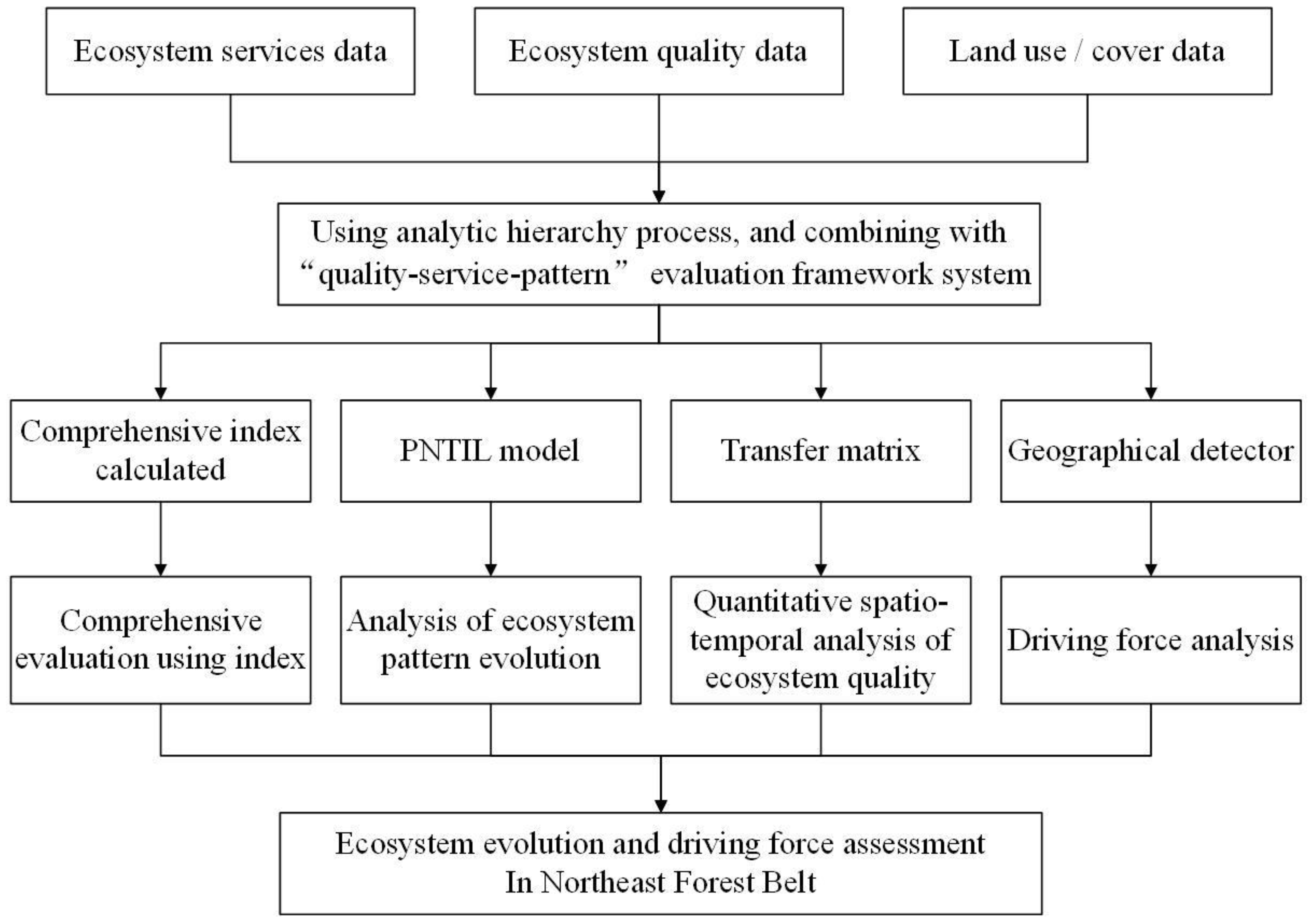
The DEM data used in this study is original elevation products with STRMDEM 90 m resolution, downloaded from the Geospatial Data Cloud Platform of the Computer Network Information Center of the Chinese Academy of Sciences (http://www.gscloud.cn) and accessed on 3 March 2022. The land use/cover data used are MODIS land use products from the NASA official website (https://ladsweb.nascom.nasa.gov/search), accessed on 3 March 2022. The soil data is derived from the harmonious world soil database China subset of the National Qinghai-Tibet Plateau/Third Pole Environmental Data Center, which includes soil texture, sandy soil, silt, clay, and organic carbon. Climate data comes from the National Meteorological Information Center (http://data.cma.cn) (accessed on 7 March 2022), which includes annual precipitation and temperature, relative humidity, sunshine hours, etc. The Data Centre for Resources and Environmental Sciences (RESDC) of the Chinese Academy of Sciences (http://www.resdc.cn) (accessed on 7 March 2022) provides population density and GDP data (spatial resolution 1 km). The road data used are downloaded on OpenStreetMap. The road type is national highway and expressway. To facilitate spatial analysis and comparison, all data used in this study is resampled to grid data with a 1 km resolution.

In this study, after completing the collection and pretreatment of various types of data, based on the “pattern-quality-service” evaluation framework system, the AHP was used to determine the weight coefficient of each index. Then ArcGIS was used to calculate the ecosystem comprehensive evaluation index, which was used to comprehensively evaluate the ecosystem evolution in the NFB. At the same time, the forward and reverse conversion index (PNTIL) model was used to analyze the evolution of its ecosystem pattern. The transfer matrix was used for quantitative spatio-temporal analysis of EQ, and the geographical detector model was used to analyze its driving force. The technical roadmap is shown in Figure 2.

2.3. Methods

2.3.1. Construction of Ecosystem Comprehensive Evaluation Index

Changes in land use patterns will directly affect the type and intensity of services provided by ecosystems. As the supply area of ES such as WCS, C, and HP, the introduction of ES accounting into land use decision-making in the NFB can better promote the rational development of natural resources and achieve sustainable land use. In addition, as an important part of the ecosystem, the in-depth assessment of the growth status and vitality of vegetation should also be an essential parameter for ecosystem assessment. Through the analysis of various influencing factors, the comprehensive evaluation index is used to evaluate the changes in the ecosystems in various regions, which can more comprehensively and accurately understand the influence of natural and human disturbance on the ecosystem. Therefore, this study used a “quality-service-pattern” assessment framework to evaluate the evolution and driving forces of the NFB ecosystems. Based on the ecosystem’s “quality-service-pattern” evaluation framework, a comprehensive index evaluation model (

Table 1. Comprehensive index evaluation model.

Goal Layer	Labeling Layer	Indicator Layer	Unit	Property	Weight
Comprehensive Index	Ecosystem service	SSS	t/(km2·a)	+	0.0337
		SCS	t/(km2·a)	+	0.0531
		WCS	t/(km2·a)	+	0.1415
		C	t/(km2·a)	+	0.2251
		HP	-	+	0.0867
	Ecosystem quality	FVC	%	+	0.1623
		NPP	gc/m2	+	0.0537
		LAI	-	+	0.0809
	Ecosystem pattern	LULC	-	+	0.1630

) was constructed. The indicators were calculated using remote sensing, land use, other data, and related ecological process models.

The weight coefficient was determined by the AHP [30,31,32]. The main steps of AHP were as follows: Firstly, the hierarchical model of the NFB ecosystem was established, which was divided into three levels, including goal layer A, labeling layer B, and indicator layer C. Secondly, seven experts in this study scale the factors at each level and constructed judgment matrix, that is, the number 1~5 and its reciprocal were used as the scale to objectively judge the factors of each level. Subsequently, the eigenvector and the maximum eigenvalue of the matrix were obtained, and the consistency test of the matrix was carried out to obtain the weight coefficients. In this study, CR < 0.1 passed the consistency test. The judgment matrix of different levels is shown in

Table 2. Judgment matrix of different levels.

Hierarchical Model	Judgment Matrix							Consistency Test
A–B	A	B1		B2	B3		Wi	CR = 0.052 λmax = 3.054
	B1	1		1/3	2		0.2969
	B2	3		1	3		0.5401
	B3	1/2		1/3	1		0.1630
B1–C	B1	C1		C2	C3		Wi	CR = 0.009 λmax = 3.009
	C1	1		3	2		0.5466
	C2	1/3		1	1/2		0.1810
	C3	1/2		2	1		0.2724
B2–C	B2	C4	C5	C6	C7	C8	Wi	CR = 0.015 λmax = 5.068
	C4	1	3	4	1/2	2	0.2620
	C5	1/3	1	2	1/4	1/4	0.0984
	C6	1/4	1/2	1	1/5	1/3	0.0623
	C7	2	4	5	1	3	0.4167
	C8	1/2	2	3	1/3	1	0.1606

Note: A is the goal layer; B is the labeling layer, and B1–B3 are ecosystem quality, ecosystem service, and ecosystem pattern; C is the indicator layer, C1–C8 are FVC, NPP, LAI, WCS, SCS, SSS, C, HP; Wi is the weight value.

. The consistency test index formulas are [33,34]:

$$CR=CI/RI$$

(1)

$$CI=\frac{{\lambda }_{\max }-n}{n-1}$$

(2)

where $CI$ is the deviation consistency index; $RI$ is the average consistency index; ${\lambda }_{\max }$ is the maximum eigenvalue; $n$ is the order of the judgment matrix; ensuring that the ratio of CI to RI is less than 0.1 [34].

Then the obtained weight coefficients are used to calculate the comprehensive index. The calculation method is [35]:

$$V_{cei}={{\displaystyle \sum }}_{i=1}^n{V}_i\times {\epsilon }_i$$

(3)

where, $V_{cei}$ is the composite index; $V_i$ is the evaluation result of indicator i; ${\epsilon }_i$ is the weight of the first index.

2.3.2. Ecosystem Service

One of the important purposes of the construction of the NFB is to improve regional ES and promote regional ecological stability. The rich ES assessment in the NFB is added to the assessment framework system, which can better realize the protection, improvement, and sustainable development of the ecosystem. Therefore, this study selected SSS, SCS, WCS, C, and HP five ES for analysis and evaluation.

SSS is usually estimated by the amount of sand-stabilization of vegetation. By calculating the difference between the potential and the actual wind erosion, the sand stabilization of vegetation can be estimated. The potential wind erosion refers to the wind erosion when there is no vegetation, and the actual wind erosion refers to the wind erosion when there is vegetation. The calculation formulas are [36]:

$$SR=S_{L1}-S_{L2}$$

(4)

$$S_{L1}=\frac{2 · x}{S_1{}^2}{Q}_{\max 1} · e^{-{\left(\frac{x}{S_1}\right)}^2}$$

(5)

$$S_{L2}=\frac{2 · x}{S_2{}^2}{Q}_{\max 2} · e^{-{\left(\frac{x}{S_2}\right)}^2}$$

(6)

$$Q_{\max 1}=109.8\left[WF\times EF\times SCF\times K^{\prime }\right]$$

(7)

$$S_1=150.71{\left(WF\times EF\times SCF\times K^{\prime }\right)}^{-0.3711}$$

(8)

$$Q_{\max 2}=109.8\left[WF\times EF\times SCF\times K^{\prime }\times COG\right]$$

(9)

$$S_2=150.71{\left(WF\times EF\times SCF\times K^{\prime }\times COG\right)}^{-0.3711}$$

(10)

where $SR$ is the sand-stabilization, kg/m²; $S_{L1}$ and $S_{L2}$ are potential wind erosion and actual wind erosion, kg/m², respectively; $Q_{\max 1}$ and $Q_{\max 2}$ are the maximum migration capacities of potential and actual soil erosion, kg/m; $S_1$ and $S_2$ are the critical field lengths of potential and actual soil erosion, respectively, m; $x$ is the maximum wind erosion distance, m; $WF$ is the meteorological factor; $EF$ is the soil erodibility factor; $SCF$ is a soil crust factor; $K^{\prime }$ is the surface roughness factor; $COG$ is the vegetation cover factor.

SCS is usually estimated by the soil conservation of vegetation. The soil conservation of vegetation can be estimated by calculating the difference between the potential and the actual soil conservation. The potential soil conservation refers to the amount of soil erosion generated without vegetation, and the actual soil conservation refers to the amount of soil erosion generated with vegetation. This study selected USLE to evaluate SCS in the NFB ecosystems. The calculation formula is as follows [37]:

$$SC=S{E}_p-S{E}_a=R · K · LS · \left(1-COG\right)$$

(11)

where, $SC$ is soil conservation, [t/(hm² a)]; $S{E}_p$ and $S{E}_a$ are potential and actual soil conservation, respectively, [t/(hm² a)]; $R$ is rainfall erosivity factor, MJ·mm/(hm²·ha); K is soil erodibility factor, t∙hm²∙h/(hm²∙MJ∙mm); $LS$ and $COG$ are terrain factor, vegetation cover factor, no dimension.

WCS is usually estimated by the water balance equation. WCS can be estimated using precipitation minus evaporation, evapotranspiration, and rainstorm runoff. The calculation formula is as follows [38]:

$$WR=PRE-ET-QF$$

(12)

where $WR$ is water conservation, mm; $PRE$ is annual precipitation, mm; $QF$ is rainstorm runoff, mm. $ET$ is the actual evaporation and emission, mm.

C is usually calculated using above-ground biomass multiplied by the biomass-carbon conversion coefficient. The main calculation formula is as follows [39]:

$$COS={\displaystyle \sum }_{i=1}^{j}AG{B}_i\times C_i$$

(13)

where $COS$ is the ecosystem carbon storage; $i$ is the type i ecosystem; $j$ is the total number of ecosystem types; $AG{B}_i$ is the above-ground biomass of ecosystem type i; $C_i$ is the biomass-carbon conversion coefficient of i ecosystem types.

HP is usually estimated by the distribution of indicator species in county units. The calculation formula is [11]:

$$E_{\mathrm{a}}={{\displaystyle \sum }}_{i=1}^n{E}_i$$

(14)

where $E_{\mathrm{a}}$ indicates the total number of species (number); $E_i$ is the number of species (number).

2.3.3. Ecosystem Quality

Vegetation is an important part of the ecosystem, which connects the natural processes such as the atmosphere, water, and soil. Its change will directly affect the regional climate, hydrology, and soil conditions, and has an important impact on the regional energy cycle and the biochemical cycle of substances. It is an important indicator of regional EQ change. It is also significant to add the in-depth evaluation of vegetation growth status and growth vigor into the evaluation framework system. Therefore, this study selected fractional vegetation coverage (FVC), net primary productivity (NPP), leaf area index (LAI), three EQ analyses, and evaluations.

FVC refers to the ratio of the vertical projection area of plants in a region to that of the region, which is one of the most essential indicators to measure EQ and surface vegetation status. Normally, the FVC is usually calculated by NDVI. The calculation formulas are [40]:

$$\mathrm{NDVI}=\left({\mathsf{\rho }}_{\mathrm{NIP}}-{\mathsf{\rho }}_{\mathrm{R}}\right)/\left({\mathsf{\rho }}_{\mathrm{NIP}}+{\mathsf{\rho }}_{\mathrm{R}}\right)$$

(15)

where ${\mathsf{\rho }}_{\mathrm{NIP}}$ and ${\mathsf{\rho }}_{\mathrm{R}}$ are the reflectivity of near-infrared band and red band, respectively.

$$\mathrm{FVC}=\left(\mathrm{NDVI}-{\mathrm{NDVI}}_{\mathrm{soil}}\right)/\left({\mathrm{NDVI}}_{\mathrm{veg}}-{\mathrm{NDVI}}_{\mathrm{soil}}\right)$$

(16)

where $\mathrm{FVC}$ is fractional vegetation coverage, ${\mathrm{NDVI}}_{\mathrm{veg}}$ is the NDVI value of pure vegetation pixel, and ${\mathrm{NDVI}}_{\mathrm{soil}}$ is the NDVI value of no vegetation pixel.

NPP reflects the efficiency of fixing and converting light energy into compounds in plants. NPP can well reflect the vegetation productivity and EQ. At present, there are many models to calculate NPP. In this study, the CASA model estimates the NPP of the NFB. In the CASA model, NPP is mainly determined by the two variables of APAR and light energy conversion rate (ε) absorbed by vegetation. The calculation formulas are [41]:

$$\mathrm{NPP}=\mathrm{APAR}\left(t\right)\times \epsilon \left(t\right)$$

(17)

$$\mathrm{APAR}=\mathrm{FPAR}\times \mathrm{PAR}$$

(18)

$$\epsilon \left(t\right)=\epsilon \times T1\left(t\right)\times T2\left(t\right)\times W\left(t\right)$$

(19)

where $\mathrm{APAR}\left(t\right)$ is the photosynthetically active radiation absorbed by plants; $\epsilon \left(t\right)$ is the conversion efficiency of APAR into organic carbon; $\mathrm{FPAR}$ is the effective absorptivity of APAR by plants; $\mathrm{PAR}$ is the driving energy of plant photosynthesis. $\epsilon$ is the maximum light energy conversion rate under ideal conditions; $T1\left(t\right)$ and $T2\left(t\right)$ are the effects of temperature and photosynthesis in varying degrees, respectively; $W\left(t\right)$ is the influence coefficient of water stress.

LAI refers to the ratio of the total leaf area of plants to the land area per unit of land area. LAI can reflect the vegetation growth in vertical structure, which is also one of the important indicators for evaluating EQ. There are many methods to calculate LAI, among which remote sensing technology can realize dynamic real-time and large-scale monitoring of LAI. The vegetation canopy radiative transfer model is one of the common models to calculate LAI by using remote sensing technology. The corresponding radiative transfer process is described as follows [42]:

$$-\mu \frac{\partial L(z,\Omega )}{\partial \tau }+G\left(\tau ,\Omega \right)L(z,\Omega )=\frac{\omega }{4\pi }\underset{4\pi }{\overset{}{{\displaystyle \int }}}p\left({\Omega }^{\prime }\to \Omega \right)G\left({\Omega }^{\prime }\right)L(z,{\Omega }^{\prime })d{\Omega }^{\prime }$$

(20)

where $L$ is brightness; $\mu =cos\theta$ is the chord value of transmission direction zenith angle; $G$ is the leaf angle distribution function; $\omega$ is the leaf albedo; $p\left({\Omega }^{\prime }\to \Omega \right)$ is the vegetation canopy phase function.

2.3.4. Evolution of Ecosystem Pattern

The land use/cover change has an important function in maintaining ecosystem service function. Land use/cover change will affect the function and structure of the ecosystem, and the evolution of land use/cover mode will directly affect the types and intensity of ES. It is significant to study the evolution of ecosystem service value driven by land use/cover change, which is also an essential quantitative index of environmental effects of land use/cover change. Therefore, this study selected the ecosystem transfer matrix and PNTIL model to analyze and evaluate the land use/cover change in the NFB.

The ecosystem transfer matrix can effectively list the conversion relationship between different ecosystems in different periods in the form of a matrix to reflect the change characteristics of ecosystems and the flow direction between systems in detail, and quantify the conversion status between systems [43,44,45,46]. Using the following formula to calculate the proportion of different types of landscape areas [47]:

$$P_{\mathit{ij}}=S_{\mathit{ij}}/TS\left(i=1,2,\dots ,n;j=1,2,\dots ,n\right)$$

(21)

where $P_{\mathit{ij}}$ is the area ratio of type i ecosystem based on classification at all levels in the first year of the ecosystem classification system; $S_{\mathit{ij}}$ is the area of category i ecosystems in the ecosystem classification system at all levels in the year j; $TS$ is the total area of the evaluation area; $n$ is the number of ecosystem types.

PNTIL model can analyze the evolution trend of ecosystem patterns [47,48,49]. Based on the stability and biodiversity of each ecosystem, the ecosystem transformation was divided into positive change and reverse change, and the positive/reverse transformation rules of the ecosystem were established (

Table 3. Rules of forward/reverse ecosystem transformation.

Ecosystem Type	Types after Conversion	Conversion Direction
Forest (I)	III	+
	II, IV, V, VI, VII	-
Grassland (II)	I, III	+
	IV, V, VI, VII	-
Wetland (III)	-	+
	I, II, IV, V, VI, VII	-
Cropland (IV)	I, II, III	+
	V, VI, VII	-
Built-up land (V)	I, II, III, IV	+
	VI, VII	-
Desert (VI)	I, II, III, IV, V, VII	+
	-	-
Others (VII)	I, II, III, IV, V	+
	VI	-

). The ecosystem transfer matrix of the NFB from 2005 to 2015 was used to quantitatively evaluate the ecosystem PNTIL of the NFB. The calculation formula of the ecosystem conversion index is [47]:

$$LCT{R}_{i,k}=\left(\Delta S_{i,k}/S_i\right)\times 1/t\times 100$$

(22)

where $LCT{R}_{i,k}$ is the conversion rate of ecosystem type to k in the i region; $S_i$ is the total area of all ecosystems in region i; $\Delta S_{i,k}$ is the total area converted into k type; k = 1 represents the positive conversion rate of ecosystems in the region; k = 2 represents the inverse conversion rate of the ecosystem, $t$ being a time variable.

2.3.5. Quantitative Spatio-Temporal Analysis of EQ

A quantitative spatio-temporal analysis of EQ in the NFB was carried out. The results of EQ were divided into five grades, and the transfer matrix of five grades of EQ in three periods was counted to reflect the changes in EQ in time and space. Using the following formula to calculate the proportion of different levels of EQ area [47]:

$$P_{\mathit{ij}}=S_{\mathit{ij}}/TS\left(i=1,2,\dots ,n;j=1,2,\dots ,n\right)$$

(23)

where $P_{\mathit{ij}}$ is the area ratio of type i EQ in year j based on classification at all levels in the EQ classification system; $S_{\mathit{ij}}$ is the area of category i EQ in year j based on classification at all levels in the EQ classification system; $TS$ is the total area of the evaluation area; $n$ is the number of types of EQ at different levels.

2.3.6. Ecosystem Driving Force Analysis

The geo-detector model is mainly a new statistical method to reveal the driving factors behind spatial differentiation, which can detect whether a certain factor is a reason for the evolution of the ecosystem. This model mainly uses the q-value measurement factor to detect the results. The larger the q-value, the stronger the driving effect of independent variables for the spatial differentiation of dependent variables and vice versa [50,51,52,53,54,55]. Based on the availability of relevant research [12,35] and regional data, 18 potential socio-ecological driving factors were selected as independent variables X. The comprehensive evaluation indexes of the ecosystem in the three periods of 2005, 2010, and 2015 were selected as the dependent variable Y, including terrain-related factors (elevation, slope, aspect), climate (annual average precipitation, annual average temperature), social economics (population density, GDP, road), and land cover (cropland, forest, grassland, wetland, built-up land, desert, other types), soil texture (silt, clay, sand). Next, the natural breakpoint method was used to change the independent variable X from numerical value to category quantity. The independent variable X was matched with the dependent variable Y. Then, the geographical detector model was used for factor detection analysis. Finally, the influence value and driving effect of each variable X for the dependent variable Y were obtained.

3. Results and Analysis

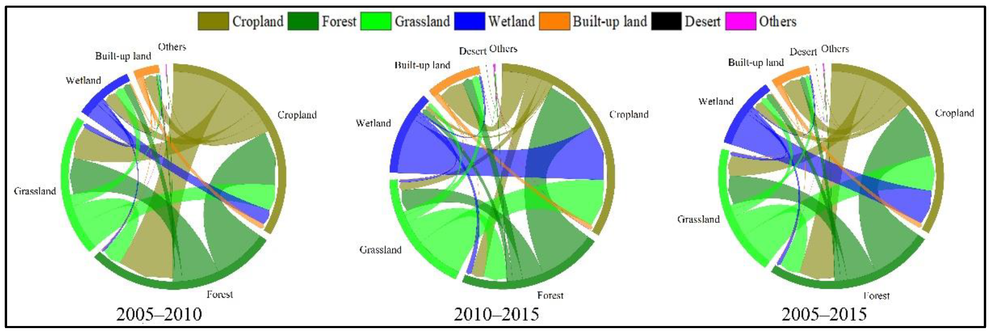
3.1. Evolution of Ecosystem Pattern

From 2005 to 2015, the classification result of ecosystem patterns in the NFB is shown in Figure 3 and

Table 4. Statistics of different land use types of ecosystem patterns of the NFB from 2005–2015.

Ecosystem Pattern	2005		2010		2015
	Area (km2)	Percent (%)	Area (km2)	Percent (%)	Area (km2)	Percent (%)
Forest	110,260	17.92	110,164	17.90	110,838	18.01
Grassland	391,951	63.68	391,810	63.66	391,497	63.61
Wetland	80,262	13.04	80,377	13.06	80,080	13.01
Cropland	26,738	4.34	26,799	4.35	26,492	4.30
Built-up land	5607	0.91	5665	0.92	5900	0.96
Desert	172	0.03	172	0.03	173	0.03
Others	468	0.08	471	0.08	478	0.08
Total amount	615,458	100	615,458	100	615,458	100

. It can be seen that forest, grassland, and cropland were the main ecosystems. Statistics showed that the area of these three ecosystems was about 580,000 km², accounting for more than 94%. Wetland, built-up land, desert, and other ecosystems were scattered in the NFB. During 2005–2015, the structure of ecosystems in the NFB was relatively stable, but conversions between different types were frequent due to climate change, human activities, and other interference factors. Ecosystem transfer in the NFB during 2005–2015 is shown in Figure 4.

From 2005 to 2010, the areas of cropland and forest decreased, and the areas of grassland, wetland, and built-up land increased. Cropland was mainly converted into forest, about 378 km², followed by grassland, about 219 km². However, some grassland and forest were still transformed into cropland, with a conversion area of about 537 km². This showed that the project of returning cropland to forest and grassland in the important ecological function areas of the NFB had achieved good results. However, there were still some cases of deforestation and increasing human disturbance.

From 2010 to 2015, large areas of grassland, forest, and wetland were transformed into cropland and built-up land. During this period, cropland conversion was the main driver of the increase in built-up land areas, with about 153 km² of cropland converted into built-up land. However, there were still 951 km² of grassland, forest, and wetland transformed into cropland. During 2010–2015, the area of cropland and built-up land increased steadily, and the interference of social factors such as human activities was significantly higher than that between 2005–2010.

Between 2005 and 2015, there were more mutual transformations between cropland and forest, forest and grassland, cropland and grassland, built-up land and cropland, cropland and wetland. Among them, the forest type was transferred out of 1214 km², mainly to cropland and grassland. The area transferred to other land was relatively small, indicating that the protection of forests had a certain effect in 10 years. A total of 854 km² area of grassland changed, mainly converted to forest and cropland. The outflow of cropland mainly flowed to forest, grassland, built-up land, and wetland, with areas of 449 km², 260 km², 230 km^2, and 112 km², respectively. The built-up land area increased yearly, and the conversion speed was gradually accelerating. The increasing area mainly came from cropland, forest, and grassland. The wetland area mainly flowed to cropland, and other landscape types had almost no change. Overall, the project of returning cropland to forest and grassland had achieved a good result. Still, the areas of cropland and the built-up land areas had gradually increased in the past 10 years, indicating that the impact of human interference, such as the blind expansion of cultivated land and construction land on the NFB, was gradually increasing, which required us to pay more attention to and the protection of its ecosystem needed to be continued.

Forward/reverse conversion rates (TFR and RFR) of ecosystems in the NFB for 2005–2010 and 2010–2015 are shown in

Table 5. Forward/reverse conversion rate in the NFB.

Year.	Transformation Direction	Cropland	Forest	Grassland	Wetland	Built-Up Land	Desert	Others
2005–2010	TFR	0.124	0.003	0.049	0.000	0.178	0.000	0.043
	RFR	0.015	0.032	0.046	0.113	0.000	0.000	0.000
2010–2015	TFR	0.027	0.002	0.039	0.000	0.124	0.000	0.085
	RFR	0.029	0.027	0.082	0.288	0.000	0.000	0.000

Note: TFR is the forward transformation rate, 100%; and RTR is the reverse transformation rate, 100%.

. During these two periods, the RFR of the forest and wetland was greater than TFR, indicating that these two ecosystem types were more transformed to lower ecosystem types. The TFR of built-up land and other ecosystem types was higher than that of RFR, indicating that ecological control projects had also achieved good results and progress in the NFB. During the two periods, RFRs of the forest, grassland, and wetland were high and showed an upward trend between 2010 and 2015, indicating that there were still some problems to be solved in the NFB. At the same time, among all ecosystems, the TFR of built-up land, cropland, and other ecosystem types was significantly higher than that of the other four ecosystems, indicating that the implementation of policies such as returning cropland to forest and grassland and limiting the scope and extent of economic activities had a great impact on the protection and improvement of ecosystems.

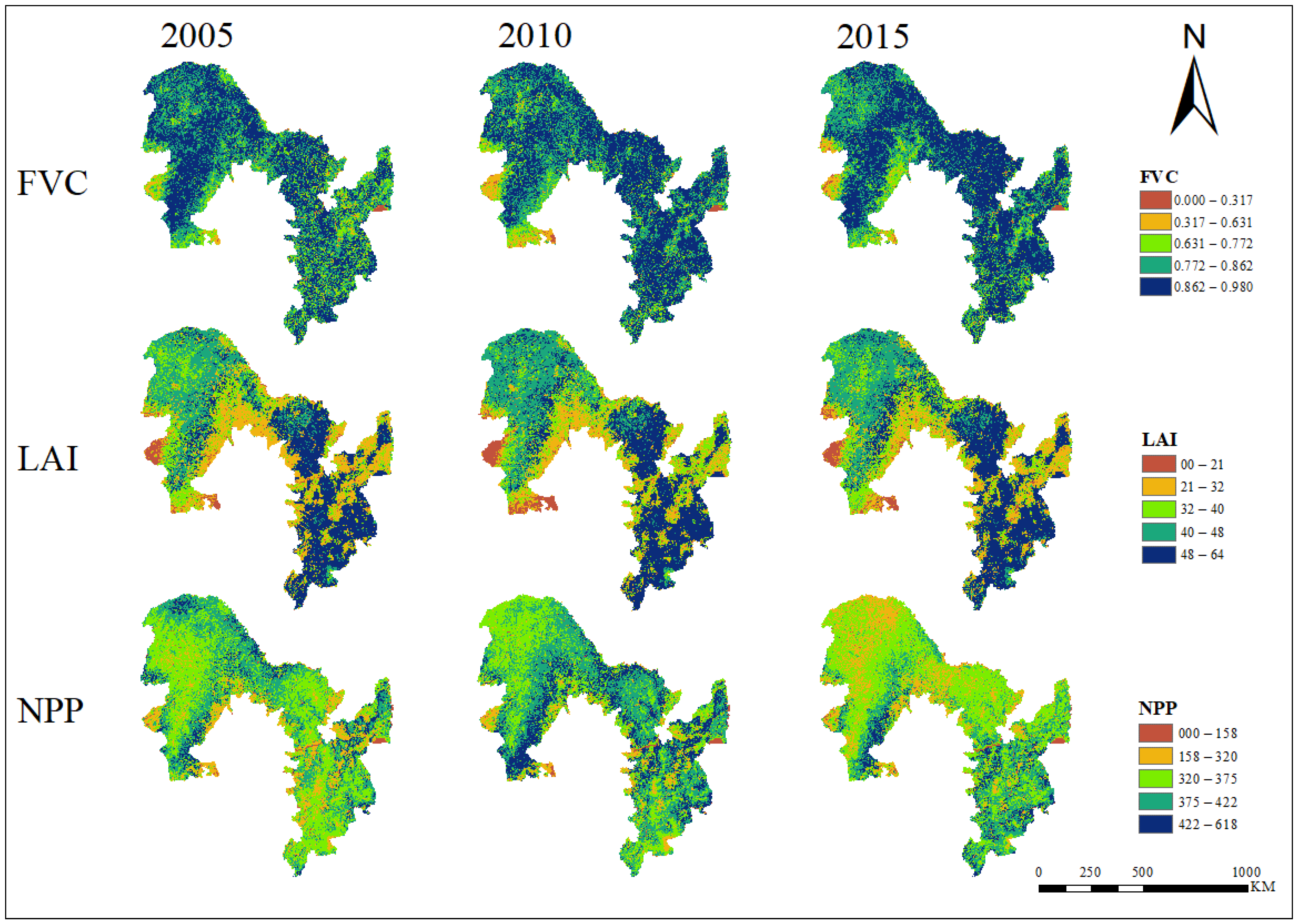
3.2. Spatial Patterns and Variation of EQ

The results of NPP, LAI, and FVC were divided into five grades (excellent, good, middle, general, and poor) according to the natural breakpoint method. The spatial distribution map of EQ and the area transfer matrix of each EQ grade were obtained by spatial statistical analysis, and the quantitative spatial and temporal analysis of EQ was carried out. The spatial distribution of NPP, LAI, and FVC at different levels in the NFB from 2005 to 2015 is shown in Figure 5.

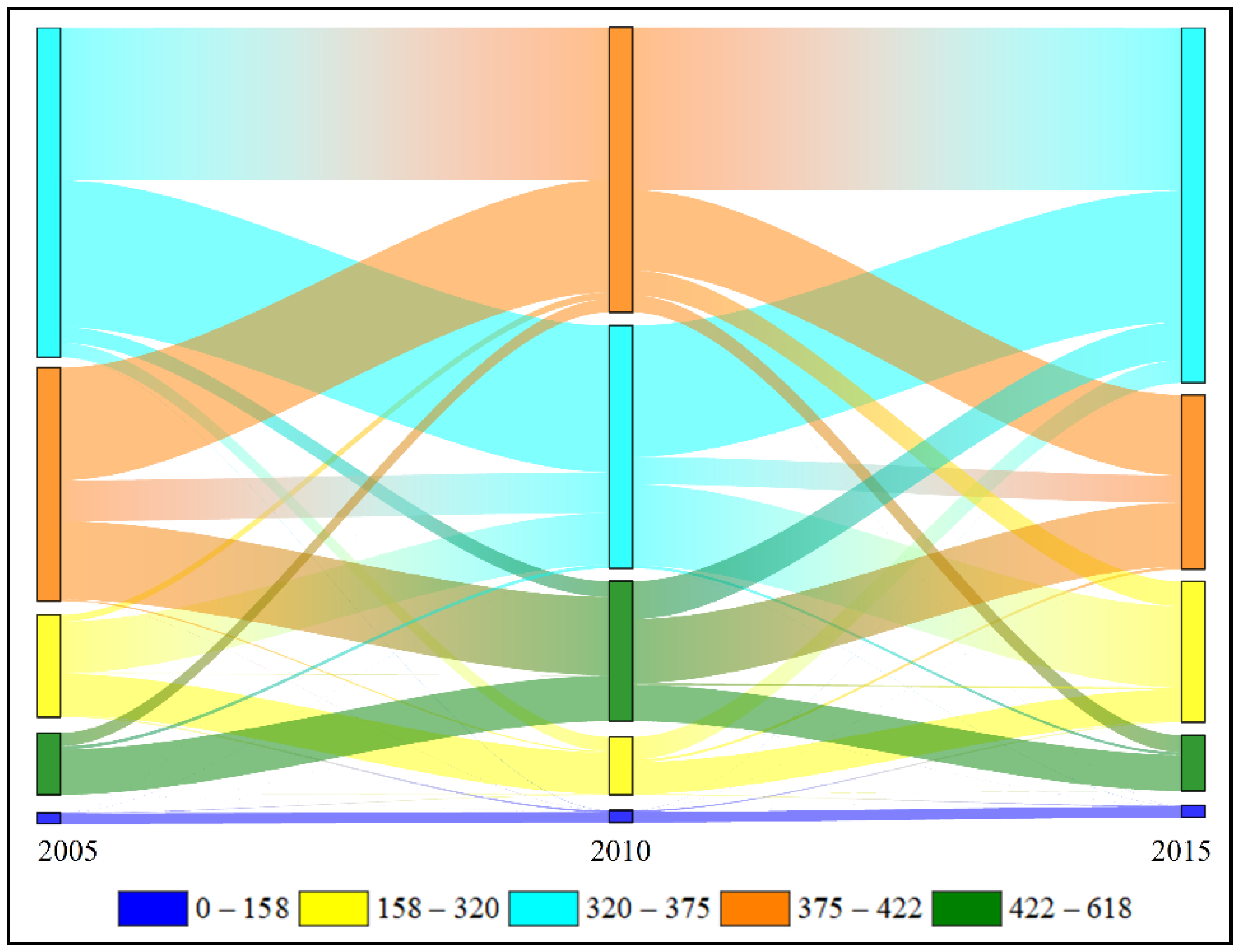
3.2.1. Dynamic Characteristics of NPP

It can be seen from Figure 5 that in 2005, the areas with high NPP were mainly distributed in the south of GKM, the north of GKM, the north of LKM, and the east of CBM, while other areas were mainly dominated by middle NPP. In addition to the decline in northern GKM in 2010, other regions had increased significantly; however, by 2015, the GKM, the LKM, and the northeast of CBM showed a sharp downward trend, and only the central part of CBM remained stable, and the southern part improved. Figure 6 and

Table 6. Area transfer matrix of different NPP levels in the NFB from 2005–2015.

Year	NPP Level	Poor (km2)	Fair (km2)	Middle (km2)	Good (km2)	Excellent (km2)
2005–2010	Poor		592	45	14	4
	Fair	1338		43,274	5649	334
	Middle	199	11,871		127,125	13,196
	Good	79	1157	34,089		65,354
	Excellent	11	199	2762	10,975
2010–2015	Poor		1130	96	34	3
	Fair	745		18,869	2133	123
	Middle	112	67,789		22,850	2184
	Good	39	20,709	135,889		14,126
	Excellent	33	1393	31,646	53,501
2005–2015	Poor		766	80	25	3
	Fair	1111		38,243	6113	764
	Middle	236	53,261		57,227	8878
	Good	127	22,224	89,167		21,390
	Excellent	38	2355	13,456	20,382

showed that NPP in the NFB was mainly middle-quality and good-quality areas. During 2005–2010, the area of general and middle grades showed a significant downward trend, while that of poor, good, and excellent grades showed an increasing trend. The area ratio of good and excellent NPP increased rapidly. The largest transformation area was the middle grade, mainly to good grade, and the transfer area was 127,125 km². In general, the period showed a trend of transformation in a good direction. During 2010–2015, the overall trend was opposite to that before, and the areas of poor, good, and high-quality grades mainly showed a downward trend, while those of middle and general grades showed an increasing trend. The largest transformation area was the good grade, mainly middle grade, and the transfer area was 135,889 km². The overall period showed a certain degree of quality decline. This indicated that the NPP in the NFB increased from 2005 to 2010, and it may decrease from 2010 to 2015 due to ecological damage and environmental degradation.

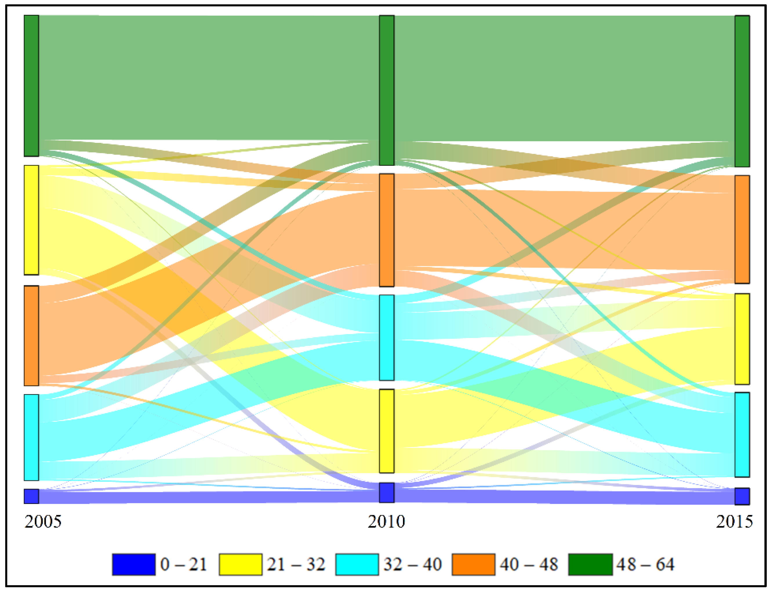
3.2.2. Dynamic Characteristics of LAI

It can be seen from Figure 5 that the distribution of high LAI areas was similar to that of FVC, which was mainly distributed in the middle of the three mountains in the NFB, and the edge areas of northeast CBM, southwest LKM and southern GKM were relatively low. In 2015, the area with an LAI of greater than 48 was mainly distributed in the central part of LKM and the central and southern part of CBM, with an area of 206,334.50 km², accounting for 33.50%. The area with an LAI of less than 32 was mainly located northeast of CBM and on the edge of the southern GKM, with an area of 146,782.5 km², accounting for 23.82%.

It can be seen from Figure 7 and

Table 7. Area transfer matrix of different LAI levels in the NFB from 2005–2015.

Year	LAI Level	Poor (km2)	Fair (km2)	Middle (km2)	Good (km2)	Excellent (km2)
2005–2010	Poor		3037.25	534.50	72.00	383.25
	Fair	9115.00		44,022.50	10,289.75	3443.00
	Middle	2052.00	23,814.50		30,719.25	7123.00
	Good	159.00	3325.25	10,524.75		23,651.75
	Excellent	113.50	1179.75	7669.50	13,580.00
2010–2015	Poor		6478.25	2084.50	381.00	387.75
	Fair	3873.50		30,428.50	5348.50	2170.00
	Middle	644.50	37,092.00		12,495.75	11,521.75
	Good	77.50	5725.00	22,008.25		20,833.25
	Excellent	338.25	2606.00	6227.00	23,994.50
2005–2015	Poor		3700.25	877.75	193.50	465.75
	Fair	6822.00		39,639.50	11,397.50	4577.00
	Middle	1096.50	27,113.00		23,052.25	11,783.50
	Good	226.50	4274.25	13,668.00		21,271.25
	Excellent	107.00	1915.75	6896.75	15,372.75

that in addition to the small area of poor quality, the other four grades were almost similar, and the area of excellent grade had always been the highest. During 2005–2010, areas at the general and middle levels showed a decreasing trend, while areas at the poor, good and excellent levels showed an increasing trend. The largest transformation area was from fair grade to middle grade, and the transfer area was 44,022.50 km². The period generally showed a trend of transformation in a good direction. During 2010–2015, the area of some middle and general grades increased and decreased, but the area of excellent and good grades continued to increase. The largest transformation area was from middle to fair grade, and the transfer area was 127,125 km². The overall trend was relatively stable. It showed that the LAI of the NFB had been continuously improved and enhanced during 2005–2015, and the policy of returning cropland to forest and grassland had protected and improved its ecosystem.

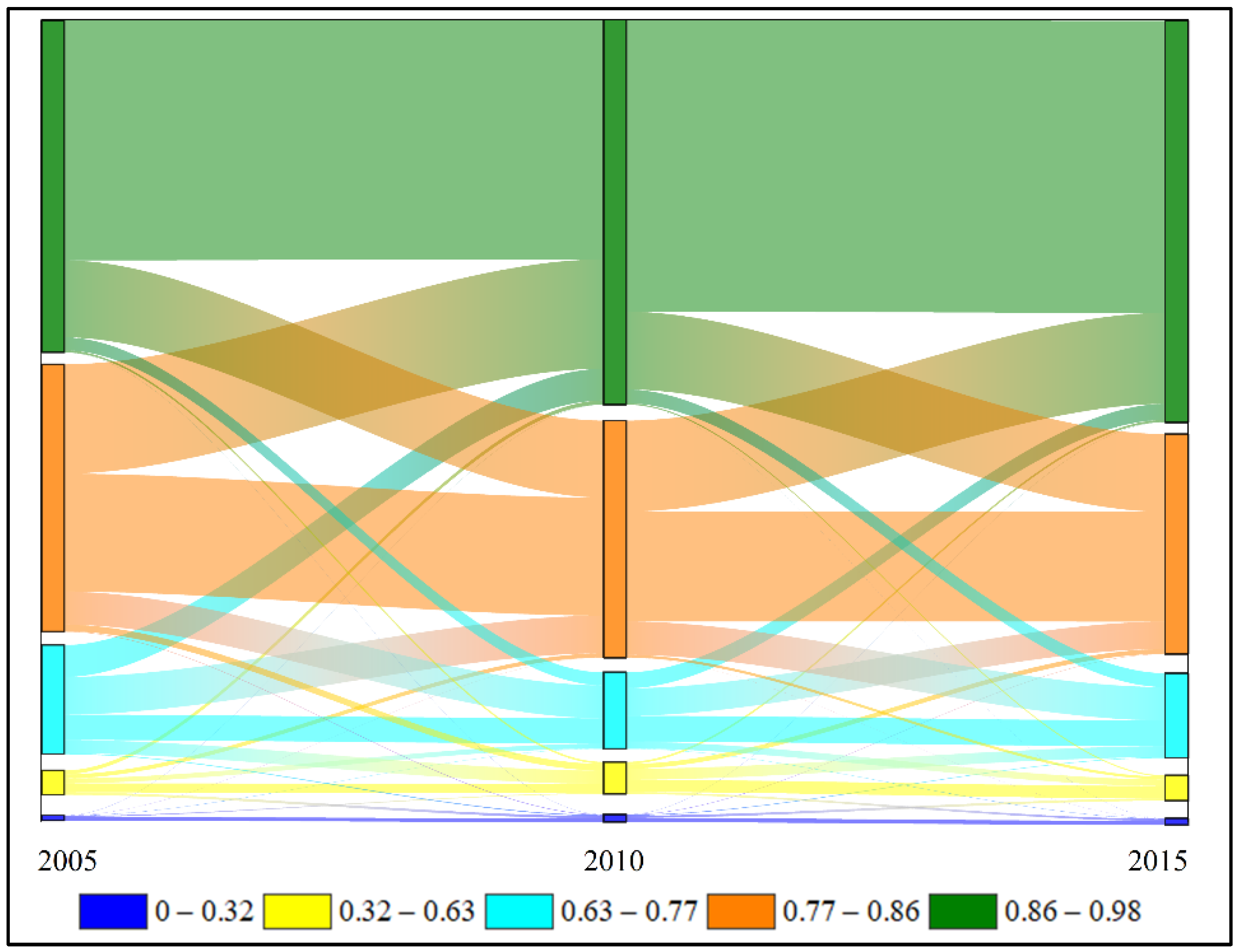
3.2.3. Dynamic Characteristics of FVC

It can be seen from Figure 5 that the high-level regions were mainly distributed in most parts of the NFB, and most of them were concentrated in the middle of the three mountains of the NFB. The areas with low FVC were mainly distributed in the edge area of the southern GKM and the northeast of CBM. The cropland area in this area was large, and the FVC value was low. During 2005–2015, except for the southern edge of the GKM, FVC decreased, and the other regions showed an upward trend.

It can be seen from Figure 8 and

Table 8. Area transfer matrix of different FVC levels in the NFB from 2005–2015.

Year	FVC Level	Poor (km2)	Fair (km2)	Middle (km2)	Good (km2)	Excellent (km2)
2005–2010	Poor		811.75	230.75	126.75	157.25
	Fair	2063.50		4124.00	3458.75	3274.50
	Middle	761.50	11,163.50		31,493.50	26,591.25
	Good	438.25	5585.00	27,511.75		91,299.25
	Excellent	126.00	1643.50	10,801.25	64,285.25
2010–2015	Poor		1970.75	545.00	318.50	149.25
	Fair	1698.75		9140.25	3963.25	1783.00
	Middle	273.75	5699.75		22,891.00	13,337.00
	Good	73.75	2252.25	27,844.25		76,032.50
	Excellent	47.00	1069.25	11,636.00	64,940.00
2005–2015	Poor		937.00	256.75	152.50	178.25
	Fair	1929.00		4743.50	3284.75	3353.25
	Middle	534.00	8397.75		29,159.75	27,175.25
	Good	184.75	3720.50	31,297.00		93,027.75
	Excellent	49.25	945.00	8591.50	56,073.00

that the area with good and excellent grades quality FVC accounted for a large proportion, accounting for about 81% of the total area. During 2005–2010, the area of excellence level had increased significantly, and its proportion exceeded half of the total area. The poor grade mainly turned to the general grade; the general grade was mainly transferred to the middle grade; the middle grade mainly turned to the good grade; the good grade mainly turned to the excellent grade, and the excellent grade mainly turned to a good grade. During 2010–2015, the area at the excellent and middle levels continued to increase, while the area at the poor and general levels decreased; the poor grade mainly turned to the general grade, the general grade primarily turned to the middle grade, the middle grade mainly turned to the good grade, the good grade mainly turned to the excellent grade, the excellent grade mainly turned to good grade. During 2005–2015, it generally showed a trend of good transformation, indicating that FVC in the NFB had been in a better situation during this period and had continued to improve and enhance.

3.3. Spatial Patterns and Variation of ES

3.3.1. Habitat Provision Service

The high value of HP was mainly distributed in the middle of GKM, LKM, and CBM, while the low value was mainly distributed around them (Figure 9). Overall, HP in forest areas was higher than other spatial pattern types such as cropland and built-up land and showed a decreasing trend from inside to outside. From the point of view of the time change, it was mainly to maintain a relatively stable state, the overall change was small, from 2005 to 2015 showed a slight upward trend, and 2010–2015 compared to 2005–2010 upward trend was more obvious. During 2005–2010, the overall decreasing and increasing areas accounted for about 37.60 % and 45.05%, respectively. The decreasing areas were mainly located where cropland and built-up land were located, while the increasing areas were mainly located where LKM and CBM forests were distributed. From 2010 to 2015, the areas where HP increased and decreased accounted for about 22.54% and 55.02%, respectively. The increased areas were mainly located in the eastern and southern parts of the GKM and the areas where cropland was distributed. The main reason may be that forest protection measures such as returning cropland to forest and grassland were implemented there, while the reduced areas were mainly distributed in some areas of the western GKM.

3.3.2. Soil Conservation Service

The SCS of the NFB was generally low. The high value of SCS was mainly distributed in the south of CBM, and the middle of the three mountains was also mainly about the middle value. Most areas of SCS were low value (Figure 9). It remained stable over time, with very small overall changes, with a slight upward trend in 2005–2010 and a slight downward trend in 2010–2015.

3.3.3. Carbon Sequestration Service

The spatial distribution of C in the southeast was higher than that in the northwest (Figure 9). The highest value appeared in the south of CBM, and the lowest value appeared in the southwest of GKM. For the time change, the whole area of GKM had a low value in 2005, and then the value in the eastern and northern regions improved. From 2005 to 2010, the increased area of C (71.68%) was significantly larger than the decreased area (27.42%), showing an upward trend. The increase of C was mainly concentrated in the northern GKM and the whole area of LKM and CBM, and only the southwestern GKM showed a significant downward trend. The southwestern GKM had more cropland area, so this sharp decline may be related to increased disturbance of human activities during the period. From 2010 to 2015, the decrease in the C area (54.75%) was greater than the increase (44.36%), showing a downward trend in general. The C value in the southwest GKM increased, and the decrease was mainly distributed in the northern GKM and the southern CBM.

3.3.4. Sand-Stabilization Service

The high SSS value was mainly distributed in the northeast of CBM and the southwest of GKM, while the low SSS value was mainly distributed in the north of GKM, the middle of LKM, and the south of CBM (Figure 9). During 2005–2010, SSS showed a downward trend, but from 2010–2015 showed an upward trend. From 2005 to 2010, the proportion of SSS increased (11.03%) and decreased (15.99%) relatively small, most of which remained stable (72.98%). From 2010 to 2015, the increased area (19.36%) was improved compared with the previous, but most areas remained relatively stable (73.02%). During the two periods, the increased or decreased areas were mainly distributed in the areas where other spatial pattern types except forests were located, while the areas where forests were located remained relatively stable.

3.3.5. Water Conservation Service

The high value of WCS was mainly distributed in the southern region of the CBM. The middle of the three mountains of the GKM, the LKM, and the CBM also maintained a middle value, while the low value was mainly distributed in the northeast of the CBM, the southwest of the LKM, and the southern edge of the GKM. The WCS of the whole area of the GKM was lower (Figure 9). From the perspective of the time change, from 2005 to 2010, WCS showed a significant upward trend, and 59.75% of the regions increased. The regions with obvious increase were the central GKM, the central LKM, and the southern CBM. From 2010 to 2015, the WCS showed a significant downward trend, and the decreased area (54.13%) was greater than the increased area (23.90%). The decreased area was mainly distributed in the central part of the GKMs and the southern part of the CBM, especially on the southern edge of the CBM.

3.4. Comprehensive Ecosystem Index Evaluation

Firstly, the weight coefficients of the relevant indicators of the ecosystem in the NFB were determined by the AHP, which passed the consistency test, and the weight setting was reasonable. Then, ArcGIS was used to obtain the spatial distribution map of the comprehensive evaluation index of the ecosystem in different years. Finally, it was divided into five grades according to the natural breakpoint method and manual adjustment, and the data were statistically analyzed (as shown in Figure 10 and

Table 9. Statistics of different levels of comprehensive index data of the NFB from 2005–2015.

Comprehensive Index Level	2005		2010		2015
	Area (km2)	Percent (%)	Area (km2)	Percent (%)	Area (km2)	Percent (%)
Poor (0.013–0.262)	33,456	5.21	45,326	7.06	27,521	4.29
Fair (0.262–0.333)	131,000	20.40	132,402	20.62	118,302	18.42
Middle (0.333–0.399)	177,052	27.57	174,635	27.19	147,437	22.96
Good (0.399–0.471)	229,065	35.67	223,391	34.78	230,204	35.85
Excellent (0.471–0.746)	71,641	11.16	66,460	10.35	118,750	18.49
Total amount	642,214	100	642,214	100	642,214	100

).

The spatial and temporal distributions of the ecosystem comprehensive evaluation index in the NFB in 2005, 2010, and 2015 are shown in Figure 10. The areas with a high spatial distribution value of the ecosystem in the NFB were mainly distributed in the southern part of CBM, the central part of LKM, and the northwestern part of GKM, while the northeastern part of CBM, the southwestern part of LKM and the marginal area of southern GKM were relatively low. During 2005–2010, the value of the southern edge of GKM showed a significant decline, and the eastern and central CBM and the central LKM also showed a slight decline. During 2010–2015, the change in the ecosystem comprehensive evaluation index showed an almost opposite trend; that is, the values of southern GKM and central LKM increased significantly, and other regions also increased to varying degrees. During the whole study period from 2005 to 2015, except for the decrease in the value around the marginal area in the southern GKM, the value in other regions showed an upward trend, which was closely related to a series of protection and improvement measures such as the “two ecological barriers and three shelters” national ecological stability pattern strategy, grain for green project, and comprehensive management of soil and water loss carried out in the NFB.

According to the change level of the ecosystem comprehensive evaluation index (0.013–0.746, Table 9), the change of the ecosystem comprehensive evaluation index was divided into five grades: excellent, good, middle, general, and poor. The area of the five grades of the ecosystem comprehensive evaluation index in 2005, 2010, and 2015 is shown in Table 4. Specifically, in 2005, the area with good and middle grades accounted for a large proportion (total 63.24%), and the proportion of poor grade was very small (5.21%). This indicated that the overall quality of ecosystems in 2005 was good. The grade area ratio in 2010 was consistent with 2005, and the overall area changed little. However, on the whole, some areas fell from the middle, good and excellent grades to the poor and general grades, indicating that during this period, the NFB faced some problems such as ecological destruction and environmental degradation. In 2015, the good grade area was the largest (230,204 km²), and the poor and middle-grade areas significantly decreased. Good and excellent areas had been significantly increased, mainly from poor, general, and middle regions, indicating the effectiveness of the “two ecological barriers and three shelters” national ecological stability pattern strategy implemented in the NFB.

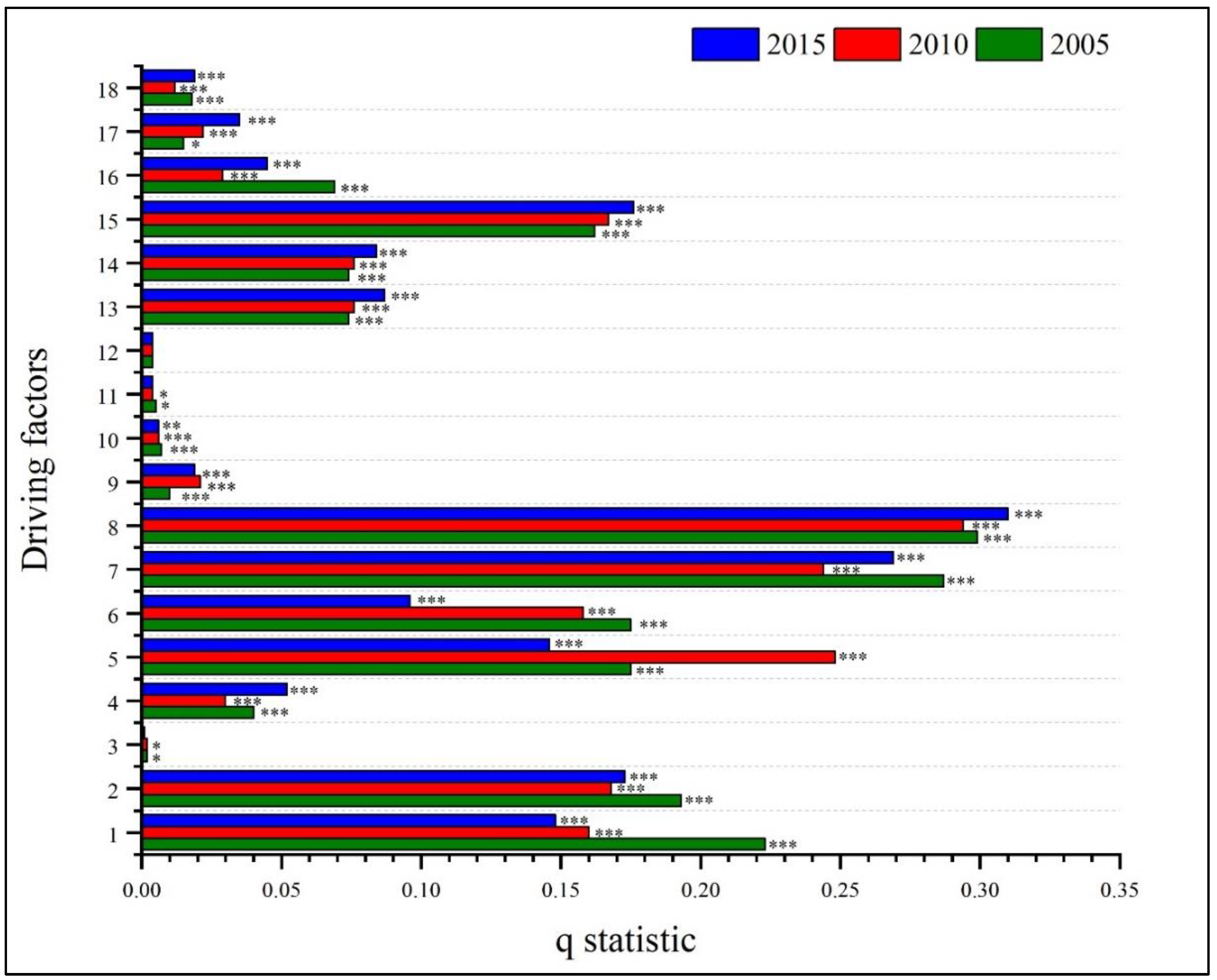
3.5. Driving Force Analysis

In this study, a 10 km × 10 km grid was used to generate 7119 points in the study area in ArcGIS. After analysis, the influence value and driving effect of each index factor on the ecosystem evolution in the NFB were obtained (as shown in Figure 11).

It can be seen from Figure 11 that land use/cover, climate (annual average rainfall, etc.), and human disturbance (GDP, etc.) were related potential factors affecting the ecosystem evolution of the NFB. Most of the driving factors in the three periods of 2005, 2010, and 2015 were sufficient for the evolution of the NFB ecosystem (p < 0.05), indicating that the evaluation system constructed in this study was reasonable. In 2005, the three most influential factors in the evolution of the NFB ecosystem were forest, cropland, and elevation, and their influence values were 0.299, 0.287, and 0.223, respectively. The influence of driving factors from high to low were terrain factors, soil factors, meteorological factors, and human social factors. The influence of some driving factors in 2010 and 2015 differed from 2005, but the impact of the overall driving factors showed little change. Land use types had the greatest influence on ecosystem evolution in the NFB, and cropland and forest had a more significant influence than wetland, grassland, built-up land, and other types. The influence value of NPP remained at a middle-to-high level during the study period, and its influence value was more obvious than other factors. Regarding topographic factors, the influence value of elevation and slope was relatively significant, while the influence of slope direction was not big. In terms of soil factors, the influence of sand was larger than the other three factors. The influence of temperature on climate factors had been small, while the influence of precipitation is more obvious; even in 2010, it was only lower than that of the forest. In terms of social factors, the influences of human activity factors such as GDP and population density were small. Still, their visibility was extremely significant (p < 0.001, except for the GDP factor in 2005), indicating that human disturbance factors such as GDP and population density were also potential factors affecting the evolution of the NFB ecosystem.

4. Discussion

4.1. Advantages of the Integrated Ecosystem Assessment Index

In this study, the AHP was used to obtain the comprehensive evaluation index of the ecosystem, and a variety of methods were used to evaluate the ecosystem of the NFB comprehensively. The results showed that the landscape types of the NFB were mainly forest, cropland, and grassland, and the study showed a stable state as a whole. However, the areas of cropland and built-up land were still expanding, which needed more attention. This result was consistent with the research of others [3]. Compared with the principal component analysis method [56,57,58,59,60] that has been studied more before, the results showed that the ecosystem comprehensive evaluation index created by AHP in this study can also carry out a comprehensive ecosystem assessment. The results showed that the areas with a good ecosystem environment in the NFB were mainly distributed in the south of CBM, the middle of LKM, and the northwest of GKM and had a significant improvement and improvement trend with time. In contrast, the areas around the southeast and southwest of GKM were relatively poor, similar to some previous research results [2,12]. The reason may be that the good region was mainly located in the main part of the three mountains and was dominated by forests, with lush vegetation and less human disturbance, so the comprehensive index was high. The poor area may be due to the northeast plain, arable land to the NFB continued to expand, and more serious interference from human activities, resulting in the poor composite index. Throughout 2005–2015, the ecosystem in the NFB was in a relatively good state as a whole, and maintained a trend of improvement, which was closely related to a series of protection and improvement measures such as the “two ecological barriers and three shelters” national ecological stability pattern strategy [61], the project of returning cropland to forest and grassland [62,63,64], and the comprehensive control of soil and water loss. By comparing the results of landscape pattern, ES, and EQ in the NFB in this study, it could be seen that the evaluation results based on a single factor were uncertain and limited. And there were conflicts and contradictions between the evaluation results of different factors. Thus the ecosystem cannot be accurately evaluated. Based on these shortcomings and deficiencies, some researchers chose the method of constructing RSEI to analyze the ecosystem evolution [23,65,66] to obtain more accurate and comprehensive results. However, the construction of the remote sensing ecological index will ignore the impact of the land use/cover change process on the structure and function of the ecosystem. Therefore, in this study, combined with multiple indicators such as land use/cover, ES, and EQ, it was more accurate, systematic and comprehensive to evaluate the evolution of the NFB ecosystem by constructing the ecosystem comprehensive evaluation index.

4.2. Uncertainty of Driving Force Analysis

The driving force analysis showed that the natural factors had a great influence on the ecosystem of the NFB. Among them, land use type was an important factor affecting the ecosystem evolution of the NFB, which was consistent with the research results of Su and Zhu et al. [3,12]. However, the influence value of NPP in the study of Zhu et al. was more significant than in this study, which may be related to the difference in data sources and the number of grid points. The influence of elevation and slope was larger, probably because the higher and steep areas were covered by vegetation or less affected by human activities; the ranking of precipitation had been ahead, and its influence value rose to second in 2010, which was consistent with some studies [67,68,69]. Precipitation was one of the main factors affecting vegetation growth, so it also affected the evolution of ecosystems. The impact of human activity factors such as population density and GDP on the evolution of the ecosystem in the NFB was small, consistent with the results of Zhu et al. [12]. This may be because the overall social and economic activities in the NFB were less, and the population density and GDP were relatively sparse. In addition, this study only selected population density, GDP, and road as the three human activity factors for analysis. It did not comprehensively and specifically analyze what human social factors will affect the evolution of the NFB ecosystem, resulting in uncertainty in the final analysis of the results. Currently, there is no consistent method to evaluate the driving force that affects the evolution of the ecosystem. The methods for analyzing the driving force of the ecosystem mainly included correlation analysis, residual or redundancy analysis, and different methods may produce different results. Zhu et al. [12] found that the influence of social factors such as GDP and population density on the ecosystem of the NFB was not obvious; Sun et al. [3] indicated that human disturbance factors such as urban expansion were the main reason for the decrease of carbon sequestration in the NFB. As for the drought index, Wang et al. [70] considered that it was the main factor driving the growth of forest vegetation and the change of carbon sink function in Northeast China. The results of driving force analysis in this study were similar to those in Zhu et al. [12], although there were still differences in some factors and effects. The selection of driving force indicators and methods may have an important impact on the final results and the subsequent management of the ecosystem. Therefore, the accurate analysis of driving force still needs further continuous research.

4.3. Limitations of Current Research

This study still had some deficiencies and needed to be further studied. Although the landscape pattern of the NFB ecosystem analyzed in this study could roughly reflect the changes during the entire study period. It cannot accurately reflect the evolution of the NFB ecosystem pattern and the relationship between horizontal and vertical pattern structure and quality function. This still needs more detailed research. And the remote sensing data used in this study, due to sources and other limitations, only selected 2005, 2010, and 2015 data, and remote sensing data resolution was relatively low, which may affect the accuracy of the results. In addition, this study only conducted quantitative spatio-temporal assessments of ES and EQ in the NFB. In the future, the collaboration and trade-off between ES and quality will be explored. In addition, in the driving force analysis, due to the limitation of data sources, only three human activity factors, namely GDP, population density, and road, were selected for analysis. However, these three factors were relatively macroscopic, which cannot reflect the specific human disturbance activities that affect the evolution of the ecosystem in the NFB, which was not conducive to the application in a specific practice. In future research, more comprehensive driving factors can be added to analyze, and the evaluation system framework can be further optimized to more comprehensively and accurately evaluate the changes in the ecosystem environment and the impact of driving factors.

5. Conclusions

In this study, the multi-source remote sensing data and multiple indicators were used to construct the comprehensive evaluation ecosystem index of the NFB. The changes and driving forces of the NFB ecosystem from 2005 to 2015 were evaluated based on the PNTIL model, transfer matrix, geographical detector, and other methods. Using an ecosystem comprehensive evaluation index can avoid the shortcomings of uncertainty and limitation based on single factor evaluation results to evaluate the evolution of the NFB ecosystem more systematically, comprehensively, and accurately. The main conclusions are as follows:

The landscape pattern types of the NFB were mainly forest, cropland, and grassland, and the overall landscape pattern of the NFB was stable during 2005–2015. The comprehensive assessment of the ecosystem index showed that the areas with a good ecosystem environment in the NFB were mainly distributed in the southern CBM, the central LKM, and the northwestern GKM, while the northeastern CBM, the southwestern LKM, and the marginal areas of southern GKM were relatively poor. During 2005–2015, the overall ecosystem of the NFB was in a relatively good state and maintained a trend of improvement in a good direction. However, during 2005–2010, there were still some anthropogenic disturbances that led to a decline in the comprehensive index of some regions. The driving force analysis showed that natural factors had a great influence on the ecosystem of the NFB. Land use/cover was an important driving factor affecting the ecosystem evolution of the NFB. Climate (annual average rainfall, etc.) and human disturbance (GDP, etc.) were potential factors affecting the ecosystem evolution of the NFB. The results showed that in the past 10 years, the EQ of the NFB was generally in a good state and continued to improve, but the expansion of cropland and built-up land in some areas continued to increase, which needed to be paid more attention.

In the future, relevant research will continue to analyze the synergy and trade-off relationship of various ES and their spatial differentiation and further regionalize ES to explore the formation mechanism of the synergy and trade-off relationship of different ES. The correlation between synergy and trade-off relationship with the main driving forces obtained in the driving force analysis of this study can also be further studied. At the same time, the optimization of the evaluation system framework and the reasonable and comprehensive selection of impact factors still need to be further improved, including the prospect of the change characteristics of the ecosystem comprehensive index with the above factors. It is hoped that a series of studies will provide a more scientific and comprehensive reference for the ecosystem stability and improvement of the NFB.

References

1. Sun, B. Decade Change of Ecosystem Pattern, Quality, Service Function and Stress in the Northeastern Forest Regions (2000–2010); University of Chinese Academy of Sciences: Beijing, China, 2015. [Google Scholar]
2. Sun, B.; Zhao, H.; Lu, F.; Wang, X. Spatial and temporal patterns of carbon sequestration in the Northeastern Forest Regions and its impact factors analysis. Acta Ecol. Sin. 2018, 38, 4975–4983. [Google Scholar]
3. Su, K.; Wang, Y.; Sun, X.; Yue, D. Landscape pattern change and prediction of Northeast Forest Belt based on GIS and RS. Trans. Chin. Soc. Agric. Mach. 2019, 50, 195–204. [Google Scholar]
4. Kong, L.; Zhang, L.; Zheng, H.; Xu, W.; Xiao, Y.; Ouyang, Z. Driving forces behind ecosystem spatial changes in the Yangtze River Basin. Acta Ecol. Sin. 2018, 38, 741–749. [Google Scholar]
5. Borzì, L.; Anfuso, G.; Manno, G.; Distefano, S.; Urso, S.; Chiarella, D.; Di Stefano, A. Shoreline evolution and environmental changes at the NW Area of the Gulf of Gela (Sicily, Italy). Land 2021, 10, 1034. [Google Scholar] [CrossRef]
6. Aho, K.; Weaver, T. Alpine nodal ecology and ecosystem evolution in the North-Central Rockies (Mount Washburn; Yellowstone National Park, Wyoming). Arct. Antarct. Alp. Res. 2010, 42, 139–151. [Google Scholar] [CrossRef]
7. Huang, J.; Sun, L.; Wang, X.; Wang, Y.; Huang, T. Ecosystem evolution of seal colony and the influencing factors in the 20th century on Fildes Peninsula, West Antarctica. J. Environ. Sci. 2011, 23, 1431–1436. [Google Scholar] [CrossRef]
8. Li, C.; Zhao, J.; Zhuang, Z.; Gu, S. Spatiotemporal dynamics and influencing factors of ecosystem service trade-offs in the Yangtze River Delta urban agglomeration. Acta Ecol. Sin. 2022, 14, 1–13. [Google Scholar]
9. Apostolopoulos, D.N.; Avramidis, P.; Nikolakopoulos, K.G. Estimating quantitative morphometric parameters and spatiotemporal evolution of the Prokopos Lagoon using remote sensing techniques. J. Mar. Sci. Eng. 2022, 10, 931. [Google Scholar] [CrossRef]
10. Weng, H.; Gao, Y.; Su, X.; Yang, X.; Cheng, F.; Ma, R.; Liu, Y.; Zhang, W.; Zheng, L. Spatial-temporal changes and driving force analysis of green space in coastal cities of Southeast China over the past 20 years. Land 2021, 10, 537. [Google Scholar] [CrossRef]
11. Qi, L.; Zhang, Y.; Xu, D.; Zhu, Q.; Zhou, W.; Zhou, L.; Wang, Q.; Yu, D. Trade-offs and synergies of ecosystem services in forest barrier belt of Northeast China. Chin. J. Ecol. 2021, 40, 3401–3411. [Google Scholar] [CrossRef]
12. Zhu, Q.; Wang, Y.; Zhou, W.; Zhou, L.; Yu, D.; Qi, L. Spatiotemporal changes and driving factors of ecological vulnerability in Northeast China forest belt. Chin. J. Ecol. 2021, 40, 3474–3482. [Google Scholar] [CrossRef]
13. Liang, B.; Shi, P.; Wang, W.; Tang, X.; Zhou, W.; Jing, Y. Integrated assessment of ecosystem quality of arid inland river basin based on RS and GIS: A case study on Shiyang River Basin, Northwest China. Chin. J. Appl. Ecol. 2017, 28, 199–209. [Google Scholar] [CrossRef]
14. Zewdie, W.; Csaplovics, E. Identifying categorical land use transition and land degradation in northwestern drylands of Ethiopia. Remote Sens. 2016, 8, 408. [Google Scholar] [CrossRef]
15. Foroumandi, E.; Nourani, V.; Dąbrowska, D.; Kantoush, S.A. Linking spatial-temporal changes of vegetation cover with hydroclimatological variables in terrestrial environments with a focus on the Lake Urmia Basin. Land 2022, 11, 115. [Google Scholar] [CrossRef]
16. Gao, Z.; Bai, Y.; Zhou, L.; Qiao, F.; Song, L.; Chen, X. Characteristics and driving forces of wetland landscape pattern evolution of the city belt along the Yellow River in Ningxia, China. Chin. J. Appl. Ecol. 2020, 31, 3499–3508. [Google Scholar] [CrossRef]
17. Karimi, F.M.; Majid, K.; Mehdi, H.; Jokar, A.J.; Kazem, A.S. A novel method to quantify urban surface ecological poorness zone: A case study of several European cities. Sci. Total Environ. 2021, 757, 143755. [Google Scholar]
18. Mohammad, K.F.; Solmaz, F.; Majid, K.; Asim, B.; Mehdi, H.; Kazem, A.S. Land surface ecological status composition index (LSESCI): A novel remote sensing-based technique for modeling land surface ecological status. Ecol. Indic. 2021, 123, 107375. [Google Scholar]
19. Sajjad, K.S.; Solmaz, A.; Mostafa, G. Spatiotemporal ecological quality assessment of metropolitan cities: A case study of central Iran. Environ. Monit. Assess. 2021, 193, 305. [Google Scholar]
20. Maity, S.; Das, S.; Pattanayak, J.M.; Bera, B.; Shit, K.P. Assessment of ecological environment quality in Kolkata urban agglomeration, India. Urban Ecosyst. 2022, 25, 3. [Google Scholar] [CrossRef]
21. Xu, H. A remote sensing index for assessment of regional ecological changes. China Environ. Sci. 2013, 33, 889–897. [Google Scholar]
22. Xu, H.; Wang, Y.; Guan, H.; Shi, T.; Hu, X. Detecting ecological changes with a remote sensing based ecological Index (RSEI) produced time series and change vector analysis. Remote Sens. 2019, 11, 2345. [Google Scholar] [CrossRef]
23. Yuan, B.; Fu, L.; Zou, Y.; Zhang, S.; Chen, X.; Li, F.; Deng, Z.; Xie, Y. Spatiotemporal change detection of ecological quality and the associated affecting factors in Dongting Lake Basin, based on RSEI. J. Clean. Prod. 2021, 302, 126995. [Google Scholar] [CrossRef]
24. Wang, J. Study on the Spatiotemporal Changes of Ecological Environment and Land Use in the Central Area of Urumqi; Xinjiang University: Urumqi, China, 2021. [Google Scholar]
25. Hu, X.; Xu, H. A new remote sensing index for assessing the spatial heterogeneity in urban ecological quality: A case from Fuzhou City, China. Ecol. Indic. 2018, 89, 11–21. [Google Scholar] [CrossRef]
26. Boori, M.S.; Choudhary, K.; Paringer, R.; Kupriyanov, A. Spatiotemporal ecological vulnerability analysis with statistical correlation based on satellite remote sensing in Samara, Russia. J. Environ. Manag. 2021, 285, 112138. [Google Scholar] [CrossRef]
27. Thiesen, T.; Bhat, M.G.; Liu, H.; Rovira, R. An ecosystem service approach to assessing agro-ecosystems in urban landscapes. Land 2022, 11, 469. [Google Scholar] [CrossRef]
28. Chen, Q.; Chen, Y.; Wang, M.; Jiang, W.; Hou, Y.; Li, Y. Ecosystem quality comprehensive evaluation and change analysis of Dongting Lake in 2001—2010 based on remote sensing. Acta Ecol. Sin. 2015, 35, 4347–4356. [Google Scholar]
29. Chen, H. Establishment and application of wetlands ecosystem services and sustainable ecological evaluation indicators. Water 2017, 9, 197. [Google Scholar] [CrossRef]
30. Yilmaz, F.C.; Zengin, M.; Cure, C.T. Determination of ecologically sensitive areas in Denizli province using geographic information systems (GIS) and analytical hierarchy process (AHP). Environ. Monit. Assess. 2020, 192, 589. [Google Scholar] [CrossRef]
31. Li, W.; Sun, B.; Wang, R.; Cui, L.; Ma, Q.; Zhang, M.; Lei, Y.; Zhu, Y. Various beneficiaries-based analysis on service weight of ecosystem of Momoge Wetland. Water Resour. Hydropower Eng. 2017, 48, 10–15. [Google Scholar] [CrossRef]
32. Morandi, D.T.; França, L.C.d.J.; Menezes, E.S.; Machado, E.L.M.; Silva, M.D.d.; Mucida, D.P. Delimitation of ecological corridors between conservation units in the Brazilian Cerrado using a GIS and AHP approach. Ecol. Indic. 2020, 115, 106440. [Google Scholar] [CrossRef]
33. Zhang, R.; Zhang, X.; Yang, J.; Yuan, H. Wetland ecosystem stability evaluation by using analytical hierarchy process (AHP) approach in Yinchuan Plain, China. Math. Comput. Model. 2013, 57, 366–374. [Google Scholar] [CrossRef]
34. Shafaghat, A.; Ying, O.J.; Keyvanfar, A.; Jamshidnezhad, A.; Ferwati, M.S.; Ahmad, H.; Mohamad, S.; Khorami, M. A treatment wetland park assessment model for evaluating urban ecosystem stability using analytical hierarchy process (AHP). J. Environ. Treat. Tech. 2019, 7, 81–91. [Google Scholar]
35. Guo, Z.; Wei, W.; Pang, S.; Li, Z.; Zhou, J.; Jie, B. Spatio-temporal evolution and motivation analysis of ecological vulnerability in Arid Inland River Basin based on SPCA and remote sensing index: A case study on the Shiyang River Basin. Acta Ecol. Sin. 2019, 39, 2558–2572. [Google Scholar]
36. Chi, W.; Bai, W.; Liu, Z.; Dang, X.; Kuang, W. Wind Erosion in Inner Mongolia Plateau Using the Revised Wind Erosion Equation. Ecol. Environ. Sci. 2018, 27, 1024–1033. [Google Scholar] [CrossRef]
37. Kong, L.; Zheng, H.; Rao, E.; Xiao, Y.; Ouyang, Z.; Li, C. Evaluating indirect and direct effects of eco-restoration policy on soil conservation service in Yangtze River Basin. Sci. Total Environ. 2018, 631–632, 887–894. [Google Scholar] [CrossRef]
38. Fang, Q.; Wang, G.; Zhang, S.; Peng, Y.; Xue, B.; Cao, Y.; Shrestha, S. A novel ecohydrological model by capturing variations in climate change and vegetation coverage in a semi-arid region of China. Environ. Res. 2022, 211, 113085. [Google Scholar] [CrossRef] [PubMed]
39. Deng, Y.; Yao, S.; Hou, M.; Zhang, T.; Lu, Y.; Gong, Z.; Wang, Y. Assessing the effects of the Green for Grain Program on ecosystem carbon storage service by linking the InVEST and FLUS models: A case study of Zichang county in hilly and gully region of Loess Plateau. J. Nat. Resour. 2020, 35, 826–844. [Google Scholar]
40. Nie, Q.; Xu, J.; Ji, M.; Cao, L.; Yang, Y.; Hong, Y. The vegetation coverage dynamic coupling with climatic factors in Northeast China Transect. Environ. Manag. 2012, 50, 405–417. [Google Scholar] [CrossRef]
41. Potter, C.S.; Randerson, J.T.; Field, C.B.; Matson, P.A.; Vitousek, P.M.; Mooney, H.A.; Klooster, S.A. Terrestrial ecosystem production: A process model based on global satellite and surface data. Glob. Biogeochem. Cycles 1993, 7, 811–841. [Google Scholar] [CrossRef]
42. Berdjour, A.; Dugje, I.Y.; Rahman, N.A.; Odoom, D.A.; Kamara, A.Y.; Ajala, S. Direct estimation of maize leaf area index as influenced by organic and inorganic fertilizer rates in Guinea Savanna. J. Agric. Sci. 2020, 12, 66. [Google Scholar] [CrossRef]
43. Zhuo, J.; Zhu, Y.; He, H.; Wang, J.; Dong, J.; Quan, W. Impacts of ecological restoration projects on the ecosystem in the Loess Plateau. Acta Ecol. Sin. 2020, 40, 8627–8637. [Google Scholar]
44. Rotich, B.; Kindu, M.; Kipkulei, H.; Kibet, S.; Ojwang, D. Impact of land use/land cover changes on ecosystem service values in the cherangany hills water tower, Kenya. Environ. Chall. 2022, 8, 100576. [Google Scholar] [CrossRef]
45. Nuppenau, E.-A. Soil fertility management by transition matrices and crop rotation: On spatial and dynamic aspects in programming of ecosystem services. Sustainability 2018, 10, 2213. [Google Scholar] [CrossRef]
46. Müller, F.; Bicking, S.; Ahrendt, K.; Kinh Bac, D.; Blindow, I.; Fürst, C.; Haase, P.; Kruse, M.; Kruse, T.; Ma, L.; et al. Assessing ecosystem service potentials to evaluate terrestrial, coastal and marine ecosystem types in Northern Germany–An expert-based matrix approach. Ecol. Indic. 2020, 112, 106116. [Google Scholar] [CrossRef]
47. Su, K.; Sun, X.; Wang, Y.; Chen, L.; Yue, D. Spatial and temporal variations of ecosystem patterns in Northern Sand Control Barrier Belt based on GIS and RS. Trans. Chin. Soc. Agric. Mach. 2020, 51, 226–236. [Google Scholar]
48. Su, K.; Liu, H.; Wang, H. Spatial–temporal changes and driving force analysis of ecosystems in the Loess Plateau Ecological Screen. Forests 2022, 13, 54. [Google Scholar] [CrossRef]
49. Ouyang, Z.; Zheng, H.; Xie, G.; Yang, W.; Liu, G.; Shi, Y.; Yang, D. Accounting theories and technologies for ecological assets, ecological compensation and scientific and technological contribution to ecological civilization. Acta Ecol. Sin. 2016, 36, 7136–7139. [Google Scholar]
50. Wang, J.; Xu, C. Geodetector: Principle and prospective. Acta Geogr. Sin. 2017, 72, 116–134. [Google Scholar]
51. Zhang, Z.; Song, Y.; Wu, P. Robust geographical detector. Int. J. Appl. Earth Obs. Geoinf. 2022, 109, 102782. [Google Scholar] [CrossRef]
52. Bai, L.; Jiang, L.; Yang, D.; Liu, Y. Quantifying the spatial heterogeneity influences of natural and socioeconomic factors and their interactions on air pollution using the geographical detector method: A case study of the Yangtze River Economic Belt, China. J. Clean. Prod. 2019, 232, 692–704. [Google Scholar] [CrossRef]
53. Ji, J.; Wang, S.; Zhou, Y.; Liu, W.; Wang, L. Studying the eco-environmental quality variations of Jing-Jin-Ji urban agglomeration and its driving factors in different ecosystem service regions from 2001 to 2015. IEEE Access 2020, 8, 154940–154952. [Google Scholar] [CrossRef]
54. Li, H.; Wang, J.; Zhang, J.; Qin, F.; Hu, J.; Zhou, Z. Analysis of characteristics and driving factors of wetland landscape pattern change in Henan Province from 1980 to 2015. Land 2021, 10, 564. [Google Scholar] [CrossRef]
55. Polykretis, C.; Grillakis, M.G.; Argyriou, A.V.; Papadopoulos, N.; Alexakis, D.D. Integrating multivariate (GeoDetector) and bivariate (IV) statistics for hybrid landslide susceptibility modeling: A Case of the vicinity of Pinios Artificial Lake, Ilia, Greece. Land 2021, 10, 973. [Google Scholar] [CrossRef]
56. Mavhura, E.; Manyangadze, T. A comprehensive spatial analysis of social vulnerability to natural hazards in Zimbabwe: Driving factors and policy implications. Int. J. Disaster Risk Reduct. 2021, 56, 102139. [Google Scholar] [CrossRef]
57. Uddin, M.N.; Saiful Islam, A.K.M.; Bala, S.K.; Islam, G.M.T.; Adhikary, S.; Saha, D.; Haque, S.; Fahad, M.G.R.; Akter, R. Mapping of climate vulnerability of the coastal region of Bangladesh using principal component analysis. Appl. Geogr. 2019, 102, 47–57. [Google Scholar] [CrossRef]
58. Zhang, H.; Yu, D.; Yang, H. Quantitative evaluation of ecological environment improvement in Saihanba based on principal component analysis. Int. Core J. Eng. 2022, 8, 608–615. [Google Scholar]
59. Liu, Y.; Dang, C.; Yue, H.; Lv, C.; Qian, J.; Zhu, R. Comparison between modified remote sensing ecological index and RSEI. Natl. Remote Sens. Bull. 2022, 26, 683–697. [Google Scholar]
60. Li, Y.; Zhang, G.; Lin, T.; Ye, H.; Liu, Y.; Chen, T.; Liu, W. The spatiotemporal changes of remote sensing ecological index in towns and the influencing factors: A case study of Jizhou District, Tianjin. Acta Ecol. Sin. 2022, 42, 474–486. [Google Scholar]
61. Wang, X.; Lesi, M.C.; Zhang, M. Ecosystem pattern change and its influencing factors of “two barriers and three belts”. Chin. J. Ecol. 2019, 38, 2138–2148. [Google Scholar] [CrossRef]
62. Zhang, H.; Fan, J.; Shao, Q.; Zhang, Y. Ecosystem dynamics in the ’Returning Rangeland to Grassland’ programs, China. Acta Prataculturae Sin. 2016, 25, 1–15. [Google Scholar]
63. Wang, J.; Peng, J.; Zhao, M.; Liu, Y.; Chen, Y. Significant trade-off for the impact of Grain-for-Green Programme on ecosystem services in North-western Yunnan, China. Sci. Total Environ. 2017, 574, 57–64. [Google Scholar] [CrossRef]
64. Jia, X.; Fu, B.; Feng, X.; Hou, G.; Liu, Y.; Wang, X. The tradeoff and synergy between ecosystem services in the Grain-for-Green areas in Northern Shaanxi, China. Ecol. Indic. 2014, 43, 103–113. [Google Scholar] [CrossRef]
65. Cheng, Z.; He, Q. Remote sensing evaluation of the ecological environment of Su-Xi-Chang city group based on remote sensing ecological Index (RSEI). Remote Sens. Technol. Appl. 2019, 34, 531–539. [Google Scholar]
66. Singh, B.M.; Komal, C.; Rustam, P.; Alexander, K. Eco-environmental quality assessment based on pressure-state-response framework by remote sensing and GIS. Remote Sens. Appl. Soc. Environ. 2021, 23, 100530. [Google Scholar]
67. Siles, A.J.; Tomas, C.; Stefano, M.; Rosa, M. Effect of altitude and season on microbial activity, abundance and community structure in Alpine forest soils. FEMS Microbiol. Ecol. 2016, 92, fiw008. [Google Scholar] [CrossRef]
68. Silvia, A.C.; Mack, M.C. Influence of precipitation on soil and foliar nutrients across nine Costa Rican forests: Influence of precipitation eegimes on nutrients. Biotropica 2011, 43, 433–441. [Google Scholar]
69. Li, J.; Zhang, C.; Zhu, S. Relative contributions of climate and land-use change to ecosystem services in arid inland basins. J. Clean. Prod. 2021, 298, 126844. [Google Scholar] [CrossRef]
70. Wang, X.; Liu, Z.; Jiao, K. Spatiotemporal dynamics of normalized difference vegetation index (NDVI) and its drivers in forested region of Northeast China during 2000–2017. Chin. J. Ecol. 2020, 39, 2878–2886. [Google Scholar] [CrossRef]
Figure 1. Location of the study area.
Land 11 01306 g001
Figure 2. Technology roadmap.
Land 11 01306 g002
Figure 3. Spatial distribution of different land use types in the Northeast Forest Belt (NFB) from 2005–2015.
Land 11 01306 g003
Figure 4. Area transfer matrix chord of landscape pattern types in the NFB from 2005–2015.
Land 11 01306 g004
Figure 5. Spatial distribution of three types of EQ at different levels in the NFB from 2005–2015. Note: FVC is fractional vegetation coverage, NPP is net primary productivity, and LAI is leaf area index.
Land 11 01306 g005
Figure 6. Sankey diagram of the area transfer matrix of different NPP levels in the NFB from 2005–2015.
Land 11 01306 g006
Figure 7. Sankey diagram of the area transfer matrix of different LAI levels in the NFB from 2005–2015.
Land 11 01306 g007
Figure 8. Sankey diagram of area transfer matrix of different FVC levels in the NFB from 2005–2015.
Land 11 01306 g008
Figure 9. Spatial distribution of five types of ES at different levels in the NFB from 2005–2015. Note: HP is habitat provision service, SCS is soil conservation service, C is carbon sequestration service, SSS is sand-stabilization service, and WCS is water conservation service.
Land 11 01306 g009
Figure 10. Spatial distribution of different levels of the comprehensive index in the NFB from 2005–2015.
Land 11 01306 g010
Figure 11. Geo-detector model results of the original index system in the NFB. Note: 1 is elevation, 2 is slope, 3 is slope direction, 4 is temperature, 5 is precipitation, 6 is NPP, 7 is cropland, 8 is forest, 9 is wetland, 10 is grassland, 11 is built-up land, 12 is clay, 13 is silty sand, 14 is sand, 15 is soil type, 16 is population density, 17 is GDP, and 18 is road. *** indicates that the correlation is significant at the 0.001 level; ** expresses relevance at the 0.01 level; * indicates that the correlation is significant at the 0.05 level.
Land 11 01306 g011