Abstract
Digital soil maps of different scales have been widely used in the estimates of soil organic carbon (SOC). However, exactly how the scale of the soil map impacts SOC dynamics and the key factors influencing SOC estimations during the map generalization process have rarely been assessed. In this research, a newly available soil database of Zhejiang Province in southeastern China, which contains 2154 geo-referenced soil profiles and six digital soil maps at scales of 1:50,000, 1:250,000, 1:500,000, 1:1,000,000, 1:4,000,000, and 1:10,000,000, and three different linkage methods (i.e., the mean, median, and pedological professional knowledge-based (PKB) methods) were used to evaluate their influence on the estimates of SOC. The findings of our study were as follows: (1) The scale of the soil map was identified as being of crucial importance for regional SOC estimations. (2) The linkage method played an important role in the accurate estimates of SOC, and the PKB method could provide the most detailed information on the spatial variability of SOC estimations. (3) The key factors affecting the estimates of SOC during the map generalization process as the soil map scale decreased from 1:50,000 to 1:10,000,000 were determined, including the changes in the number of soil profiles, the conversions between different soil types, the conversions from non-soils to soils, and the linkage methods of aggregating the SOC density values of soil profiles to represent map units. The results suggest that the most detailed 1:50,000-scale soil map coupled with the PKB method would be the optimal choice for regional SOC estimations in China.
1. Introduction
Soils, which store over 1550 pg C (about three times the atmospheric pool and four times the biotic pool) of soil organic carbon (SOC), play an important role in the terrestrial ecosystem [1,2,3,4,5]. The estimates of SOC provide the basis for assessing soil fertility and managing agricultural production [6,7,8]. In addition, because of the large quantity of soil organic carbon stock (SOCS) and its potential role in acting as a source or sink of atmospheric CO2, a slight change in regional SOCS directly impacts atmospheric CO2 concentrations and subsequently influences the global climate system [7,9,10]. To cope with global warming, increasing SOCS is considered one of the most economical and effective ways to mitigate greenhouse gas emissions [11,12,13]. Therefore, the accurate estimate of regional SOCS is crucial for a better understanding of soil carbon variation and the carbon cycle, for improving soil quality, and for promoting greenhouse gas mitigation.
The soil type method, which calculates the soil organic carbon density (SOCD) for each polygon on a soil map based on traditional pit-based soil surveys according to soil type names and then sums them to obtain the regional SOCS by multiplying the SOCD value of each polygon with the polygon area, has been widely used for the estimates of regional SOCS over the past several decades [14,15,16,17,18]. However, many previous studies have demonstrated that the scale of the soil map is a major source of uncertainty for the estimates of regional SOCS with the soil type method because map delineations and the map unit composition vary with scale [14,19,20,21,22]. For soil maps derived from traditional pit-based soil surveys, the small-scale soil map is usually derived from the generalization of the large-scale soil map [23,24,25]. The creation of soil maps derived from traditional pit-based soil surveys can be generally summarized into three technical steps: (1) generalized field soil survey, which aims to analyze the general spatial distribution patterns of soils in the survey area and to design sampling sites for soil profiles; (2) detailed field soil survey, which aims to collect soil profiles using the traditional pit-based method, determine soil boundaries by drilling holes, and sketch the soil boundaries on topographic maps which are usually at a 1:10,000 scale (for a township-level soil survey) or a 1:50,000 scale (for a county-level soil survey); (3) laboratory analysis and soil cartography based on a rough drawing of the soil boundary map. The maximum scale paper soil map (e.g., 1:50,000 soil map at the county level) was drawn and then generalized to obtain smaller-scale soil maps (e.g., 1:250,000, 1:500,000, and 1:1,000,000). During such a generalization procedure, polygons with small areas belonging to one map unit were probably merged into their adjacent polygons with large areas belonging to other map units to keep proper details for the soil map at a specific scale. Thus, the number of map units and their corresponding areas may change dramatically during the map generalization process, which subsequently influences the estimates of SOC. In addition, the density of the soil profiles is another important factor that may lead to uncertainty in the SOC estimations. Although conducting soil sampling campaigns is considered the ideal way to obtain soil information, it is usually costly and time consuming. Instead, the use of existing legacy soil data is an alternative in many countries, especially when financial resources are unavailable [26,27,28,29].
In China, the data source, including soil profiles and soil maps used for estimating regional SOCS, were commonly collected in the Second National Soil Survey of China [30,31,32,33,34]. For instance, the soils of Zhejiang province are classified into 277 soil species (i.e., the basic map unit) according to the Genetic Soil Classification of China (GSCC) system [35]. The number of soil profiles was usually limited, and in most cases, one soil species was assigned with only several soil profiles or even a single soil profile. Meanwhile, obtaining large-scale (e.g., 1:50,000) soil maps at a provincial or regional level is not easy in China. Therefore, the reliability of SOC estimations depends on the density and quality of the soil data. Moreover, the linkage method of aggregating soil profile data to represent map units is also of great importance for the accurate estimates of regional SOCS. Zhao (2006) and Zhi (2014) found that the choice of linkage method used for SOC estimations may lead to large uncertainties [19,36]. Therefore, it is of great importance to determine exactly how the soil map scale and linkage method impact the estimates of SOC in China.
Nonetheless, the key factors influencing SOC estimations and the effects of different linkage methods on the estimates of SOC during the map generalization process are still unclear. This motivates us to fill this knowledge gap. Recently, a soil database containing 2154 geo-referenced soil profiles and six digital soil maps of Zhejiang Province in southeastern China at scales ranging from 1:50,000 to 1:10,000,000 became available, which enables this work. This research aims to explore the relationships between the scales of soil maps and the estimates of SOC by focusing on how different linkage methods aggregate soil profile data to represent map units during the map generalization process as the soil map scale decreases from 1:50,000 to 1:10,000,000. The specific objectives of this study were to: (1) assess the scale-dependence of SOC dynamics as the soil map scale decreases from 1:50,000 to 1:10,000,000; (2) determine the key factors influencing SOC estimations during the map generalization process; and (3) reveal the effects of different linkage methods on the spatial variability of the SOC estimations as the soil map scale decreases. The results will contribute to choosing the suitable soil map scale and linkage method for regional SOC estimations and will also be potentially useful for developing soil management strategies.
2. Materials and Methods
2.1. Study Area
Zhejiang Province (27°06′–31°03′ N, 118°01′–123°10′ E) lies on the southeast coast of China and west of the Pacific Ocean (Figure 1), with a total land area of 105,500 km2. It is characterized by a subtropical monsoon climate, with a mean annual sunshine time ranging from 1710 to 2100 h, mean annual air temperature ranging from 15 to 18 °C, and mean annual precipitation ranging from 980 to 2000 mm. The topography of the province is characterized by hilly mountains in the southwest, which account for 74.6% of the total land area, and low plains in the northeast, which account for 20.3% of the total land area. The hilly mountains are mostly higher than 500 m in elevation, with the highest peak at 1895 m, while the plains are only 2 to 5 m above sea level. According to the GSCC system [35], the soils of Zhejiang Province could be classified into ten soil groups (Figure 1b), which are represented in the 1:50,000 soil database [28] and are discussed later in this work. Reference conversions between soil groups of the GSCC system and Soil Order of the U.S. Taxonomy and WRB (World Reference Base for soil resources) soil groups are listed in Table A1 [35].
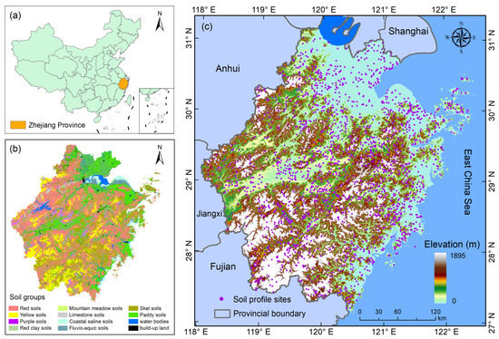
Figure 1.
Study area with locations of soil sampling sites. (a) Location of the study area (Zhejiang Province, China); (b) soil types at the soil group level; and (c) locations of soil profile sites and terrains of the study area.
2.2. Data Sources
A newly available soil database of Zhejiang Province [28,37], providing the most comprehensive and detailed information on Zhejiang soils to date, was used to estimate SOCS in this study. This soil database stores all the basic information including digital soil maps, soil profile sites, soil properties, climate data, terrain, etc. There are six different scales of digital soil maps stored in this soil database, including 1:50,000, 1:250,000, 1:500,000, 1:1,000,000, 1:4,000,000, and 1:10,000,000 (Table 1). The soil map at the scale of 1:4,000,000 was compiled in 1978, while the other five soil maps, which represent soil information in the early 1980s, were compiled during the Second National Soil Survey of China. All these six different scaled soil maps were based on the classification units in the GSCC system. Generally, the classification level of map units decreases as the soil map’s scale increases [19]. The map units of the 1:10,000,000-scale soil map were subgroup and soil group, while the basic map unit of the 1:50,000-scale soil map was soil species. The soils of the 1:50,000-scale soil map were classified into 10 soil groups, 21 subgroups, 99 soil families, and 277 soil species.

Table 1.
Characteristics of the six different scaled soil maps used in this study.
There are 2677 soil profiles stored in this soil database, collected from the Second National Soil Survey of China in the early 1980s. However, no GPS/coordinate records were taken for these soil profiles, having only location descriptions at the village level. Among these 2677 soil profiles, the locations of 2154 soil profile sites were identified according to the descriptions of their locations and environmental conditions and were usually assigned with the central location of the largest polygon related to the same soil type with the soil profile in the village (Figure 1c). These 2154 soil profiles were selected to estimate SOCS in this study. The properties of these soil profiles include extensive information such as soil type name, parent material, soil depth, bulk density, organic matter content, particle composition, and others.
2.3. Methods
2.3.1. Estimation of Soil Organic Carbon Density and Stocks
The soil organic carbon density (SOCD, kg/m2) for each of the 2154 soil profiles was calculated by using the following formula [19,38]:
where n is the number of soil pedogenic layers in the field survey, θi% represents the gravel (>2 mm) content in percent by volume, ρi is the soil bulk density (g/cm3), Ci is the organic carbon content (g/kg) calculated by multiplying the soil organic matter content by 0.58 (the Bemmelen index), and Ti represents the thickness (cm) of the soil pedogenic layer i. SOCD was estimated to have a maximum soil depth of 1 m for comparison purposes with other similar studies. In case the soil pedogenic layer of a soil profile was lacking in some of these properties (e.g., soil bulk density or soil organic matter content), data for the missing soil properties were derived from the mean values of all such soil pedogenic layers of the same soil species or soil family in the same county.
Regional soil organic carbon stock (SOCS, Tg), which represents the total amount of soil organic carbon contained in soils for a given region, was calculated by multiplying the SOCD value for each polygon with the polygon area, and then summing these total values for all polygons for the whole region. The formula was listed as follows:
where n is the number of polygons, SOCDi represents the soil organic carbon density of polygon i, and Ai is the area of polygon i. The SOCS values were calculated based on the 0–1 m soil depth. The mean SOCD value for a region or a soil type was calculated by dividing the total SOCS value by its total area. The SOC estimations were conducted by using ESRI software ArcGIS 10.3 (Redlands, CA, USA), with water bodies and built-up land areas excluded from the calculation.
2.3.2. Methods of Aggregating Soil Profile Data to Represent Map Units
Aggregating soil profile data to represent map units is a preliminary step to calculate regional SOCS and mean SOCD values. The linkage of each soil profile to its corresponding map unit was determined according to the soil type name of this soil profile based on the GSCC system. Then, the SOCD values of soil profiles with the same soil type name were assigned to polygons of the corresponding map unit on a digital soil map by using one of the following three methods: the mean method, the median method, and the pedological professional knowledge-based (PKB) method [19].
Both the mean and median methods were conducted in two stages at the provincial level. First, the SOCD value of each soil type was calculated. Specifically, the arithmetic mean (for the mean method) or median (for the median method) of the SOCD values of all soil profiles with the same soil type name was calculated as the SOCD value of that soil type. Second, the SOCD value of each soil type was linked to all the corresponding polygons of that soil type on a digital soil map. Therefore, different polygons of the same map unit on one soil map were assigned the same SOC density value. Figure 2 shows the procedure of linking SOCD values of soil profiles with their corresponding polygons on a digital soil map using the mean or median method. Different uppercase letters (i.e., A, B, and C) represent different soil types. Uppercase letter with a subsequent Arabic numeral (i) represents the serial number of soil profiles with the same soil type, e.g., A1 represents the No.1 soil profile of soil type A. If a soil type has only one soil profile, the SOCD value of the soil profile will be used to link with all corresponding polygons belonging to that soil type. If a soil type has two or more soil profiles, the arithmetic mean (for the mean method) or the median (for the median method) value was calculated and used for the linkage.
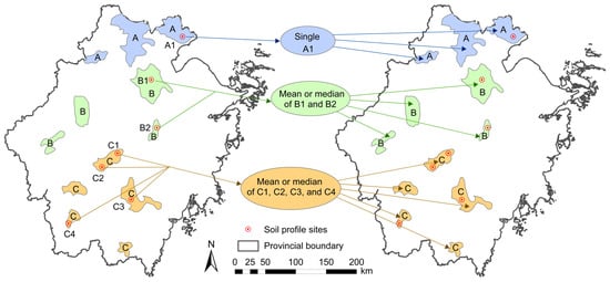
Figure 2.
The procedure of linking SOCD values of soil profiles with their corresponding polygons on a digital soil map using the mean or median method.
The PKB method utilizes multifaceted information about each soil profile, including soil type, parent material, and spatial location. It was conducted at the county level, and therefore, different polygons of the same map unit on a soil map may be assigned different SOCD values. Figure 3 shows the linkage procedure using the PKB method. Different lowercase letters (i.e., a, b, and c) indicate different classes of parent materials related to one soil type, e.g., a1 and a2 represent two classes of parent materials related to soil type A. If a soil type has only one soil profile in a county, the SOCD value of this soil profile was used to link with all corresponding polygons belonging to this soil type in this county. If a soil type has two or more soil profiles in a county, the identity or similarity in parent materials was considered for the linkage, e.g., soil type A has soil profiles of A8 and A9 in Yiwu County, so the SOCD value of A8 was used to link with two polygons with the same parent material class of a1, while the SOCD value of A9 was used to link with the polygon with the parent material class of a2; when two or more soil profiles of one soil type in a county related to the same parent material class, polygons with that parent material class were linked with the SOCD value of the soil profile with the shortest distance, e.g., this rule was applied to the linkage process between polygons and soil profiles of A2 and A3 which had the same soil type A with the same parent material class of a1 in Sheng County; when two or more soil profiles of one soil type were located in one polygon, the arithmetic mean SOCD value was calculated and used to link with that polygon, e.g., this rule was applied to the linkage process between polygons and soil profiles of A5, A6, and A7 which had the same soil type A in Dongyang County.
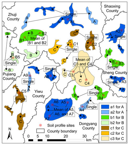
Figure 3.
The procedure of linking SOCD values of soil profiles with their corresponding polygons on a digital soil map using the pedological professional knowledge-based (PKB) method.
2.3.3. Statistical Analysis
The main effects of the map scale and the linkage method on SOC estimations were examined separately by one-way analysis of variance with the Statistical Package for Social Sciences version 20.0 (SPSS Inc., Chicago, IL, USA) for Windows. When a significant (p < 0.05) difference was observed between treatments, then a subsequent Tukey’s test was performed for multiple pairwise comparisons [39]. All spatial analyses including overlay analysis, distance analysis, and zonal statistics were conducted in ArcGIS 10.3.
3. Results
3.1. Scale-Dependence of SOC Dynamics
Figure 4 shows the estimates of SOCS (Figure 4a) and SOCD (Figure 4b) for the study area using the mean, median, and PKB methods based on six different scaled soil maps. Similar increasing trends in the estimates of both SOCS and SOCD were observed for all three linkage methods as the soil map scale decreased from 1:50,000 to 1:10,000,000. The variations in the estimated SOCS and SOCD using soil maps at scales ranging from 1:50,000 to 1:500,000 were generally smaller than those obtained by using soil maps at scales ranging from 1:1,000,000 to 1:10,000,000. The largest differences in the estimates of SOCS and SOCD simultaneously occurred between the 1:500,000-scale soil map and the 1:10,000,000-scale soil map. Compared with the most detailed soil map (i.e., 1:50,000), the estimated SOC values using the mean, median, and PKB methods based on the 1:10,000,000-scale soil map were 10.9%, 5.4%, and 8.4% greater for SOCS, and 14.6%, 8.9%, and 12.0% greater for SOCD, respectively, indicating that the estimates of SOCS and SOCD using small-scale soil maps were often overestimated in Zhejiang Province.
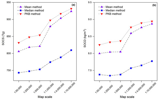
Figure 4.
The estimates of SOCS (a) and SOCD (b) in Zhejiang Province as the soil map scale decreased from 1:50,000 to 1:10,000,000 using the mean, median, and PKB methods.
Significant differences were found in the estimates of both SOCS and SOCD using different linkage methods (Figure 5a), indicating that the linkage process of aggregating soil profile data to represent map units significantly affects SOC estimations. Among the three linkage methods, the estimated SOCS and SOCD values using the PKB method were the highest for all six soil maps, while the estimated SOCS and SOCD values using the median method were significantly lower than those using the PKB and mean methods (Figure 4). As the soil map scale decreased from 1:50,000 to 1:10,000,000, the difference in SOC estimations between the PKB and mean methods decreased, while the difference in SOC estimations between the PKB and median methods increased. The variations of estimated SOCS values for the three linkage methods presented an increasing trend as the soil map scale decreased from 1:50,000 to 1:10,000,000, with a coefficient of variation of 5.7% for the 1:50,000-scale soil map and 7.7% for the 1:10,000,000-scale soil map. This implies that it is important to apply a suitable linkage method for SOC estimation, especially when using small-scale soil maps.
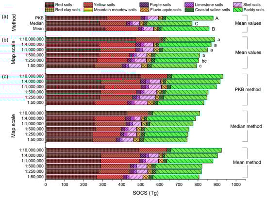
Figure 5.
Effects of the linkage method (a) and the soil map scale (b) on the estimates of SOCS at the soil group level (c). Different uppercase and lowercase letters indicate significant (p < 0.05) differences in the estimated SOCS for different linkage methods (a) and different scaled soil maps (b), respectively.
The results of the one-way analysis of variance presented the differences in the estimates of SOCS using the six different scaled soil maps (Figure 5b). The SOCS values estimated by using the 1:50,000-scale soil map were found to be significantly (p < 0.05) different from those estimated by using soil maps at scales equal to or smaller than 1:500,000, but with no significance compared to the results obtained by using the 1:250,000-scale soil map. The SOCS values estimated by using the 1:500,000-scale soil map were found to be significantly different from those estimated by using soil maps at scales of 1:50,000 or smaller than 1:500,000, but with no significance compared to the 1:250,000-scale soil map. There was no significant difference in the SOC estimations obtained by using the three soil maps at scales of 1:1,000,000, 1:4,000,000, and 1:10,000,000, but significant differences were found in the SOC estimations between soil maps at scales equal to or smaller than 1:1,000,000 and soil maps at scales equal to or greater than 1:500,000.
3.2. Estimates of SOCS at the Soil Group Level
Figure 5c showed the difference in the estimated SOCS at the soil group level using different linkage methods as the soil map scale decreased from 1:50,000 to 1:10,000,000. Compared with the estimated SOCS value (805.88 Tg) using the most detailed 1:50,000-scale soil map with the mean method, the estimated total SOCS values of the study area using soil maps at the scales of 1:250,000 (818.34 Tg), 1:500,000 (821.34 Tg), 1:1,000,000 (879.25 Tg), 1:4,000,000 (903.40 Tg), and 1:10,000,000 (923.74 Tg) were 1.5%, 1.9%, 9.1%, 12.1%, and 14.6% higher than that estimated by using the 1:50,000-scale soil map (Table 2). Such difference could be attributed to the map generalization process, with the added values in total SOCS on the smaller-scale soil map mainly deriving from the conversions from non-soils (e.g., water bodies and built-up land) to soils and from the conversions from soil types of low SOCD values to other soil types of high SOCD values, such as the conversions from Skel Soils (4.89 kg/m2, mean SOCD value of 2154 soil profiles) to Red Soils (6.97 kg/m2, mean SOCD value of 2154 soil profiles).
Table 2.
The estimates of SOCS at the soil group level for the six different scaled soil maps using the mean method.
Large variations in the estimated SOCS values of different soil groups were observed as the soil map scale decreased. There were ten soil groups on the 1:50,000-scale soil map, but only four soil groups (i.e., Red Soils, Yellow Soils, Coastal Saline Soils, and Paddy Soils) were retained on the 1:10,000,000-scale soil map, which indicated that the rest of the six soil groups (i.e., Purple Soils, Limestone Soils, Skel Soils, Red Clay Soils, Mountain Meadow Soils, and Fluvio-aquic Soils) were completely merged into these four retained soil groups. More specifically, the Mountain Meadow Soils and Red Clay Soils were completely merged into other soil groups during the map generalization process as the soil map scale decreased from 1:250,000 to 1:500,000 and from 1:1,000,000 to 1: 4,000,000, respectively, while the Purple Soils, Skel Soils, Limestone Soils, and Fluvio-aquic Soils were completely merged into other soil groups as the soil map scale decreased from 1:4,000,000 to 1:10,000,000. Among the four finally retained soil groups on the 1:10,000,000-scale soil map, the estimated SOCS for Red Soils varied most significantly as the soil map scale decreased from 1:50,000 to 1:10,000,000, with a coefficient of variation of 26.3%. Compared with the estimated SOCS (258.08 Tg, the mean of the three linkage methods) for Red Soils using the 1:50,000-scale soil map, the estimated SOCS for Red Soils using the 1:10,000,000-scale soil map was calculated as 472.06 Tg (the mean of the three linkage methods), with an 82% increase. The added SOCS value (213.98 Tg) for Red Soils during the map generalization process as the soil map scale decreased from 1:50,000 to 1:10,000,000 was mainly derived from the conversions from Skel Soils to Red Soils.
3.3. Spatial Patterns of SOC Estimations
For the analysis of the effects of the soil map scale on the spatial patterns of the SOC estimations, we converted the SOCD maps into geographic vector format obtained by using the six different scaled soil maps as grid maps at a 1 km resolution, and then spatial analysis tools (i.e., Raster Calculator and Zonal Statistics) in ArcGIS were utilized to analyze the spatial differences of SOCD values between the six different scaled soil maps by pairwise comparison. The results are shown in Figure 6.
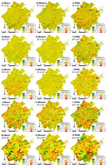
Figure 6.
Spatial variability of the estimated SOCD (kg/m2) values as the soil map scale decreased from 1:50,000 to 1:10,000,000 using the mean, median, and PKB methods. (A–C) represent the spatial variability of SOCD as the soil map scale decreased from 1:50,000 (S1) to 1:250,000 (S2), estimated by using the mean, median, and PKB methods, respectively. (D–O) represent the spatial variability of SOCD as the soil map scale decreased from 1:250,000 (S2) to 1: 500,000 (S3), from 1:500,000 (S3) to 1: 1,000,000 (S4), from 1,000,000 (S4) to 4,000,000 (S5), and from 4,000,000 (S5) to 10,000,000 (S6), respectively.
Generally, the differences in estimated SOCD (i.e., the estimated SOCD using the smaller-scale soil map minus the estimated SOCD using the larger-scale soil map) between two adjacent scaled soil maps were observed showing a decreasing trend as the soil map scale decreased from 1:50,000 to 1:10,000,000. For instance, the differences in estimated SOCD between two adjacent scaled soil maps as the soil map scale decreased from 1:50,000 to 1:10,000,000 using the mean method were calculated as ranging from −100.47 to 90.99 kg/m2, from −89.26 to 33.42 kg/m2, from −31.75 to 32.96 kg/m2, from −29.99 to 17.91 kg/m2, and from −10.91 to 18.03 kg/m2, respectively. However, the percentage of large values (absolute value greater than 5 kg/m2) in the differences of estimated SOCD between two adjacent scaled soil maps was observed to show an increasing trend as the soil map scale decreased from 1:50,000 to 1:10,000,000. This result could be explained by the map generalization process, wherein the generalization intensity increases as the soil map scale decreases. The generalization from the 1:50,000-scale soil map to the 1:250,000-scale soil map was based on the map units at the soil species level, while the generalization from the 1:4,000,000-scale soil map to the 1:10,000,000-scale soil map was based on the map units at the subgroup or soil group level. with four of eight soil groups on the 1:4,000,000-scale soil map eliminated during the map generalization process.
Detailed information on the spatial variability of the estimated SOCD was gradually eliminated as the soil map scale decreased from 1:50,000 to 1:10,000,000, which can be attributed to the larger area of polygons on the smaller-scale soil map during the map generalization process (note that one polygon could only be assigned to one SOCD value, regardless of the soil map scale and the linkage method). The spatial patterns of the differences in estimated SOCD using the three linkage methods presented great differences. The spatial variability of estimated SOCD between two adjacent scaled soil maps from 1:50,000 to 1:500,000 using the mean method was similar to that for the median method, but was markedly different from that for the PKB method. However, the spatial variability of estimated SOCD between two adjacent scaled soil maps from 1:500,000 to 1:10,000,000 using the mean method was markedly different from that for the median method, but was similar to that for the PKB method. This is because the results of aggregating the soil profile data to represent map units for the mean and PKB methods become similar as the soil map scale decreases. The probability of soil profiles belonging to the same map unit located within a single polygon was much higher on the smaller-scale soil maps, and both the mean and PKB methods utilized the mean SOCD value of these soil profiles to link with that polygon. Compared with the mean and median methods, the results obtained from the PKB method could provide more detailed information on the spatial variability of estimated SOCD, especially when using large-scale soil maps, which could be attributed to the difference in the linkage of aggregating soil profile data to represent map units that the PKB method utilizes for multifaceted information of each soil profile, including soil type, parent material, and spatial location.
4. Discussion
4.1. Effects of Map Generalization on SOC Estimations as the Soil Map Scale Decreases
The effects of the soil map scale on SOC estimations mainly resulted from the map generalization process, which is in agreement with the conclusions of previous studies [1,10,19]. One of the most significant changes was that although the mean area of polygons for water bodies and built-up land on a soil map rapidly increased as the soil map scale decreased from 1:50,000 to 1:10,000,000, the total number and total area of polygons for water bodies and built-up land dramatically decreased as the soil map scale decreased (Table 3). There were 3580 polygons for water bodies and 2186 polygons for built-up land on the 1:50,000-scale soil map, but only one polygon for water bodies was retained on the 1:10,000,000-scale soil map, while all the polygons for built-up land were eliminated during the map generalization process. The total area of the retained polygons for water bodies and built-up land on the 1:10,000,000-scale soil map was only 16.8% of that on the 1:50,000-scale soil map, which implied that most polygons for water bodies and built-up land on the 1:50,000-scale soil map were converted into soils during the map generalization process. Such findings were ignored by previous studies, but they are important because the generalization of water bodies and built-up land significantly influence the areas of individual soil types used for the estimates of SOC.
Table 3.
Characteristics of polygons for water bodies and built-up land on the six different scaled soil maps.
The change in the areas of individual soil types caused by the conversion between different soil types was another significant change during the map generalization process (Table 2). We took Red Soils, which had the largest distribution area and SOCS in the study area, as an example of how soil groups changed with the soil map scale. Figure 7 illustrates the effects of the map generalization process for Red Soils on the estimates of SOCS using the mean method. During the map generalization processes, as the soil map scale decreased from 1:50,000 to 1:250,000, from 1:250,000 to 1:500,000, and from 1:500,000 to 1: 1,000,000, respective SOCS values of 198.7 Tg (74.4% of the total estimated SOCS using the 1:50,000-scale soil map), 224.9 Tg (80.0% of the total estimated SOCS using the 1:250,000-scale soil map), and 228.6 Tg (78.5% of the total estimated SOCS using the 1:500,000-scale soil map) for Red Soils were separately retained on the smaller-scale soil map of the two adjacent scaled soil maps, while respective SOCS values of 68.4 Tg (25.6% of the total estimated SOCS using the 1:50,000-scale soil map), 56.4 Tg (20.0% of the total estimated SOCS using the 1:250,000-scale soil map), and 62.6 Tg (21.5% of the total estimated SOCS using the 1:500,000-scale soil map) for Red Soils were separately converted into other soil groups or non-soils on the smaller soil map of the two adjacent scaled soil maps. Compared with the map generalization process as the soil map scale decreased from 1:50,000 to 1:1,000,000, the percentage of retained SOCS values for Red Soils significantly decreased during the map generalization process as the soil map scale decreased from 1:1,000,000 to 10,000,000, indicating that much SOCS for Red Soils were converted into SOCS for other soil groups or non-soils during the map generalization process at small scales.
Figure 7.
Changes in the estimated SOCS (Tg) for Red Soils (soil group) as the soil map scale decreased from 1:50,000 to 1:10,000,000 using the mean method. Each bar represents the estimated SOCS for a soil group and is assigned a unique color at the 1:50,000 scale. The part with its original color in each bar at scales ranging from 1:250,000 to 1:10,000,000 represents the retained SOCS on the smaller-scale soil map during the map generalization process of two adjacent scaled soil maps, while the part with non-original color in each bar represents the converted SOCS deriving from other soil groups or non-soils (i.e., water bodies and built-up land). Waveforms indicate the conversions of SOCS between different soil groups during the map generalization process as the map scale decreased. The two SOCS values (if any) for a soil group listed in the bracket represent the retained and converted parts, respectively.
4.2. Other Factors Influencing SOC Estimations Caused by Different Scales
The number and SOCD values of soil profiles used in the estimates of SOC changed with the changes in the soil map scale. For example, Mountain Meadow Soils were eliminated and completely merged into other soil types on the 1:500,000-scale soil map during the map generalization process as the soil map scale decreased from 1:250,000 to 1:500,000, and all soil profiles belonging to this soil type were excluded from the estimates of SOC. As is shown in Table 4 and Figure 8, the number of soil profiles used for SOC estimations significantly decreased, with 67.0% of them for the mean and median methods and 86.4% of them for the PKB method excluded from the estimation process during the map generalization process as the soil map scale decreased from 1:50,000 to 1:10,000,000. The ranges of SOCD values of the soil profiles presented a decreasing trend as the soil map scale decreased, which resulted from the elimination of soil profiles with extreme SOCD values (i.e., the minimum and maximum values) during the map generalization process. Additionally, the mean SOCD values of soil profiles using the mean and median methods showed an increasing trend during the map generalization process, while no similar trend was observed when using the PKB method, which could be explained by the differences in the linkage procedure between these three methods.
Table 4.
Descriptive statistics of soil profiles used for different scaled soil maps with the mean, median, and PKB methods.
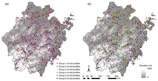
Figure 8.
Changes in soil profiles used for the estimates of SOC as the soil map scale decreased from 1:50,000 to 1:10,000,000 using the mean and median methods (a) and the PKB method (b). Groups 1–5 of the soil profiles represent the soil profiles excluded from the SOC estimations during the map generalization process as the soil map scale decreased from 1:50,000 to 1: 250,000 (group 1), from 1:250,000 to 1: 500,000 (group 2), from 1:500,000 to 1: 1,000,000 (group 3), from 1,000,000 to 4,000,000 (group 4), and from 4,000,000 to 10,000,000 (group 5), respectively. Group 6 of the soil profiles represents the soil profiles used for the 1:10,000,000-scale soil map.
Besides the changes in soil profiles, the linkage method used to aggregate the SOCD values of soil profiles to represent map units also affected the estimates of SOC during the map generalization process. The mean and median methods generally used many more soil profiles than the PKB method during the map generalization process. However, this does not imply that the mean or median method is a better choice for the estimates of SOC compared with the PKB method. The reason is that both the mean and median methods utilized the mean or median SOCD value of all soil profiles belonging to a map unit, which indicated that only one SOCD value was used for one soil type, and all polygons belonging to the same map unit were assigned with the same SOCD value within the whole study area. Such linkage methods did not consider the variation in the SOCD values of soil profiles belonging to the same map unit, which resulted in the elimination of spatial variability in SOCD for the polygons belonging to the same map unit (Figure 6) and increased the uncertainties in the SOC estimations. In contrast, the PKB method utilized multifaceted information (i.e., soil type, parent material, and spatial location) of each soil profile, and different SOCD values of soil profiles belonging to one map unit were linked with corresponding polygons belonging to that same map unit. Therefore, the PKB method could better express the spatial variability in the estimates of SOC, which is more consistent with the regularity of soil distributions in natural environments.
4.3. Implications for Soil Resources Management
The accurate estimate of regional SOCS plays an important role in improving soil quality, dealing with climate change, and formulating reasonable agricultural management [40,41,42]. Our results show that the scale of soil maps directly affects the accuracy of SOC estimation, and that high-resolution soil databases are extremely important for regional SOCS estimations. Thus, the most widely used 1:1,000,000-scale soil map of China is urgently needed to be used instead with a more accurate soil map. This research indicates that the most detailed 1:50,000-scale soil map could serve as the optimal choice for regional SOC estimations in China. However, the 1:50,000 scale digital soil map is unavailable for most regions in China. As an alternative, the 1:500,000 scale digital soil map could be a good choice for regions lacking the 1:50,000-scale soil map because it is easily available and there is little difference between its SOCS estimations and the most detailed 1:50,000-scale soil map.
In addition to the accuracy of regional SOCS estimation, the precise description of its spatial variability is also of great importance. Our results reveal that with the decrease in soil map scale, the ability to characterize the spatial heterogeneity of SOC density significantly decreases. Thus, the most detailed 1:50,000-scale soil map coupled with the PKB method which utilized multifaceted information about each soil profile would be a good choice for regional SOC estimations in China. However, such a soil type method cannot reveal the spatial variations of SOC within polygons. To solve this problem, one feasible approach is the application of remote sensing data with a high spatial resolution to map SOC by building quantitative soil–landscape models [1,43,44,45,46,47].
4.4. Advantages and Limitations of Our Study
Our results accord with other previous works on evaluating the effects of the soil map scale on SOCS estimations, which found that the scale of the soil map significantly influences the accurate estimates of SOC at a regional scale [1,10,14,19,20,21,30,48]. Compared with these previous works, our study found that in addition to the conversion between different soil types, the conversion from non-soils (i.e., water bodies and built-up land) to soils during the map generalization process also served as one of the most crucial factors affecting the estimates of SOC, which was ignored by previous studies. Additionally, the linkage method was also found to significantly impact the estimates of SOC at different soil map scales. We quantified the changes in the number and SOCD values of soil profiles during the map generalization process and revealed the process of how different linkage methods aggregated the SOCD values of soil profiles to represent map units as the soil map scale decreased from 1:50,000 to 1:10,000,000. Moreover, the effects of different linkage methods on the spatial variability of SOCD estimated by using different scaled soil maps were determined.
Although our research has made some progress as mentioned above, there are certain shortcomings. First, due to the unavailability of data, the evaluation of soil maps at a scale larger than 1:50,000 derived from the Second National Soil Survey of China could not be conducted. Second, soil profiles were taken from the Second National Soil Survey of China in the early 1980s, which did not have GPS/coordinate records. The locations of soil profile sites used in this study were identified according to the descriptions of their locations and environmental conditions, but the deviation between the actual locations and the locations of our results may lead to uncertainty in the SOC estimations. Therefore, new national soil surveys are needed to obtain reliable up-to-date soil information in China. In addition, recent publications indicate that digital soil mapping models, which build quantitative soil–landscape relationships using soil sampling data and relevant environmental variables (e.g., climate, remote sensing imagery, and terrain), have demonstrated excellent capabilities in mapping soil classes/properties at scales from the global to the field level in the past decade [49,50,51,52,53]. Therefore, the comparison of soil-map-based linkage methods with digital soil mapping methods regarding their influence on SOC estimations deserves further study and exploration.
5. Conclusions
This study analyzed the effects of the soil map scale on the estimates of SOC in southeastern China. Specifically, this study focused on revealing the process of how different linkage methods aggregated soil profile data to represent map units, which directly impacted the spatial variability of the SOC estimations during the map generalization process as the soil map scale decreased from 1:50,000 to 1:10,000,000. Our results demonstrated that both the soil map scale and the linkage method were of crucial importance for regional SOC estimations, and their influences on the differences in estimated SOC could be attributed to the changes in the number of soil profiles, the conversions between different soil types, the conversions from non-soils (i.e., water bodies and built-up land) to soils, and the linkage methods of aggregating the SOCD values of soil profiles to represent map units during the map generalization process. From the view of pedogenesis, not only the estimated SOCS but also its spatial variability across the study area should be considered in the estimates of SOC; thus, the most detailed 1:50,000-scale soil map, coupled with the PKB method which utilized multifaceted information (i.e., soil type, parent material, and spatial location) of each soil profile, serves as a good choice for regional SOC estimations in China. This can be applied as a reference for developing soil management strategies and coping with future climate change.
Author Contributions
Conceptualization, J.Z.; methodology, J.Z.; software, X.C., E.W., Y.Z., L.W. and L.Q.; validation, J.Z.; formal analysis, J.Z. and L.Q.; investigation, X.C. and J.Z.; resources, J.W.; data curation, J.W.; writing—original draft preparation, J.Z.; writing—review and editing, J.Z.; visualization, X.C., E.W., Y.Z., L.W. and L.Q.; supervision, J.W.; project administration, J.Z. and J.W.; funding acquisition, J.Z. and J.W. All authors have read and agreed to the published version of the manuscript.
Funding
This research was funded by the MOE (Ministry of Education in China) Youth Foundation Project of Humanities and Social Sciences (Grant No. 21YJCZH243).
Institutional Review Board Statement
Not applicable.
Informed Consent Statement
Not applicable.
Data Availability Statement
Not applicable.
Conflicts of Interest
The authors declare no conflict of interest.
Appendix A
Table A1.
Reference conversions between soil groups of the GSCC (Genetic Soil Classification of China) system and Soil Order of the U.S. Taxonomy and WRB (World Reference Base for soil resources) soil groups.
Table A1.
Reference conversions between soil groups of the GSCC (Genetic Soil Classification of China) system and Soil Order of the U.S. Taxonomy and WRB (World Reference Base for soil resources) soil groups.
| Soil Groups of GSCC | Number of Soil Profiles | Soil Order of U.S. Taxonomy | WRB Soil Groups |
|---|---|---|---|
| Red Soils | 372 | Alfisols, Ultisols, Inceptisols | Cambisols |
| Yellow Soils | 126 | Alfisols, Inceptisols | Cambisols |
| Purple Soils | 84 | Inceptisols, Entisols | Cambisols |
| Limestone Soils | 22 | Mollisols, Inceptisols | Cambisols |
| Skel Soils | 114 | Inceptisols, Entisols | Regosols |
| Red Clay Soils | 4 | Inceptisols, Alfisols | Cambisols |
| Mountain Meadow Soils | 4 | Histosols, Inceptisols | Cambisols |
| Fluvio-aquic Soils | 189 | Inceptisols, Entisols | Cambisols |
| Coastal Saline Soils | 64 | Inceptisols | Solonchaks |
| Paddy Soils | 1175 | Anthrosols | Anthrosols |
References
- Zhang, L.; Liu, Y.; Li, X.; Huang, L.; Yu, D.; Shi, X.; Chen, H.; Xing, S. Effects of soil map scales on simulating soil organic carbon changes of upland soils in Eastern China. Geoderma 2018, 312, 159–169. [Google Scholar] [CrossRef]
- Silatsa, F.B.T.; Yemefack, M.; Tabi, F.O.; Heuvelink, G.B.M.; Leenaars, J.G.B. Assessing countrywide soil organic carbon stock using hybrid machine learning modelling and legacy soil data in Cameroon. Geoderma 2020, 367, 114260. [Google Scholar] [CrossRef]
- Tan, W.; Zhang, R.; Cao, H.; Huang, C.; Yang, Q.; Wang, M.; Koopal, L.K. Soil inorganic carbon stock under different soil types and land uses on the Loess Plateau region of China. Catena 2014, 121, 22–30. [Google Scholar] [CrossRef]
- Hein, C.J.; Usman, M.; Eglinton, T.I.; Haghipour, N.; Galy, V.V. Millennial-scale hydroclimate control of tropical soil carbon storage. Nature 2020, 581, 63–66. [Google Scholar] [CrossRef] [PubMed]
- Wu, J.; Zhang, H.; Pan, Y.; Krause-Jensen, D.; He, Z.; Fan, W.; Xiao, X.; Chung, I.; Marbà, N.; Serrano, O.; et al. Opportunities for blue carbon strategies in China. Ocean Coast. Manag. 2020, 194, 105241. [Google Scholar] [CrossRef]
- Gentile, R.M.; Malepfane, N.M.; van den Dijssel, C.; Arnold, N.; Liu, J.; Müller, K. Comparing deep soil organic carbon stocks under kiwifruit and pasture land uses in New Zealand. Agric. Ecosyst. Environ. 2021, 306, 107190. [Google Scholar] [CrossRef]
- Guo, P.; Li, M.; Luo, W.; Tang, Q.; Liu, Z.; Lin, Z. Digital mapping of soil organic matter for rubber plantation at regional scale: An application of random forest plus residuals kriging approach. Geoderma 2015, 237–238, 49–59. [Google Scholar] [CrossRef]
- Dos Santos, C.C.; Souza De Lima Ferraz Junior, A.; Oliveira Sá, S.; Andrés Muñoz Gutiérrez, J.; Braun, H.; Sarrazin, M.; Brossard, M.; Desjardins, T. Soil carbon stock and Plinthosol fertility in smallholder land-use systems in the eastern Amazon, Brazil. Carbon Manag. 2018, 9, 655–664. [Google Scholar] [CrossRef]
- Xu, L.; Yu, G.; He, N. Increased soil organic carbon storage in Chinese terrestrial ecosystems from the 1980s to the 2010s. J. Geogr. Sci. 2019, 29, 49–66. [Google Scholar] [CrossRef] [Green Version]
- Xu, S.; Zhao, Y.; Shi, X.; Yu, D.; Li, C.; Wang, S.; Tan, M.; Sun, W. Map scale effects of soil databases on modeling organic carbon dynamics for paddy soils of China. Catena 2013, 104, 67–76. [Google Scholar] [CrossRef]
- Gristina, L.; Scalenghe, R.; García Díaz, A.; Matranga, M.G.; Ferraro, V.; Guaitoli, F.; Novara, A. Soil organic carbon stocks under recommended management practices in different soils of semiarid vineyards. Land Degrad. Dev. 2020, 31, 1906–1914. [Google Scholar] [CrossRef]
- Paustian, K.; Lehmann, J.; Ogle, S.; Reay, D.; Robertson, G.P.; Smith, P. Climate-smart soils. Nature 2016, 532, 49–57. [Google Scholar] [CrossRef] [Green Version]
- Wang, S.; Xu, L.; Zhuang, Q.; He, N. Investigating the spatio-temporal variability of soil organic carbon stocks in different ecosystems of China. Sci. Total Environ. 2021, 758, 143644. [Google Scholar] [CrossRef] [PubMed]
- Galbraith, J.M.; Kleinman, P.J.A.; Bryant, R.B. Sources of Uncertainty Affecting Soil Organic Carbon Estimates in Northern New York. Soil Sci. Soc. Am. J. 2003, 67, 1206–1212. [Google Scholar] [CrossRef]
- Yu, D.; Ni, Y.; Shi, X.; Wang, N.; Warner, E.; Liu, Y.; Zhang, L. Optimal Soil Raster Unit Resolutions in Estimation of Soil Organic Carbon Pool at Different Map Scales. Soil Sci. Soc. Am. J. 2014, 78, 1079–1086. [Google Scholar] [CrossRef]
- Li, L.; Burger, M.; Du, S.; Zou, W.; You, M.; Hao, X.; Lu, X.; Zheng, L.; Han, X. Change in soil organic carbon between 1981 and 2011 in croplands of Heilongjiang Province, northeast China. J. Sci. Food Agric. 2016, 96, 1275–1283. [Google Scholar] [CrossRef]
- Zhao, M.; Qiu, S.; Wang, S.; Li, D.; Zhang, G. Spatial-temporal change of soil organic carbon in Anhui Province of East China. Geoderma Reg. 2021, 26, e415. [Google Scholar] [CrossRef]
- Batjes, N.H. Total carbon and nitrogen in the soils of the world. Eur. J. Soil Sci. 2014, 65, 10–21. [Google Scholar] [CrossRef]
- Zhao, Y.; Shi, X.; Weindorf, D.C.; Yu, D.; Sun, W.; Wang, H. Map Scale Effects on Soil Organic Carbon Stock Estimation in North China. Soil Sci. Soc. Am. J. 2006, 70, 1377–1386. [Google Scholar] [CrossRef]
- Chen, Z.; Zhang, N.; Zhang, L.; Yuan, P.; Yao, C.; Xing, S.; Qiu, L.; Chen, H.; Fan, X. Scale effects of estimation of soil organic carbon storage in Fujian Province, China. Acta Pedol. Sin. 2018, 55, 606–619. [Google Scholar]
- Zhong, B.; Xu, Y. Scale Effects of Geographical Soil Datasets on Soil Carbon Estimation in Louisiana, USA: A Comparison of STATSGO and SSURGO. Pedosphere 2011, 21, 491–501. [Google Scholar] [CrossRef]
- Yu, D.; Pan, Y.; Zhang, H.; Wang, X.; Ni, Y.; Zhang, L.; Shi, X. Equality testing for soil grid unit resolutions to polygon unit scales with DNDC modeling of regional SOC pools. Chin. Geogr. Sci. 2017, 27, 552–568. [Google Scholar] [CrossRef]
- Illiger, P.; Schmidt, G.; Walde, I.; Hese, S.; Kudrjavzev, A.E.; Kurepina, N.; Mizgirev, A.; Stephan, E.; Bondarovich, A.; Frühauf, M. Estimation of regional soil organic carbon stocks merging classified land-use information with detailed soil data. Sci. Total Environ. 2019, 695, 133755. [Google Scholar] [CrossRef] [PubMed]
- Lorenzetti, R.; Barbetti, R.; Fantappiè, M.; L’Abate, G.; Costantini, E.A.C. Comparing data mining and deterministic pedology to assess the frequency of WRB reference soil groups in the legend of small scale maps. Geoderma 2015, 237–238, 237–245. [Google Scholar] [CrossRef]
- Ma, D.; Zhang, H.; Song, X.; Xing, S.; Fan, M.; Heiling, M.; Liu, L.; Zhang, L.; Mao, Y. Estimating soil organic carbon and nitrogen stock based on high-resolution soil databases in a subtropical agricultural area of China. Soil Tillage Res. 2022, 219, 105321. [Google Scholar] [CrossRef]
- Rasaei, Z.; Rossiter, D.G.; Farshad, A. Rescue and renewal of legacy soil resource inventories in Iran as an input to digital soil mapping. Geoderma Reg. 2020, 21, e262. [Google Scholar] [CrossRef]
- Sulaeman, Y.; Minasny, B.; McBratney, A.B.; Sarwani, M.; Sutandi, A. Harmonizing legacy soil data for digital soil mapping in Indonesia. Geoderma 2013, 192, 77–85. [Google Scholar] [CrossRef]
- Zhi, J.; Jing, C.; Lin, S.; Zhang, C.; Wu, J. Estimates of Soil Organic Carbon Stocks in Zhejiang Province of China Based on 1:50 000 Soil Database Using the PKB Method. Pedosphere 2015, 25, 12–24. [Google Scholar] [CrossRef]
- Li, W.; Jia, S.; He, W.; Raza, S.; Zamanian, K.; Zhao, X. Analysis of the consequences of land-use changes and soil types on organic carbon storage in the Tarim River Basin from 2000 to 2020. Agric. Ecosyst. Environ. 2022, 327, 107824. [Google Scholar] [CrossRef]
- Zhang, L.; Zhuang, Q.; Zhao, Q.; He, Y.; Yu, D.; Shi, X.; Xing, S. Uncertainty of organic carbon dynamics in Tai-Lake paddy soils of China depends on the scale of soil maps. Agric. Ecosyst. Environ. 2016, 222, 13–22. [Google Scholar] [CrossRef]
- Shangguan, W.; Dai, Y.; Liu, B.; Ye, A.; Yuan, H. A soil particle-size distribution dataset for regional land and climate modelling in China. Geoderma 2012, 171–172, 85–91. [Google Scholar] [CrossRef]
- Liang, Z.; Chen, S.; Yang, Y.; Zhao, R.; Shi, Z.; Viscarra Rossel, R.A. National digital soil map of organic matter in topsoil and its associated uncertainty in 1980’s China. Geoderma 2019, 335, 47–56. [Google Scholar] [CrossRef]
- Liang, Z.; Chen, S.; Yang, Y.; Zhou, Y.; Shi, Z. High-resolution three-dimensional mapping of soil organic carbon in China: Effects of SoilGrids products on national modeling. Sci. Total Environ. 2019, 685, 480–489. [Google Scholar] [CrossRef] [PubMed]
- Wang, D.; Yan, Y.; Li, X.; Shi, X.; Zhang, Z.; Weindorf, D.C.; Wang, H.; Xu, S. Influence of climate on soil organic carbon in Chinese paddy soils. Chin. Geogr. Sci. 2017, 27, 351–361. [Google Scholar] [CrossRef]
- Shi, X.; Yu, D.; Xu, S.; Warner, E.; Wang, H.; Sun, W.; Zhao, Y.; Gong, Z. Cross-reference for relating Genetic Soil Classification of China with WRB at different scales. Geoderma 2010, 155, 344–350. [Google Scholar] [CrossRef]
- Zhi, J.; Jing, C.; Lin, S.; Zhang, C.; Liu, Q.; DeGloria, S.D.; Wu, J. Estimating soil organic carbon stocks and spatial patterns with statistical and GIS-based methods. PLoS ONE 2014, 9, e97757. [Google Scholar] [CrossRef]
- Wu, J.Y.H.; Zhi, J.; Jing, C.; Chen, H.; Xu, J.; Lin, S.; Li, D.; Zhang, C.; Xiao, R.; Huang, H. A 1:50000 scale soil database of Zhejiang Province, China. Acta Pedol. Sin. 2013, 50, 30–40. [Google Scholar]
- Morisada, K.; Ono, K.; Kanomata, H. Organic carbon stock in forest soils in Japan. Geoderma 2004, 119, 21–32. [Google Scholar] [CrossRef]
- Albaladejo, J.; Ortiz, R.; Garcia-Franco, N.; Navarro, A.R.; Almagro, M.; Pintado, J.G.; Martínez-Mena, M. Land use and climate change impacts on soil organic carbon stocks in semi-arid Spain. J. Soils Sediments 2013, 13, 265–277. [Google Scholar] [CrossRef]
- Du, H.; Wang, T.; Xue, X.; Li, S. Estimation of soil organic carbon, nitrogen, and phosphorus losses induced by wind erosion in Northern China. Land Degrad. Dev. 2019, 30, 1006–1022. [Google Scholar] [CrossRef]
- Mikhailova, E.A.; Altememe, A.H.; Bawazir, A.A.; Chandler, R.D.; Cope, M.P.; Post, C.J.; Stiglitz, R.Y.; Zurqani, H.A.; Schlautman, M.A. Comparing soil carbon estimates in glaciated soils at a farm scale using geospatial analysis of field and SSURGO data. Geoderma 2016, 281, 119–126. [Google Scholar] [CrossRef] [Green Version]
- Zhou, Y.; Chartin, C.; Van Oost, K.; van Wesemael, B. High-resolution soil organic carbon mapping at the field scale in Southern Belgium (Wallonia). Geoderma 2022, 422, 115929. [Google Scholar] [CrossRef]
- Hengl, T.; de Jesus, J.M.; MacMillan, R.A.; Batjes, N.H.; Heuvelink, G.B.; Ribeiro, E.; Samuel-Rosa, A.; Kempen, B.; Leenaars, J.G.; Walsh, M.G.; et al. SoilGrids1km--global soil information based on automated mapping. PLoS ONE 2014, 9, e105992. [Google Scholar] [CrossRef] [Green Version]
- Hengl, T.; Miller, M.A.E.; Križan, J.; Shepherd, K.D.; Sila, A.; Kilibarda, M.; Antonijević, O.; Glušica, L.; Dobermann, A.; Haefele, S.M.; et al. African soil properties and nutrients mapped at 30 m spatial resolution using two-scale ensemble machine learning. Sci. Rep. 2021, 11, 6130. [Google Scholar] [CrossRef] [PubMed]
- Hengl, T.; Nussbaum, M.; Wright, M.N.; Heuvelink, G.B.M.; Gräler, B. Random forest as a generic framework for predictive modeling of spatial and spatio-temporal variables. PeerJ 2018, 6, e5518. [Google Scholar] [CrossRef] [Green Version]
- Gupta, S.; Papritz, A.; Lehmann, P.; Hengl, T.; Bonetti, S.; Or, D. Global mapping of soil water characteristics parameters—Fusing curated data with machine learning and environmental covariates. Remote Sens. 2022, 14, 1947. [Google Scholar] [CrossRef]
- Guevara, M.; Arroyo, C.; Brunsell, N.; Cruz, C.O.; Domke, G.; Equihua, J.; Etchevers, J.; Hayes, D.; Hengl, T.; Ibelles, A.; et al. Soil organic carbon across Mexico and the conterminous United States (1991–2010). Glob. Biogeochem. Cycles 2020, 34, e2019GB006219. [Google Scholar] [CrossRef]
- Li, X.; Wang, S.; Zhang, L.; Yu, D.; Shi, X.; Li, J.; Xing, S.; Wang, G. Impacts of source of soil data and scale of mapping on assessment of organic carbon storage in upland soil. Acta Pedol. Sin. 2016, 53, 58–71. [Google Scholar]
- Hengl, T.; Heuvelink, G.B.M.; Kempen, B.; Leenaars, J.G.B.; Walsh, M.G.; Shepherd, K.D.; Sila, A.; MacMillan, R.A.; Mendes De Jesus, J.; Tamene, L.; et al. Mapping soil properties of Africa at 250 m resolution: Random Forests significantly improve current predictions. PLoS ONE 2015, 10, e125814. [Google Scholar]
- Hengl, T.; Toomanian, N.; Reuter, H.I.; Malakouti, M.J. Methods to interpolate soil categorical variables from profile observations: Lessons from Iran. Geoderma 2007, 140, 417–427. [Google Scholar] [CrossRef]
- Ramcharan, A.; Hengl, T.; Nauman, T.; Brungard, C.; Waltman, S.; Wills, S.; Thompson, J. Soil property and class maps of the conterminous United States at 100-meter spatial resolution. Soil Sci. Soc. Am. J. 2018, 82, 186–201. [Google Scholar] [CrossRef] [Green Version]
- Das, B.; Rathore, P.; Roy, D.; Chakraborty, D.; Jatav, R.S.; Sethi, D.; Kumar, P. Comparison of bagging, boosting and stacking algorithms for surface soil moisture mapping using optical-thermal-microwave remote sensing synergies. Catena 2022, 217, 106485. [Google Scholar] [CrossRef]
- Wadoux, A.M.J.; Molnar, C. Beyond prediction: Methods for interpreting complex models of soil variation. Geoderma 2022, 422, 115953. [Google Scholar] [CrossRef]
Publisher’s Note: MDPI stays neutral with regard to jurisdictional claims in published maps and institutional affiliations. |
© 2022 by the authors. Licensee MDPI, Basel, Switzerland. This article is an open access article distributed under the terms and conditions of the Creative Commons Attribution (CC BY) license (https://creativecommons.org/licenses/by/4.0/).