Article

Conservation and Development: Spatial Identification of Relative Poverty Areas Affected by Protected Areas in China and Its Spatiotemporal Evolutionary Characteristics

1
Department of Landscape Architecture, School of Architecture, Tsinghua University, Beijing 100084, China
2
Department of Architecture, School of Architecture, Tsinghua University, Beijing 100084, China
3
Institute for National Parks, Tsinghua University, Beijing 100084, China
*
Author to whom correspondence should be addressed.
Land 2022, 11(7), 1048; https://doi.org/10.3390/land11071048
Submission received: 7 June 2022 / Revised: 7 July 2022 / Accepted: 7 July 2022 / Published: 11 July 2022
(This article belongs to the Section Land Environmental and Policy Impact Assessment)

Abstract

:
Currently, biodiversity conservation and the achievement of common prosperity are important challenges. China bid farewell to “absolute poverty” in 2020 but continues to face challenges, such as relative multidimensional poverty, especially in regions of protected areas (PA). The correlation between poverty and the natural environment leads to further research on the distribution and spatiotemporal evolutionary characteristics of relative poverty regions affected by the restrictive policies of PA. Quantitative research on these regions helps researchers formalize ecological indemnification policies based on the condition of different regions, thereby stabilizing efforts toward poverty alleviation. Through a study on relative poverty areas in 489 county-level administrative regions in China influenced by 477 national nature reserves, this study formulated a multidimensional integrated poverty index model that comprises three systems, namely, natural environment, economy, and society and 13 indicators. Using the comprehensive index, spatial analysis, and cluster analysis to investigate the evolutionary characteristics and driving factors of poverty from 2014 to 2019, the study created a distribution map of relative poverty regions affected by PA. The results indicated the following. (i) Relative poverty regions are mainly concentrated in provinces on the northwest side of the Hu Line with strong spatial correlation between these regions. Among them, the relatively poor areas with persistent deterioration become the keystone to stabilizing poverty alleviation and promoting green development. (ii) Poverty alleviation focuses on the economic dimension, whereas the environmental and social dimensions lack engagement. (iii) Conservation areas overlap with relative poverty regions. However, the increase in PA does not necessarily lead to the aggravation of the poverty in counties. The results offer a valuable reference for decision makers in formulating targeted policies and measures for areas affected by PA to facilitate green development and common prosperity.

1. Introduction

Environmental conservation and poverty eradication are important goals of global sustainable development in the 21st century. Since the “United Nations (UN) World Summit on Sustainable Development” in 1992 and “UN Conference on Environment and Development” in 2002, balancing conservation and poverty reduction has become the focus of global academic topics [1,2]. Due to the inherent correlation between poverty and ecology [3,4], poor areas in developing countries are overlapping with protected areas (PA), including potential PA [5]. The restrictive conservation policies of PA are a double-edged sword as conservation and development are conflicting yet congruous [6,7].
Recently, the ecological environment in China has significantly improved [8], as the country bid farewell to “absolute poverty” in 2020. Furthermore, schemes for ecological poverty alleviation and green development that were widely administered on PA have demonstrated favorable outcomes. However, communities affected by the restrictive management policies of PA may continue to experience “relative poverty” or “multidimensional poverty,” such as the limited utilization of ecological resources, weak economy structure and transportation infrastructure, limited access to information, and unsophisticated social culture [9]. Such scenarios hinder the sustainable development of these regions or even risk the chances of poverty rising again. Therefore, it is crucial to understand the overall situation of poverty alleviation in these areas before further formulating policies to enhance and stabilize the existing efforts to reduce poverty and promote green development. The foundation of the study is laid on quantitative research on spatial distribution patterns and the spatiotemporal evolutionary characteristics of relative poverty areas affected by PA, taking differentiated measures to stabilize the existing efforts of ecological poverty alleviation and to scientifically formulate green development policies to achieve common prosperity in the new era is of great significance.
Hitherto, studies on poverty measurement in China comprise of geographic identification [10], poverty typology [11], spatial and temporal evolution and heterogeneity [12], driving mechanisms of poverty [13], paths of poverty alleviation, and policy recommendations [14]. The multidimensional poverty measure is a scientific method use in identifying regional poverty and unraveling the poverty situation across regions [15], reflecting the holistic situation of poverty while providing an accurate depiction of the dynamic evolution compared with a single economic income dimension. According to Sen’s theory of “capability poverty” [16], poverty is the deprivation of basic human capabilities, and poverty indicators cover various capability factors such as economic income and level of education. Based on Sen’s theory, the UN Human Development Report (HDR) adopts the Human Development Index (HDI) to evaluate the combined achievements of a country or region’s human development in the three dimensions of “health, knowledge, and living level”. In addition, some researchers have validated that rural poverty in China is related to factors such as geographic location, natural environment, and primary infrastructure [17,18]. In order to integrate multidimensional poverty indicators, methodologies such as HDI [19] and Multidimensional Poverty Indexes (MPI) [9,20] are utilized based on different scales of geographical location and unit of measurement.
Although several studies explored the relation between conservation and poverty [21,22], studies on poverty continue to lack a focus on PA. The total land area of the nature reserve in China accounts for 14.8% of the country’s land area, which makes it a country with a large area of nature reserves in the world [23]. However, few empirical studies use appropriate data and methods to accurately measure the distribution of relative multidimensional poverty areas affected by PA. Moreover, studies discussing the impact of reserve size on poverty are scarce. The recent policies on poverty alleviation and sustainable development in China, such as the “common prosperity” scheme, emphasize the comprehensive consideration of social and economic development and environmental conservation. However, systematic discussions and quantitative research on the degree and causation of relative poverty and current development status of relative poverty regions affected by PA remain lacking.
Based on the discussed context and given the spatial heterogeneity and correlation of PA communities, this study adopted county-level administrative regions influenced by national nature reserves (NNR) in China as the research subject. Moreover, the study formulated an evaluation framework of the Multidimensional Comprehensive Poverty Index to fully understand the comprehensive and multidimensional poverty status of PA regions. The objectives of the study are as follows:
  • To present the spatial distribution pattern and its spatiotemporal evolution characteristics of relative poverty regions affected by PA from 2014 to 2019, and identify key areas that require enhancement in the quality of poverty eradication for the future.
  • To determine the driving factors of the degree of poverty, especially those relative to poverty communities of PA.
  • To explore the correlation between the scale of PA and the degree of poverty in China.
This study provides data references and policy suggestions for the scientific optimization of strategies for ecological poverty alleviation, green development plans, and the differentiated schemes used to achieve common prosperity.

2. Materials and Methods
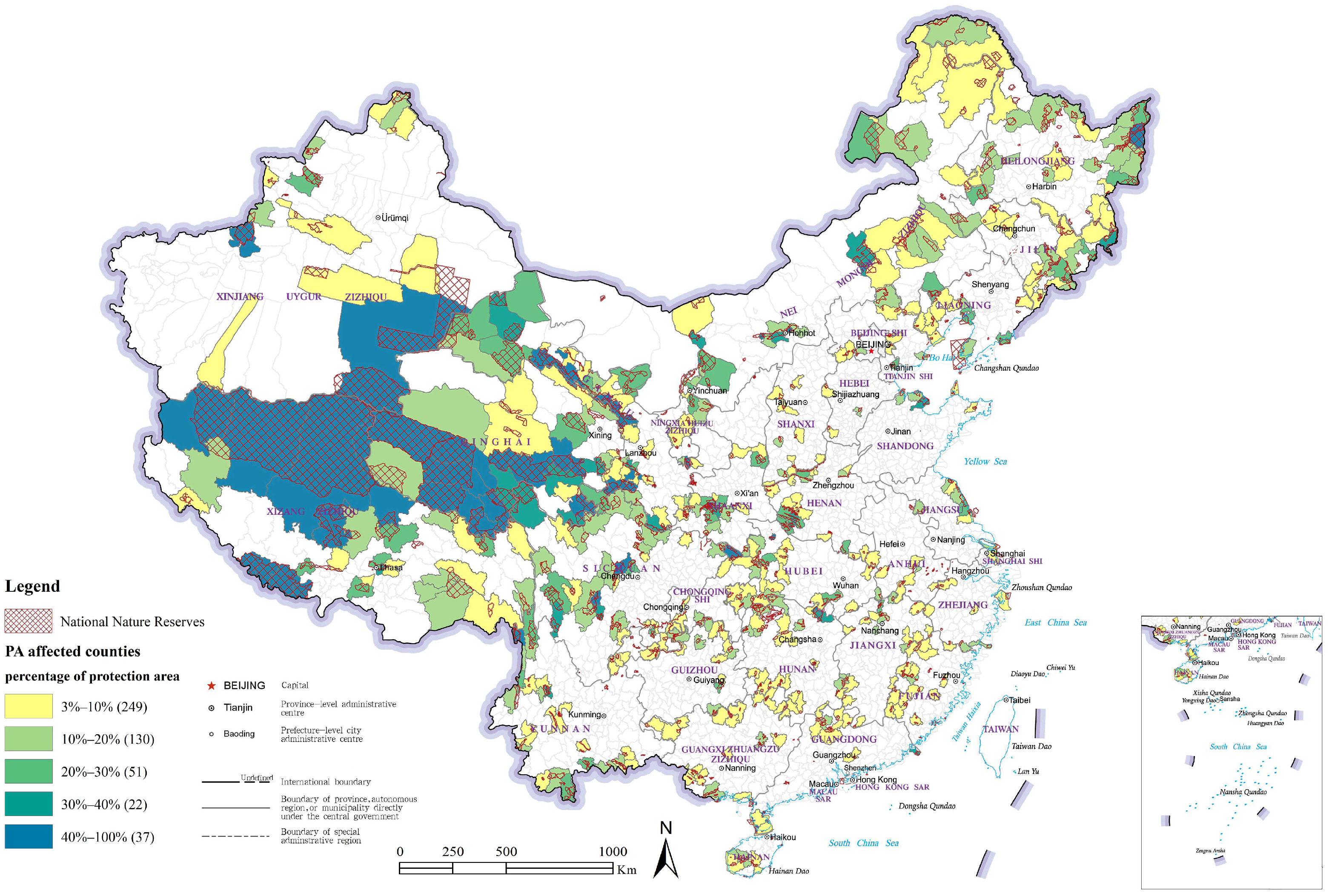
2.1. Study Area

Nature reserves in China, as the largest and oldest type of PA, exert an extensive and profound influence on their surroundings. Among them, the NNR implement the highest level of protection and most stringent conservation management (similar to the newly established national parks in China). As of 31 December 2021, the number of NNR was 477 with a total area of more than one million km2 and involved at least 544 county-level administrative regions in China (Taiwan Province, Hong Kong, and Macau are excluded from this study owing to difficulties in obtaining data). According to the Outline for Poverty Alleviation and Development in Rural China (2011–2020), which was implemented in 2011, the number of poverty-stricken counties in China 832, out of which more than 50% of the counties (excluding urban districts) influenced by NNR are previously national poverty-stricken counties. Considering the possible imprecision in defining the PA boundary and temporal impact of its formation, this study screened 489 county-level administrative regions that comprise PA formed prior to 2011 and cover more than 3% of restrictive protection areas (Figure 1).
A total of 249, 130, 51, and 59 counties possess 3–10%, 10–20%, 20–30%, and more than 30% of the PA, respectively. Typically, each county may also have provincial and municipal nature reserves or other types of PA, such as scenic spots and forest parks.

2.2. Data

This study analyzed relative poverty regions of NNR in 2014 and 2019 using spatial data and socioeconomic statistics. The data sources are as follows.
  • NNR and its administrative district boundary data. The data of 477 NNR boundaries were provided by the “Resource and Environment Science and Data Center” (https://www.resdc.cn/data.aspx?DATAID=272 [accessed on 1 May 2021]) of the Institute of Geographical Sciences and Natural Resources Research, Chinese Academy of Sciences (CAS). The administrative district boundary vector map was obtained from National Geomatics Center of China (https://www.ngcc.cn [accessed on 1 May 2021]). The base map is from Ministry of Natural Resources of the People’s Republic of China (http://bzdt.ch.mnr.gov.cn/ [accessed on 4 July 2022]).
  • Natural environment data. The digital elevation model (250 m resolution) and China’s annual vegetation index (NDVI) datasets (1 km resolution) on spatial distribution were obtained from the Data Center for Resource and Environmental Sciences of the CAS. The cropland area was extracted from land cover classification gridded maps (300 m resolution) offered by the European Space Agency Climate Change Initiative (http://www.esa-landcover-cci.org/ [accessed on 1 May 2021]).
  • Socioeconomic statistics. The data were mainly collated from the China County Statistical Yearbook (2015 and 2020) and partially supplemented by the statistical yearbooks of provinces and cities and their national economic and social development statistical bulletins. Several missing data were interpolated using the mean replacement and multiple substitution methods.
  • Nighttime light data. The study employed the nighttime data provided by the WIND database of Jagger Wangyan Space Vision (https://www.wywxdata.cn/index.html#product [accessed on 1 May 2021]). These data are based on the monthly nighttime light raster remote sensing images collected by NPP-VIIRS and Loyola 1 star. The original images went through a series of denoising, fitting, and calibration and generated the average value of annual nighttime light intensity of county-level administrative units which reflects the intensity of regional human activities.
All spatial data were put through Albers projection, which is an equal area conic projection to standardize all spatial resolution to 1 km in ArcGIS 10.2. The average value of each county was extracted by the zonal statistics operation. In addition, the range method was adopted to normalize the raw data from 2014 and 2019 within the same matrix, hence ensuring the comparability of the poverty index and reducing the dimensional impact across time on it. This makes the poverty index in 2014 and 2019 more significant and the difference in value change more apparent.

2.3. Methods

2.3.1. Indicator Framework of the Comprehensive Poverty Measurement of County-Level Poverty

(1)
Indicator framework
The county level poverty indicator framework is different from that of the population’s. While the population poverty indicator framework focuses on whether individual’s behavioral capacity is deprived, the county level poverty measurement focuses more on the regional sustainable development capacity. Therefore, this paper believes that the county poverty measurement analysis should regard the economy, society, and natural environment as three equally important subsystems. The sustainability indicators of economic development, human (social) development, and natural environmental status of poor counties are respectively reflected in a gradual and progressive systematic framework [9]. On this basis, the HDI method was used to comprehensively characterize the average poverty level of the three subsystems in the county. The framework of the comprehensive poverty measurement indicator reflects the ability of a region to implement sustainable development, which involves three dimensions, namely, economy, society, and natural environments. Referring to the indicator framework of other scholars [13,24] combined with the core monitoring indicators of poverty alleviation in poor counties and considering the principles of availability and scientifically supported indicators, the current study constructed an indicator framework for multidimensional poverty measurement based on 13 indicators across the three dimensions. Furthermore, the indicators were classified into positive and negative (Table 1). The environment dimension sets the foundation for regional poverty alleviation because it comprises ecological environment and resource endowment, which is reflected through indicators, such as percentage of land area with slopes at >15°, elevation, NDVI, and per capita cultivated land area. The economic dimension refers to financial capital and reflects the degree of poverty in economic development and performance in poverty alleviation through indicators, such as per capita output value, industrial structure, and farmers’ income. The society dimension influences poverty through the human capital and production efficiency, which is demonstrated through indicators such as provision of public healthcare, level of education of the general public, and nighttime light data (which represents the levels of urbanization and the state of human activities).
To ensure the accuracy of the empirical results, the variables were first tested to ensure no multicollinearity exists between them. Using SPSS, the VIF test was performed on the data of 13 explanatory variables. The results showed that the VIF values for all 13 variables were below 5, indicating independency between the variables.
(2)
Weighting model
The weight distribution of the three dimensions of HDI is too subjective as it is specified by humans. To account for that, based on the HDI method, this paper regards the economic, social, and natural environment as three equally important subsystems and assigns them with the same weight 1. Referring to the practice of Liu [12], the subjective and objective combination weighting method was used to allocate the index weight. There exists a certain amount of inflation as the data of all indicators are from counties, but this paper targets the PA, where almost all Nature Reserves are located in rural areas [25]. To mitigate the influence caused by inflation, we were more inclined towards adopting the linear weighting method of subjective and objective weight combination which can better reflect the subjective preferences of decision makers. With regards to the first-tier indicators, in the natural environment subsystem, considering that there are less land resources that are suitable for agricultural production activities, the occurrence of poverty in the communities of PA is more related to the “spatial poverty trap” caused by spatial and geographical factors [26,27]. In the economic subsystem, the income level can better reflect the poverty image of community residents than industrial development. Therefore, the index of 1st tier is assigned by subjective weighting method. With regards to the second-tier indicators, the subjective weights were assigned using the AHP hierarchical analysis method and the objective weights were assigned using the EVM entropy value method. The subjective and objective values of various indicators were linearly weighted according to the proximity of the index data to rural community (Table 1). The specific method is as follows.
The subjective weight vector u of indicators determined by AHP hierarchical analysis, and the objective weight vector v determined by using EVM entropy value method are as follows (Equations (1) and (2)):
u = ( u 1 ,   u 2 ,   ,   u n )
v = v 1 ,   v 2 ,   ,   v n
The values of the combined weights λ i obtained by linear weighting are as follows:
λ i = 1 α u i + α v i         i = 1 , 2 , , n
The subscript i represents the index, amongst which λ is the combination weight, u is the subjective weight calculated by AHP method, v is the objective weight calculated by EVM method, and α represents the proportion of objective weight in the final comprehensive weight, where the proportion of each index is determined by the subjective preference of the decision-maker.

2.3.2. Multidimensional Comprehensive Poverty Measurement

(1)
Multidimensional comprehensive poverty index
Identifying poverty relies on the “poverty index (PI)”, which can quantitatively evaluate the degree of comprehensive poverty and characterize the “comprehensive development index” of a county. Referring to the research of Wang [9] and fellow scholars, the current study constructed a three-dimensional comprehensive PI based on the natural environment, economy, and society dimensions. Essentially, the PI comprises three subsystems, namely, the natural environment(N), economy (E), and society (S) poverty indexes. Through the comprehensive index method, the values of the N, E, and S indexes were weighted and summed. The calculation of the N, S, and E indexes was similar to that of the PI. Taking PI and E as examples, they were calculated as follows:
PI = ω E × E + ω S × S + ω N × N ω E + ω S + ω N
E = i = 1 n λ i · ε i i = 1 n λ i
In Equation (4), the PI is the comprehensive poverty index that is used to measure the multidimensional degree of poverty in a region. It comprises three poverty indication subsystems, natural environment (N), economy (E), and society (S). The corresponding weights were recorded as ωE, ωS, and ωN. The greater the PI value is, the poorer the corresponding county is. In Equation (5), E is the economic poverty index, and λi is the weight value of the ith item, and ε i is the normalized indicator value of the ith item. Similarly, the dependent variable E can be replaced with the natural environment poverty index (N) and social poverty index (S).
(2)
PI change rate
The change rate of the level of poverty is used to describe the change in the PI in the study area within a specific time range and reflect the speed of change relative to the level of poverty. The formula is as follows:
V = PI 2019 PI 2014 PI 2014 × 100 %
V denotes the change rate of poverty whereas PI2019 and PI2014 refer to the poverty indexes for 2019 and 2014, respectively. The greater the V value is, the more effective the poverty alleviation is.
(3)
PI Contribution Rate
The PI contribution rate is an index that illustrates the characteristics of the multidimensional comprehensive poverty index. It reflects not only the process of impact leading to poverty but also the state of change in poverty after it is affected. It is a quantitative factor that determines the level of impact and structural change during the process of poverty, making it a crucial index in deducing the causative elements of poverty. By calculating the PI contribution rate, we can further analyze the role of specific factors in the evolution of poverty. Moreover, the spatial differentiation of the PI contribution rate across regions can be analyzed using the calculation process of the PI contribution rate and its change. The formula is as follows:
C = λ i × ε i λ i × ε i
where C represents the index PI contribution rate, λi is the combined weight value of index i, and ε i denotes the index value after normalization of index i.

2.3.3. Spatial Autocorrelation

We used localized and globalized spatial autocorrelation to analyze the comprehensive level of poverty in PA counties and the spatial distribution of the economic, social, and environmental PIs. Furthermore, the study examined the prominence of spatial correlation. The global Moran’s I index was used to reflect whether spatial dependency exists in similar regions. The local Moran’s I index uses the Lisa cluster diagram to investigate the aggregation relation between poor and similar counties within a region. The level of significance was set to 0.05. The standardized Z-statistics were used to test the presence of spatial correlation.

2.3.4. Cluster Analysis

Cluster analysis is based on the similarity and difference of comprehensive poverty indices of poor counties combined with distance statistics. The scientific and comprehensive level-by-level clustering of poor counties can ensure the effective categorization of similar driving mechanisms, but also achieve the effect of dimensionality reduction. In this paper, we used SPSS 23 to cluster all conservation land counties and poverty deterioration counties separately in order to analyze the main poverty-causing factors and their spatial distribution characteristics of the counties.

3. Results

3.1. PI Changes and Spatial Distribution Characteristics of Relative Poverty

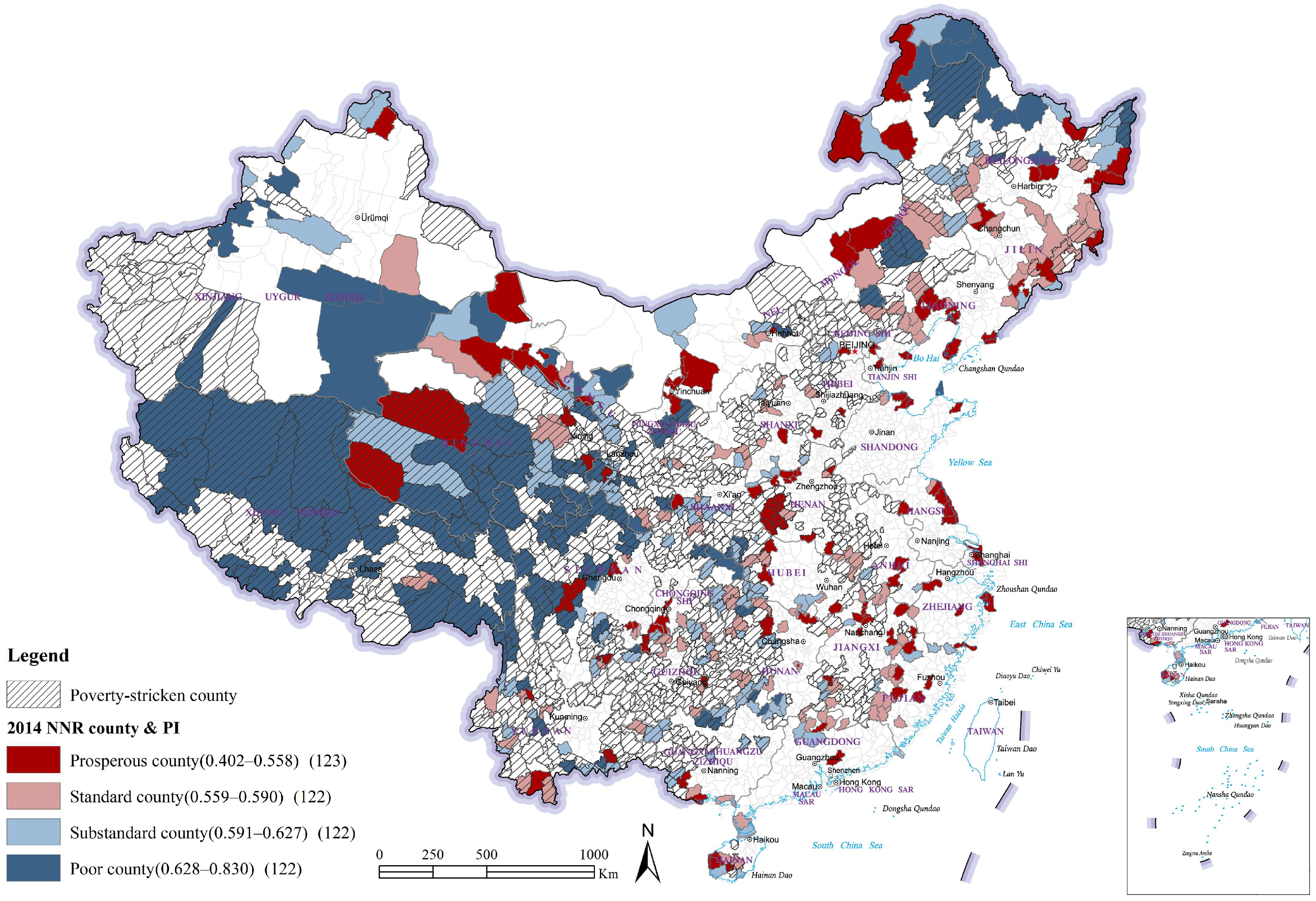
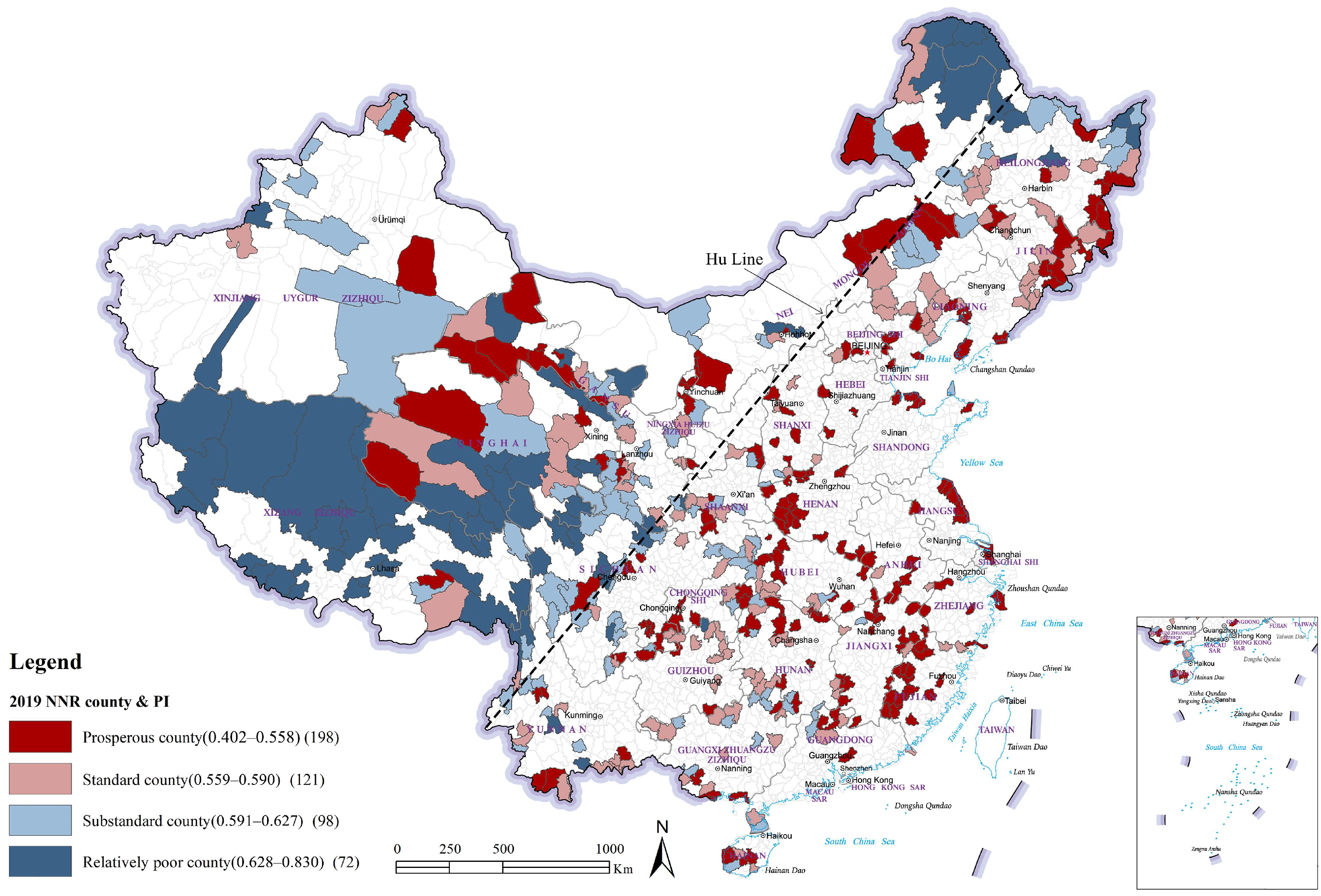
3.1.1. Spatial Distribution of Relative Poverty

Using Equations (1)–(5), the study calculated the PI for each subsystem (natural environment, society, and economy). After determining the environmental, social, and economic poverty indexes, we obtained a PI that characterizes the level of comprehensive regional poverty. To analyze the specific distribution of the relative levels of poverty in each county, the division method of relative poverty population was used as a reference. According to the PI for 2014, the counties were grouped into four equal categories, namely, relatively poor county (0.628 < PI ≤ 0.830), relatively substandard county (0.591 < PI ≤ 0.627), standard county (0.559 < PI ≤ 0.590), and prosperous county (0.402 ≤ PI ≤ 0.558). Figure 2 and Figure 3 illustrate the distribution map of the PI status of the PA counties for 2014 and 2019.
To verify the accuracy of relative poverty evaluation at the county level in the nature reserve area, we compared the evaluation results for 2014 with the list of national poor counties. The results demonstrated that 70.3% of the national poor counties affected by PA are identified as relatively poor and substandard counties. Given that the evaluation of the standard for national poverty counties focuses on the economic dimension, the consideration of social and natural capital factors is lacking, leading to the inconsistency of a small number of results. In summary, the evaluation results of the PI are generally consistent with the list of national poor counties.
According to the results of the PI evaluation for 2019, the relatively poor area of the nature reserves are mainly concentrated in the northwest provinces along the Hu Line (the “Hu Line” has been regarded as one of the greatest geographical discoveries in China because it reveals the significant spatial relationship between human activity and the natural environment [28]), which is highly consistent with key national functioning ecological areas. In 2019, the number of relatively poor counties decreased from 122 to 72, and the number of advantageous counties expanded from 123 to 198 compared with those in 2014. Thus, the overall development has greatly improved.

3.1.2. Evolutionary Characteristics of PI Changes

The study evaluated the change rate of poverty alleviation in PA-affected counties in a graded manner using Equation (6). According to the equal interval algorithm, change rates of 0–10.0% (relatively low), 10.1–20.0% (relatively medium), and 20.1–100% (relatively fast) were used as reference dividers to classify the degree values of the multidimensional poverty change of PA-affected counties into six types, namely, (1) fast-paced improvement zones, (2) mid-range improvement zones, (3) slow improvement zones, (4) slow deterioration zones, (5) mid-range deterioration zones, and (6) rapid deterioration zones. Figure 4 provides the distribution of the change rates.
The study found significant differences in the overall spatial distribution of poverty change. The change rate type of the PI was dominated by relatively slow improvement zones (415), which accounted for 84.87% of the total, and were widely distributed in various regions across China. This was followed by relatively slow deterioration zones (51), which accounted for 10.43% of the total and were mainly distributed among Inner Mongolia, Qinghai, Gansu, and Northeast China. In addition, several counties and districts have changed rapidly in China. Among them, relatively fast pace improvement zones included Pudong New Area of Shanghai and Maojian District of Hubei Province. Based on their advantageous edge, the economic and social developments are the main driving forces of progress. Relatively mid-range deterioration zones were located in Inner Mongolia, where the social dimension is the main cause of their deterioration.
From the perspective of the change rate of the economic dimension, the difference in change rate is small and the degree of spatial aggregation is apparent. The central and southern regions are capable of alleviating poverty, and the majority of them demonstrated slow-speed and medium-speed improvement. Economic development in the west and northeast regions was slow and even exhibited a backward trend; this may be the outcome of eradicating weak economic poverty, which hinders poverty alleviation.
From the perspective of the change rate of the social dimension, the change rate varied greatly and was scattered throughout the country. Although the entire county of the protected area was dominated by slow improvement, the percentage of the overall deterioration reached approximately 23%, out of which deterioration was the most prominent in the north and west regions. The impact of regional social development on the capacity for poverty alleviation was relatively scattered.
From the perspective of the development of the eradication of environmental poverty as a whole, the spatial aggregation trend of the change in the ability to utilize and improve natural resources to alleviate poverty is significant. Among the three dimensions, the optimization rate of the environmental dimension was the slowest, whereas the number of deteriorating counties and districts was the largest, which accounted for 28.8%. The change in natural resources is considered related to population growth and the change in vegetation quality, which indicates that the deprivation of natural resources leads to little result in enhancement.

3.1.3. Spatial Autocorrelation Analysis—Aggregation Characteristics of Spatial Distribution of Poverty

Using ArcGIS to calculate the Global Moran’s I index and the standardized Z-statistics of the multidimensional comprehensive level of poverty of counties and districts in 2014 and 2019 (Table 2), this illustrates a high spatial aggregation effect in the spatial distribution of the multidimensional relative poverty in counties and districts in the reserve. According to the data on the multidimensional PI for 2019, the number of significant spatial aggregation types is 232, which indicates a decrease of six aggregation types compared with the data for 2014. From 2014 to 2019, the environment-caused, economic-eliminating, and social-caused PIs displayed high spatial aggregation effects. Compared with 2014, however, the aggregation of environment- and social-caused PIs was weakened, whereas the economic-eliminating PI remained relatively stable. Among the three dimensions, the aggregation level of the environment-caused PI was higher, which indicates that the current regional poverty situation is greatly constrained by the natural environment. In other words, the regional development has failed to break through this inherent natural constraint such that the relative poverty situation continues.
Combined with the global autocorrelation scatter and local autocorrelation Lisa cluster diagrams, the significance level was set at 0.05. Further analysis of the correlation degree of the PI between relatively poor counties and similar surrounding counties was conducted to obtain the spatial distribution characteristics of the multidimensional comprehensive level of poverty in poor counties.
According to the relation between the statistical value of the local Moran’s I and values of its surrounding areas, the local aggregation characteristics were grouped into four types (Figure 5), namely, high–high aggregation (HH), high–low aggregation set (HL), low–high aggregation (LH), and low–low aggregation sets (LL).
HH type indicates that the degree of poverty in the region is relatively high, and the spatial difference between them is small, indicating a significant spatial positive correlation; 2019 HH-type regions are mainly distributed in the western region and are concentrated in Tibet, Qinghai, northwest Sichuan, southwest Gansu, and the northeast border. These regions are evidently relatively poor as a whole. Therefore, follow-up development policies need to further increase the inclined investment in HH-type agglomeration areas to promote an overall balanced development.
LL type indicates that the poverty level of the region and surrounding adjacent areas is relatively light, and the spatial difference between them is small, indicating a significant spatial positive correlation. A total of 117 counties and districts belong to the LL type, which are mainly distributed in the east of China.
HL type indicates that the comprehensive level of poverty of the region is high, whereas the level of poverty of adjacent areas is low. The multidimensional poverty space of the two is heterogeneous. In 2019, they were sporadically and mainly distributed in relatively poor or standard counties, such as Qingyuan County in Zhejiang Province and Nan’ao County in Guangdong Province. Therefore, strengthening regional interaction and promoting common prosperity are necessary aspects.
LH type indicates that areas with low levels of poverty are surrounded by other areas with high levels of poverty. The two areas exhibit huge spatial differences and are generally distributed in the western region. The majority are relatively advantageous counties, such as Kangding County of Ganzi in Tibetan Autonomous Prefecture in Sichuan Province and Motuo County in Tibet. Both receive strong support from policies such as the “Development of Western Region” and “Targeted Poverty Alleviation.” Thus, considerable progress has been achieved in the development of basic infrastructure construction and environmental conservation. However, the radial impact of such areas on their surrounding regions needs to be strengthened further.

3.2. Multidimensional Composite Poverty Dominant Factor Analysis

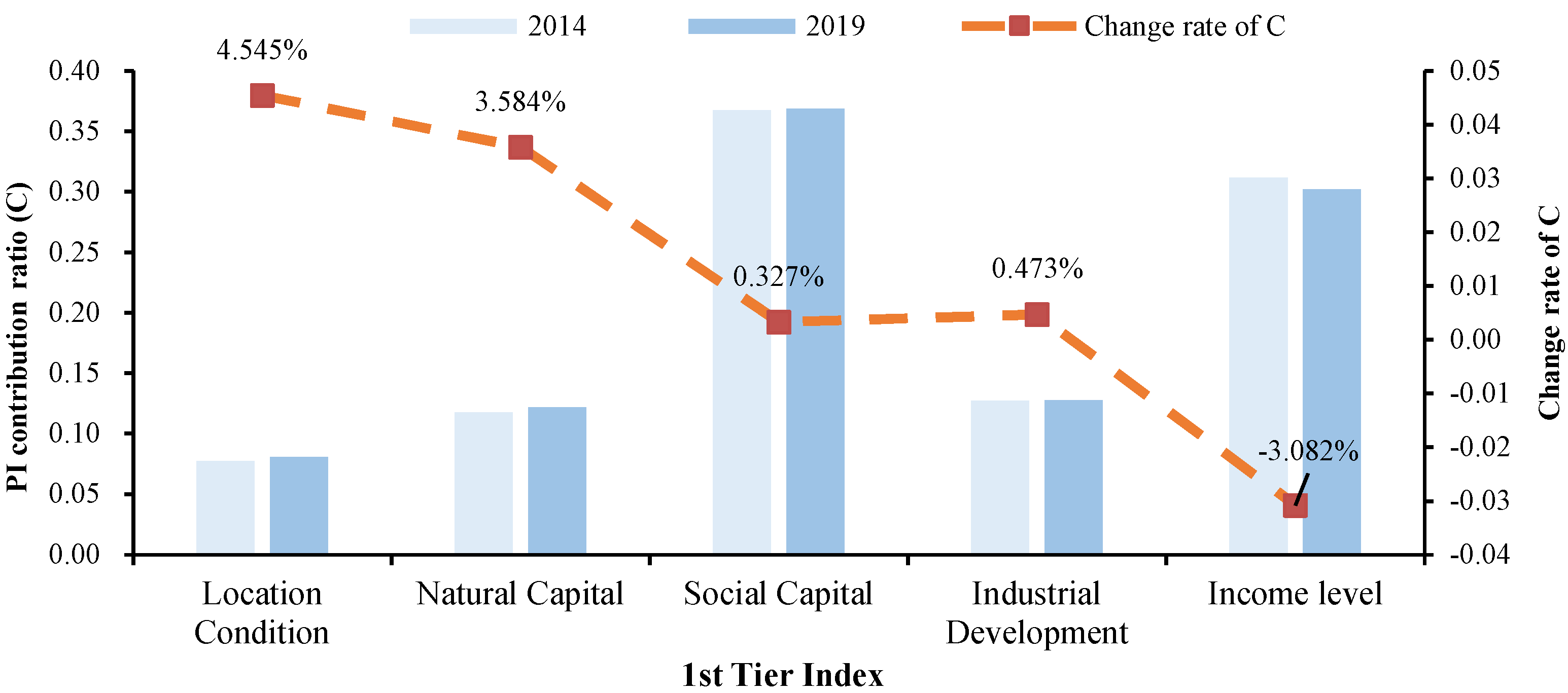
3.2.1. Multidimensional Integrated Poverty Contribution and Its Change

Using Equation (7), we calculated the PI contribution ratio C for each dimension to identify the driving factors of the evolution of the PI. Thus, the accuracy of poverty targeting as well as the targeting of poverty reduction measures can be enhanced. Figure 6 illustrates the following: (1) the environment system has a lower contribution to poverty but the largest increase in the rate of change of the contribution, which indicates that these objective natural environmental conditions exert a greater impact on the change of the PI. (2) The level of economic development has a high contribution to poverty and decreased in 2019. This change is mainly reliant on the relative increase in income levels, whereas the industrial structure needs further enhancement. (3) The contribution rate of the social dimension lies in the middle without much change. In other words, the lack of improvement in location conditions, natural capital, industrial development, and social capital are the main factors that lead to the increase in the contribution rate C of the multidimensional comprehensive poverty. Among them, location conditions and natural capital are the most significant. For the relatively poor counties that are PA-affected, stabilizing the quality of poverty eradication should continue to improve the level of economic development and promote the social guarantee system. In addition, it should strengthen the protection of ecological resources and improve environmental quality to maximize the joint force of the three dimensions in accelerating comprehensive and sustainable development.

3.2.2. Cluster Analysis
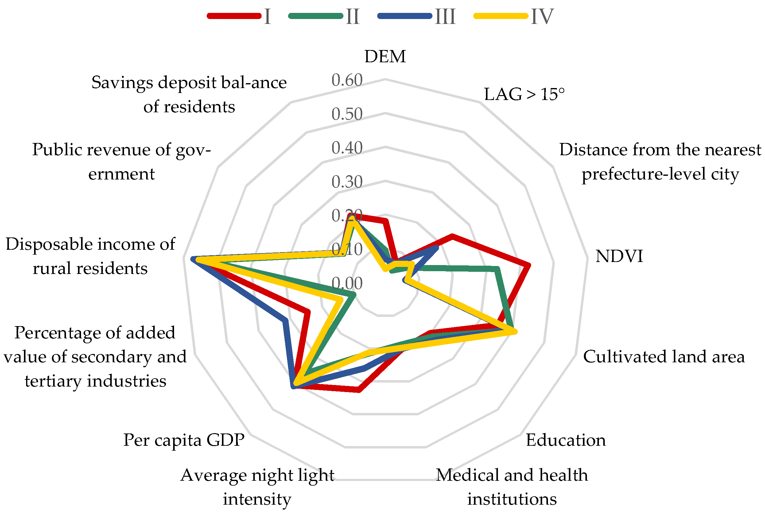
(1)
Cluster analysis of 489 counties
The prerequisite for making policy recommendations to facilitate poverty reduction through multidimensional poverty measures is the analysis of poverty-driving mechanisms, which may vary across PA-affected counties with similar PI. The cluster analysis is based on the similarity and difference of the PI of PA-affected counties combined with distance statistics. The scientific and comprehensive level-by-level consolidation of PA-affected counties can ensure the efficient categorization of similar poverty-driving mechanisms and achieve the effect of dimensionality reduction simultaneously. Pudong New Area was extracted separately prior to the cluster analysis owing to its extremely low poverty level. Using 13 dimensions as the independent variables, the K-means cluster analysis was conducted using SPSS 23 on the subdimensional PI values of 488 counties for 2019.
The clustering results and F-test (Table 3) illustrate that the unweighted regression has nonsignificant clustering results in certain dimensions. Nevertheless, the weighted regression demonstrated significant result in all dimensions; hence, subsequent analysis was conducted based on the results of the weighted regression. Through the cluster analysis, all counties were aggregated into four categories (Table 4 and Figure 7). By referring to the comparison of the poverty contribution ratio C for each indicator of the four categories (Figure 8), the study explored the poverty-driving mechanisms of each county from multiple perspectives.
Under Category I (red), NNR counties are regions constrained by natural conditions with high PI. High PI and high poverty contribution rate of natural dimension were characterized by high poverty coefficients of the geographical (DEM, slope) dimension. The study identified 31 counties under this category, which comprise three relatively substandard counties and 26 relatively poor counties and accounts for 9.68% and 83.9% respectively. These counties tend to exhibit a slow rate of improvement, and are mainly located in western China.
Counties under Category II (green) had a relatively lower PI but its dimension of natural resource was weak. The only problem comes from the environment system. Moreover, the counties were mainly distributed among the suburbs of plain land cities. Within the 62 counties, 18 were relatively substandard counties and 10 were relatively poor counties, which accounted for 29.0% and 16.1%, respectively. The relatively low rate of deterioration in these counties accounted for a relatively large proportion of counties and districts, which indicates the slow industrial development and presence of constant ecological deterioration.
Counties under Category III (blue) exhibited a slightly higher PI as well as a higher PI contribution in the economic dimensions, and were classified to be relatively lagging economies. These counties are mainly located in the suburbs of large cities. Within the 89 counties, 30 were relatively substandard counties were 32 are relatively poor counties, which accounted for 33.7% and 36.0%, respectively. Considering that this may be influenced by the siphon effect of big cities [25], leading to the loss of self-development factors, most of these counties have a relatively low rate of improvement.
Under Category IV (orange), counties were basically low in PI, which indicates that the majority are not relatively poor counties. They had better development in three dimensions, namely, economic production, social resources, and environmental resources, and had more counties and districts with optimized industrial policies. This category holds the largest number of counties at 306, including 51 relatively substandard counties and eight relatively poor counties and accounted for 16.7% and 0.03%, respectively. Most of these counties exhibited relatively low rates of improvement, whereas a few had medium to high rates of improvement. However, they continue to require effort in promoting green development under the influence of the ecological environment protection.
(2)
Analysis of poverty-aggravated counties among relatively poor counties
In order to further define the main causal factors of poverty in continuously deteriorating relatively poor counties, the study sieved out these counties from 2014 and 2019 according to the PI of the deprivation index and classified them into two groups, namely, poverty-aggravated and poverty-reduced, based on their rate of change in PI. According to the results of the significance test, 22 poverty-aggravated counties were divided into three categories (Figure 9, Table 5).
The dimensionality clustering result showed that counties from all three categories were lacking in terms of income; amongst them, Categories I and II were notably limited in the social dimension. Combined with the analysis results of the rate of change C, spatial correlation, and global clustering, etc., the results are as follows.
Compared with counties from other categories, the NTL index of Category-1 counties had a more apparent impact on PI. These counties are mainly located in southwest China and do not comprise LH counties. The overall social and economic development level of these poverty-stricken counties are relatively weak as their active populations are low. For counties with limited production capability, their relief strategies include expanding industrial functions of villages and towns while promoting county infrastructure development, encouraging moderate scale agricultural production, boosting comparative agricultural efficiency, enhancing rural construction, promoting non-agricultural industries, and optimizing the organizational network of multiple social subjects.
The PI was relatively high for Category-2 counties. Compared with other clusters, the level of education in the social dimension was the main factor causing poverty under this category. That is, counties within this cluster should emphasize the conservation of natural resources to alleviate poverty. These counties can adopt relief strategies such as improving school conditions in township schools, and improving the accessibility of educational resources by improving school layout and education guarantee mechanisms according to the actual situation of specific towns and villages.
The PI of Category-3 counties was relatively high. Apart from lofty contribution from the social dimension, distance from prefecture-level cities was also an influential factor in limiting the development of these counties. More HL counties were found under Category III, which indicates that counties in this category were relatively underdeveloped and are potential victims to the “spatial poverty trap”. Therefore, it is possible to form a new urban–rural relationship integrating urban and rural areas by strengthening the county’s overall planning and optimizing infrastructure construction.

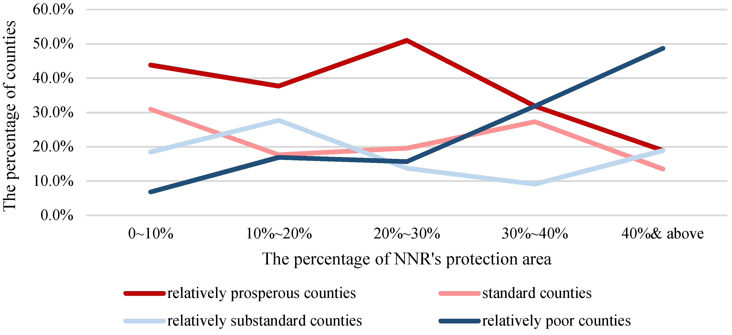
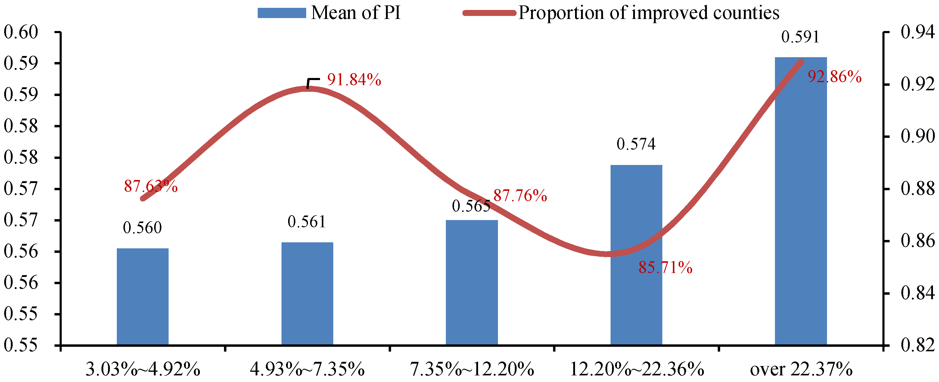
3.3. Do Protection Zones Exacerbate Poverty—Analysis of Correlation Characteristics Based on the Percentage of Protection Area and Degree of Poverty

To verify the correlation between the percentage of PA in the research sample and poverty, the 489 PA and counties were grouped into relatively poor and non-poor counties corresponding to the list of national poor counties up to 2019. Comparing the percentage of PA under the NNR in the two types of counties, the average percentage of PA in relatively poor counties was 23.74%, whereas the average percentage of PA in non-poor counties was 12.73%. This result implies that the portion of PA in poor counties is significantly wider than that in non-poor counties, and a correlation may exist between protection zone and level of poverty.
Subsequently, the 2019 PI results of regions with high and low percentages of PA were compared, which presented an evident positive correlation between the percentage of PA and degree of poverty. According to the evaluation of the PI degree, relatively poor counties are mainly distributed in the northwest provinces along the Hu Line and points to large differences from non-poor counties in terms of per capita GDP, income level, and social conditions (Table 6, Figure 10). Analysis using the Pearson correlation’s coefficient (sample linear correlation coefficient) indicated that the area percentage of NNR has a significant correlation with the PI of corresponding districts and counties (correlation coefficient: 0.281, significance: 0.01).
To observe the dynamic changes between the change rate of the PI and the percentage of PA in counties and regions from 2014 to 2019, the protected counties were classified into five groups, which range from small to large according to the percentage of PA. Each group comprises 97–98 counties. The average values of the PI for each group were subsequently compared with the percentage of poverty-improved counties. Figure 11 illustrates an apparent positive correlation between county poverty and the percentage of PA. However, the counties affected by PA exhibited different degrees of poverty reduction, where counties with more than 22% of PA had the highest poverty improvement rate. Therefore, no evidence exists to prove that the expansion of PA necessarily exacerbates poverty deterioration; moreover, environmental protection does not necessarily come at the expense of regional development.
Combined with the results of the cluster analysis of each group of counties and districts, this study analyzed the effect of various natural resource conditions on the causative factors of poverty under various proportions of reserve areas. The results demonstrated that the number of counties restricted by natural resources increases according to the increase in the proportion of PA. However, the effect of poverty reduction demonstrated in the comprehensive dimension was more apparent owing to the optimization of ecological environment in counties with higher proportions of PA, decreased influence of the economic dimension, and increased influence of the environmental dimension on the contribution rate of the PI.

4. Discussion

Ecology and poverty are closely related, especially in regions affected by PA, where the phenomenon of “rich poverty” frequently occurs. This tendency reflects problems in the economic structure, balanced regional development, and equalization of basic services, which may aggravate the gap between the rich and poor. Thus, identifying the degree and type of relative poverty is a prerequisite to the solution of the aforementioned problem to achieve common prosperity.
Using rich spatial data and socioeconomic statistics, this study examined 489 PA-affected counties as research subjects through the multidimensional integrated poverty metric model for nature reserve counties. In the process, all counties’ multidimensional integrated PI with the change and spatial autocorrelation characteristics were systematically measured and analyzed. Furthermore, K-means clustering and contribution rate were used to quantitatively analyze the driving factors of multi-dimensional comprehensive poverty from 2014 to 2019. Under the influence of increasingly complex causative factors of poverty due to county development, the paper further explored the relationship between the scale of PA and the level of relative poverty.
Our study revealed for the first time the spatial distribution pattern of relative poverty areas affected by NNR in China. Most of the relatively poor counties are located in the western and northeastern regions of China with a spatial aggregation effect. In terms of evolutionary characteristics and drivers, most of the poor counties still have difficulty in overcoming the natural resource constraints, as the environmental and social dimensions lack engagement. These leads to 10.8% of NNR counties showed a trend of aggravating multidimensional poverty. Therefore, future development need more engagement on ecological protection and social progress, especially on the implementation of policies conducive to decoupling development, effectively preventing poverty due to environmental degradation.
In addition, nature conservation and PI are closely related, but the expansion of PA does not necessarily lead to aggravation of poverty. Instead, the establishment of PA may help in the alleviation of multidimensional poverty. Though it differs from our past understanding [29], it adds on to the Chinese empirical case studies for related research in PA’s impact on the impoverishment of communities [21,30]. However, PA may have had other impacts on local people, such as living conditions, equity, and social networks, which were not captured in this paper and would rely on more detailed social surveys in the future.
In sum, it is essential to know that expanding the network of PA not only helps to cope with the loss of biodiversity and environmental degradation, but also helps to enhance the integrated sustainable development. However, many challenges are still in the way of maintaining the efforts of ecological poverty reduction. Based on this, combined with the results of dimensional analysis, we propose the following policy recommendations respectively.
For regions where natural factors cause poverty, considering the relative poverty is mainly caused by the restrictions of PA or limited available natural resources that are not suitable for large-scale development. On the one hand, the supply of ecological compensation policies should be continuously ensured to safeguard the basic rights and interests of communities [31]; on the other hand, the trading mechanism of PA indicators should be actively explored [32], while shifting to an eco-friendly development model.
The relatively lagging economy type of relatively poor counties are mostly influenced by the siphoning effect of surrounding large cities. Facing the loss of rural production factors, such areas have a sole industrial structure and low production efficiency in local industries, which hinders production development. Thus, integrated strategies, such as more intensive use of land, enhancement of regional connection, and inputs on eco-tourism [33] and eco-brand integrated with local PA [34], should be conducted to cultivate new sustainable growth factors to compensate for the shortcomings in development.
For the counties with social poverty, the lack of public services and social vigor are the main cause of poverty. Thus, there is a need to improve the conditions of schools and accessibility to educational resources [35]. Besides, collaboration among government, local communities, and firms is also essential to encouraging a more harmonious society.

5. Conclusions

China bid farewell to “absolute poverty” in 2020. However, PA-affected communities may continue to suffer from “relative poverty” or “multidimensional poverty”, becoming a challenge to stabilizing our efforts of poverty alleviation. Some researchers have shown that PA could have a negative impact on its local communities and can even be a “poverty trap” [36]. In the game of conservation and development, the issue of relative poverty will indirectly influence the construction of PA networks. This study is one of the few to explore the spatial identification of relative poverty in protected areas, and its results suggest the following.
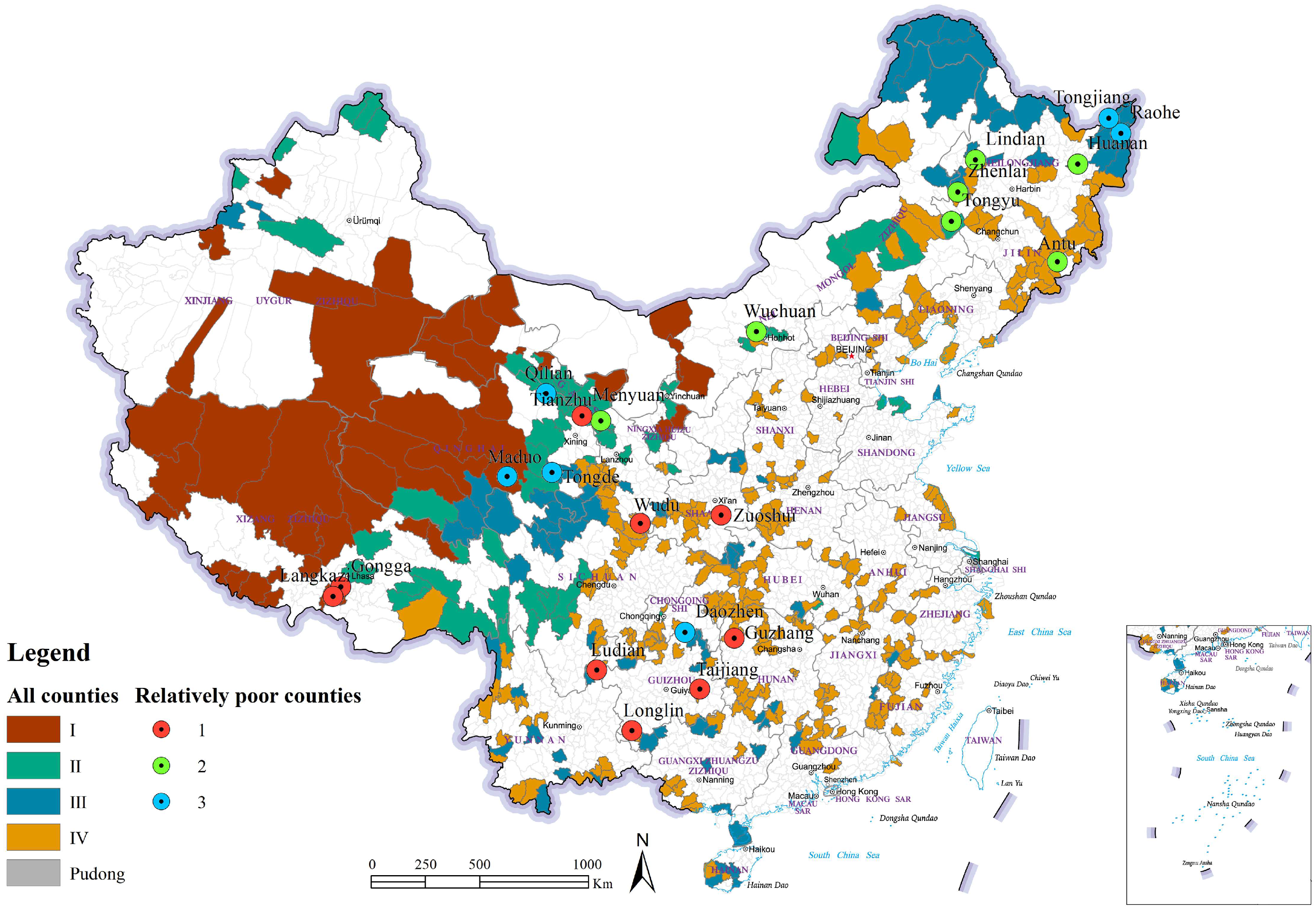
  • There were 72 PA relatively poor counties in 2019, mostly located in the northwestern provinces of China (Figure 3). The poverty situation in the PA-affected counties has generally improved at a relatively slow pace. However, there are still a total of 22 counties with high level of poverty and a trend of aggravating poverty (Figure 7), which are the key areas for securing and stabilizing of poverty alleviation in the future.
  • Referring to the driving factors analysis, the poverty causation mechanisms of all PA counties were grouped under four categories, namely, natural condition constraint type, natural resource disadvantaged type, economic lagging type, and integrated green developing type. Poverty relief should be considered during infrastructure upgrade, ecological improvement, industrial and production optimization, and sustainable green development. As for relatively poor counties, the main cause of poverty originates from the social dimension, where the lack of socioeconomic vitality and education is the primary driving factor.
  • Attested to by correlation, a strong positive interrelationship was observed between the protected portion of PA counties and multidimensional integrated poverty PI. This scenario may be the result of the selective zoning of PA in regions with high biodiversity conservation values and low development potential. However, no direct evidence exists to prove that the expansion of PA necessarily exacerbates poverty deterioration; instead, counties with 22% or more PA showed the highest improvement rates. It is comforting to know that the expansion of PA in China holds no causal relationship to the aggravation of poverty, and in certain cases, it can even contribute to poverty reduction.
Finally, this study may have its limitations. Certain omissions of indicators in the index system may have occurred owing to difficulties in obtaining official data at the county scale. Thus, exploring the influence of PA in developing countries on socioeconomic development, including sustainable livelihood, health, and community co-management, would be meaningful. The current data are insufficient to justify or discuss these issues, indicating that a longer period of monitoring work is required to comprehensively track the impact of PA on the environment and socioeconomic development.

Author Contributions

Conceptualization, methodology, and formal analysis, X.H.; data curation, software, validation, visualization and writing—original draft preparation, X.H., A.L. and J.L.; resources, Y.Z., X.H. and A.L.; writing—review and editing, X.H. and Y.Z.; supervision and funding acquisition, Y.Z. All authors have read and agreed to the published version of the manuscript.

Funding

This research was funded by The National Social Science Fund of China under a project entitled “Research on Establishing a Protected Area System in China with National Parks as the Mainstay” (Project No. 18BGL178).

Institutional Review Board Statement

Not applicable.

Informed Consent Statement

Not applicable.

Data Availability Statement

The data that support our research findings are available from the corresponding author on request.

Conflicts of Interest

The authors declare no conflict of interest.

References

  1. Adams, W.M.; Aveling, R.; Brockington, D.; Dickson, B.; Elliott, J.; Hutton, J.; Roe, D.; Vira, B.; Wolmer, W. Biodiversity conservation and the eradication of poverty. Science 2004, 306, 1146–1149. [Google Scholar] [CrossRef] [PubMed] [Green Version]
  2. Gray, L.C.; William, G.M. A geographical perspective on poverty–environment interactions. Geogr. J. 2005, 171, 9–23. Available online: https://www.jstor.org/stable/3451384 (accessed on 5 June 2022). [CrossRef]
  3. Jehan, S.; Umana, A. The environment-poverty nexus. Dev. Policy J. 2003, 3, 53–70. [Google Scholar]
  4. Awad, A.; Warsame, M.H. The poverty-environment nexus in developing countries: Evidence from heterogeneous panel causality methods, robust to cross-sectional dependence. J. Clean. Prod. 2022, 331, 129839. [Google Scholar] [CrossRef]
  5. Yang, R.; Cao, Y.; Hou, S.; Peng, Q.; Wang, X.; Wang, F.; Tseng, T.-H.; Yu, L.; Carver, S.; Convery, I.; et al. Cost-effective priorities for the expansion of global terrestrial protected areas: Setting post-2020 global and national targets. Sci. Adv. 2020, 6, eabc3436. [Google Scholar] [CrossRef] [PubMed]
  6. Cernea, M.M.; Schmidt-Soltau, K. Poverty risks and national parks: Policy issues in conservation and resettlement. World Dev. 2006, 34, 1808–1830. [Google Scholar] [CrossRef]
  7. Mammides, C. Evidence from eleven countries in four continents suggests that protected areas are not associated with higher poverty rates. Biol. Conserv. 2020, 241, 108353. [Google Scholar] [CrossRef]
  8. Chang, J. Achievements of China’s Eco-environmental Protection in 2018 and Challenges in 2019 Under Green Development Perspective. Environ. Prot. 2019, 47, 37–40. (In Chinese) [Google Scholar] [CrossRef]
  9. Wang, H.Y.; Qian, L.Y.; Chen, Y.F. Multidimensional and comprehensive poverty measurement of poverty-stricken counties from the perspective of ecological poverty. Chin. J. Appl. Ecol. 2017, 28, 2677–2686. (In Chinese) [Google Scholar] [CrossRef]
  10. Liu, Y.H.; Xu, Y. A geographic identification of multidimensional poverty in rural China under the framework of sustainable livelihoods analysis. Appl. Geogr. 2016, 73, 62–76. [Google Scholar] [CrossRef]
  11. Liu, Y.H.; Xu, Y. Geographical identification and classification of multi-dimensional poverty in rural China. Acta Geogr. Sin. 2015, 70, 993–1007. (In Chinese) [Google Scholar]
  12. Liu, X.M.; Han, L.Z.; Zheng, J.H. Temporal-Spatial Characteristics and the Driving Mechanism of Multidimensional Comprehensive Poverty Degree in Poverty-Stricken Counties: A Case Study of Poor Counties in Deep Poverty-Stricken Areas of Southern Xinjiang. Econ. Geogr. 2019, 39, 165–174. (In Chinese) [Google Scholar] [CrossRef]
  13. Wang, W.; Yu, C.; Zeng, X.; Li, C. Evolution characteristics and driving factors of county poverty degree in China’s southeast coastal areas: A case study of Fujian Province. Prog. Geogr. 2020, 39, 1860–1873. (In Chinese) [Google Scholar] [CrossRef]
  14. Xu, L.D.; Deng, X.Z.; Jiang, Q.O. Identification and poverty alleviation pathways of multidimensional poverty and relative poverty at county level in China. Acta Geogr. Sin. 2021, 76, 1455–1470. (In Chinese) [Google Scholar]
  15. Alkire, S.; Foster, J. Understandings and misunderstandings of multidimensional poverty measurement. J. Econ. Inequal. 2011, 9, 289–314. [Google Scholar] [CrossRef] [Green Version]
  16. Sen, A. A sociological approach to the measurement of poverty: A reply to Professor Peter Townsend. Oxf. Econ. Pap. 1985, 37, 669–676. Available online: http://www.jstor.org/stable/2663049 (accessed on 4 July 2022). [CrossRef]
  17. Pan, J.H.; Hu, Y.X. Spatial Identification of Multidimensional Poverty in China Based on Nighttime Light Remote Sensing Data. Econ. Geogr. 2016, 36, 124–131. (In Chinese) [Google Scholar] [CrossRef]
  18. Chen, Q.; Lu, S.; Xiong, K.; Zhao, R. Coupling analysis on ecological environment fragility and poverty in South China Karst. Environ. Res. 2021, 201, 111650. [Google Scholar] [CrossRef] [PubMed]
  19. Jiang, A.Y.; Feng, Y.J. The County’s Poverty Assessment in Concentrated Destitute Areas of Liupanshan–on Improved HDI. J. Shijiazhuang Univ. Econ. 2015, 38, 1–6. (In Chinese) [Google Scholar] [CrossRef]
  20. Alkire, S.; Foster, J. Counting and multidimensional poverty measurement. J. Public Econ. 2011, 95, 476–487. [Google Scholar] [CrossRef] [Green Version]
  21. Canavire-Bacarreza, G.; Hanauer, M.M. Estimating the impacts of Bolivia’s protected areas on poverty. World Dev. 2013, 41, 265–285. [Google Scholar] [CrossRef] [Green Version]
  22. Cheng, X.; Shuai, C.; Liu, J.; Wang, J.; Liu, Y.; Li, W.; Shuai, J. Topic modelling of ecology, environment and poverty nexus: An integrated framework. Agric. Ecosyst. Environ. 2018, 267, 1–14. [Google Scholar] [CrossRef]
  23. Zhao, Z.C.; Zhong, L.; Yang, R. Discussion on the nature reserves as foundation of protected areas in the new era of ecological civilization. Chin. Landsc. Archit. 2020, 36, 6–13. [Google Scholar] [CrossRef]
  24. Pan, J.H.; Feng, Y.Y. Spatial distribution of extreme poverty and mechanism of poverty differentiation in rural China based on spatial scan statistics and geographical detector. Acta Geogr. Sin. 2020, 75, 769–788. (In Chinese) [Google Scholar] [CrossRef]
  25. Xu, Z.; Sun, T. The Siphon effects of transportation infrastructure on internal migration: Evidence from China’s HSR network. Appl. Econ. Lett. 2021, 28, 1066–1070. [Google Scholar] [CrossRef]
  26. Wang, Y.; Chen, Y. Using VPI to Measure Poverty-Stricken Villages in China. Soc. Indic. Res. 2017, 133, 833–857. [Google Scholar] [CrossRef]
  27. Bird, K.; Mckay, A.; Shinyekwa, I. Isolation and Poverty: The Relationship between Spatially Differentiated Access to Goods and Services and Poverty; Overseas Development Institute (ODI): London, UK, 2011; p. 322. [Google Scholar]
  28. Qi, W.; Liu, S.; Zhao, M.; Liu, Z. China’s different spatial patterns of population growth based on the “Hu Line”. J. Geogr. Sci. 2016, 26, 1611–1625. [Google Scholar] [CrossRef]
  29. Meijaard, E.; Sheil, D. Cuddly animals don’t persuade poor people to back conservation. Nature 2008, 454, 159. [Google Scholar] [CrossRef]
  30. Andam, K.S.; Ferraro, P.J.; Sims, K.R.E.; Healy, A.; Holland, M.B. Protected areas reduced poverty in Costa Rica and Thailand. Proc. Natl. Acad. Sci. USA 2010, 107, 9996–10001. [Google Scholar] [CrossRef] [PubMed] [Green Version]
  31. Ola, O.; Menapace, L.; Benjamin, E.; Lang, H. Determinants of the environmental conservation and poverty alleviation objectives of Payments for Ecosystem Services (PES) programs. Ecosyst. Serv. 2019, 35, 52–66. [Google Scholar] [CrossRef]
  32. Yang, R.; Zhong, L.; Zhao, Z.C. Index trading mechanism of nature reserves based on consumer end: Value realization of ecological products. J. Ecol. 2020, 40, 6687–6693. (In Chinese) [Google Scholar]
  33. Agrawal, A. Matching and mechanisms in protected area and poverty alleviation research. Proc. Natl. Acad. Sci. USA 2014, 111, 3909–3910. [Google Scholar] [CrossRef] [PubMed] [Green Version]
  34. Chi, N. Understanding the effects of eco-label, eco-brand, and social media on green consumption intention in ecotourism destinations. J. Clean. Prod. 2021, 321, 128995. [Google Scholar] [CrossRef]
  35. Oldekop, J.A.; Holmes, G.; Harris, W.E.; Evans, K.L. A global assessment of the social and conservation outcomes of protected areas. Conserv. Biol. 2016, 30, 133–141. [Google Scholar] [CrossRef] [PubMed] [Green Version]
  36. Xu, W.G.; Qin, W.H.; Liu, X.M. Status quo of distribution of human activities in the National Nature Reserves. J. Ecol. Rural Environ. 2015, 31, 802–807. (In Chinese) [Google Scholar]
Figure 1. Distribution of research samples.
Land 11 01048 g001
Figure 2. Spatial distribution patterns of four categories of counties affected by PA in 2014.
Land 11 01048 g002
Figure 3. Spatial distribution patterns of four categories of counties affected by PA in 2019.
Land 11 01048 g003
Figure 4. Spatial pattern of the PI change rate.
Land 11 01048 g004
Figure 5. Aggregation map of the local spatial association of multidimensional relatively poor counties in 2019.
Land 11 01048 g005
Figure 6. Analysis of the rate of change of poverty contribution according to the direction for 2014 and 2019.
Land 11 01048 g006
Figure 7. Dimensionality clustering.
Land 11 01048 g007
Figure 8. Comparison of the intensity of the poverty contribution ratio.
Land 11 01048 g008
Figure 9. Clustering result of poverty-aggravated counties.
Land 11 01048 g009
Figure 10. Percentage of protected area and number of counties and districts in 2019.
Land 11 01048 g010
Figure 11. Percentage of the PI in groups of PA counties.
Land 11 01048 g011
Table 1. Framework of the comprehensive poverty measurement.
SystemWeight1st Tier
Index
Weight   ( ω ) 2nd Tier IndexUnitDirectionAHP
(u)
EVM
(v)
Weight   ( λ ) Indicator
Description
Natural Environment (N)1Nature
Resource
0.4NDVI average value (NDVI)\-0.3490.9410.586Reflect the surface
vegetation coverage
per capita cultivated land area (CLA)Hectare-0.6510.0590.414Reflect the supporting capacity of cultivated land
resources for poverty
alleviation
Geographical Conditions0.6elevation (DEM)m+0.1710.3640.229The higher the elevation is, the worse the living conditions are
percentage of land area with gradient >15° (LAG > 15°)%+0.1850.3530.235Reflect the percentage of difficult-to-use land
Distance from the nearest prefecture-level city (DC)km+0.6440.2830.536Reflect the traffic
location; the farther the distance is, the higher the cost of
industrial
development is
Economy(E)1Industrial Development0.4per capita GDP10k yuan-0.5460.1470.426Reflect the level of
regional
social and economic
development
percentage of added value of secondary and tertiary industries (PSTI)%-0.4540.8530.574Driving force of sustainable poverty
alleviation
Income Level0.6Per capita public
revenue of government (PRG)
yuan-0.1480.1900.156Government revenue
capacity
Per capita disposable income of rural
residents (DIRR)
yuan-0.6700.3740.611Reflect the
income level of rural
community
Per capita savings
deposit balance of residents within
entire county (SDBR)
yuan-0.1820.4350.233Reflect the overall
income level of the
country
Society(S)1Social Capital1Number of students per 10k people
(Education)
\-0.3580.3410.353Popularization of
education
Number of beds in medical and health institutions per 10k people (MHI)\-0.2480.1980.233Reflect the level of
medical
security
Average night light intensity (ANLI)\-0.3940.4610.414Reflect
human
activities and urban
built-up area
Table 2. Spatial autocorrelation test of the Poverty Index of PA counties.
IndicatorsMoran’s IZ
2014201920142019
PI0.3040.29716.21915.850
N0.3950.38921.02820.763
E0.2640.26914.10214.550
S0.1210.0996.5245.341
Table 3. F-test of the PI.
IndexF (Unweighted Regression)F (Weighted Regression)
Elevation (DEM)123.73 ***143.83 ***
Percentage of land area with gradient >15°6.29 ***39.81 ***
Distance from the nearest prefecture-level city8.51 ***98.34 ***
NDVI average value992.32 ***481.31 ***
Per capita cultivated land area21.04 ***25.83 ***
Number of students per 10,000 people6.38 ***5.39 ***
Number of beds in medical and health institutions per 10,000 people4.96 ***6.98 ***
Average night light intensity10.79 ***84.29 ***
Per capita GDP45.14 ***46.77 ***
Percentage of added value of secondary and tertiary industries0.546.90 ***
Per capita disposable income of rural residents47.67 ***26.28 ***
Per capita public revenue217.59 ***26.95 ***
Per capita savings deposit balance of residents26.22 ***23.78 ***
Note: *** p < 0.01.
Table 4. Cluster centers and mean square.
IndexCluster CenterMs
IIIIIIIV
Elevation (DEM)0.070.040.200.070.29
Percentage of land area with gradient >15°0.100.050.090.020.11
Distance from the nearest prefecture-level city0.200.070.190.100.53
NDVI average value0.050.070.350.382.18
Per capita cultivated land area0.400.410.370.390.02
Number of students per 10,000 people0.230.240.210.230.01
Number of beds in medical and health institutions per 10,000 people0.200.190.200.180.01
Average night light intensity0.250.210.350.200.25
Per capita GDP0.510.490.510.420.09
Percentage of added value of secondary and tertiary industries0.340.330.340.330.01
Per capita disposable income of rural residents0.130.130.140.120.00
Per capita public revenue0.600.600.600.570.01
Per capita savings deposit balance of residents0.200.200.220.180.01
Table 5. Representing counties from different clusters.
ClusterCounties
1Guzhang, Longlin, Taijiang, Ludian, Gongga, Langkazi, Zuoshui, Wudu, and Menyuan
2Wuchuan, Zhenlai, Tongyu, Antu, Lindian, Huanan, and Tianzhu
3Raohe, Tongjiang, Daozhen, Qilian, Tongde, and Maduo
Table 6. Comparison between relatively poor and non-poor counties in NNR.
TypePercentage of Protected Area%GDP per
Capita/Yuan
Per Capita
Disposable Income of Rural
Residents/Yuan
Number of
Students in School per 10,000 People
Number of Beds in Medical and Health Institutions per 10,000 People
Relatively poor counties23.74%23,538.019574128358
Non-poor counties12.73%53,685.9012,0311116176
Publisher’s Note: MDPI stays neutral with regard to jurisdictional claims in published maps and institutional affiliations.

