
Digital Mapping of Land Cover Changes Using the Fusion of SAR and MSI Satellite Data


Abstract
:1. Introduction
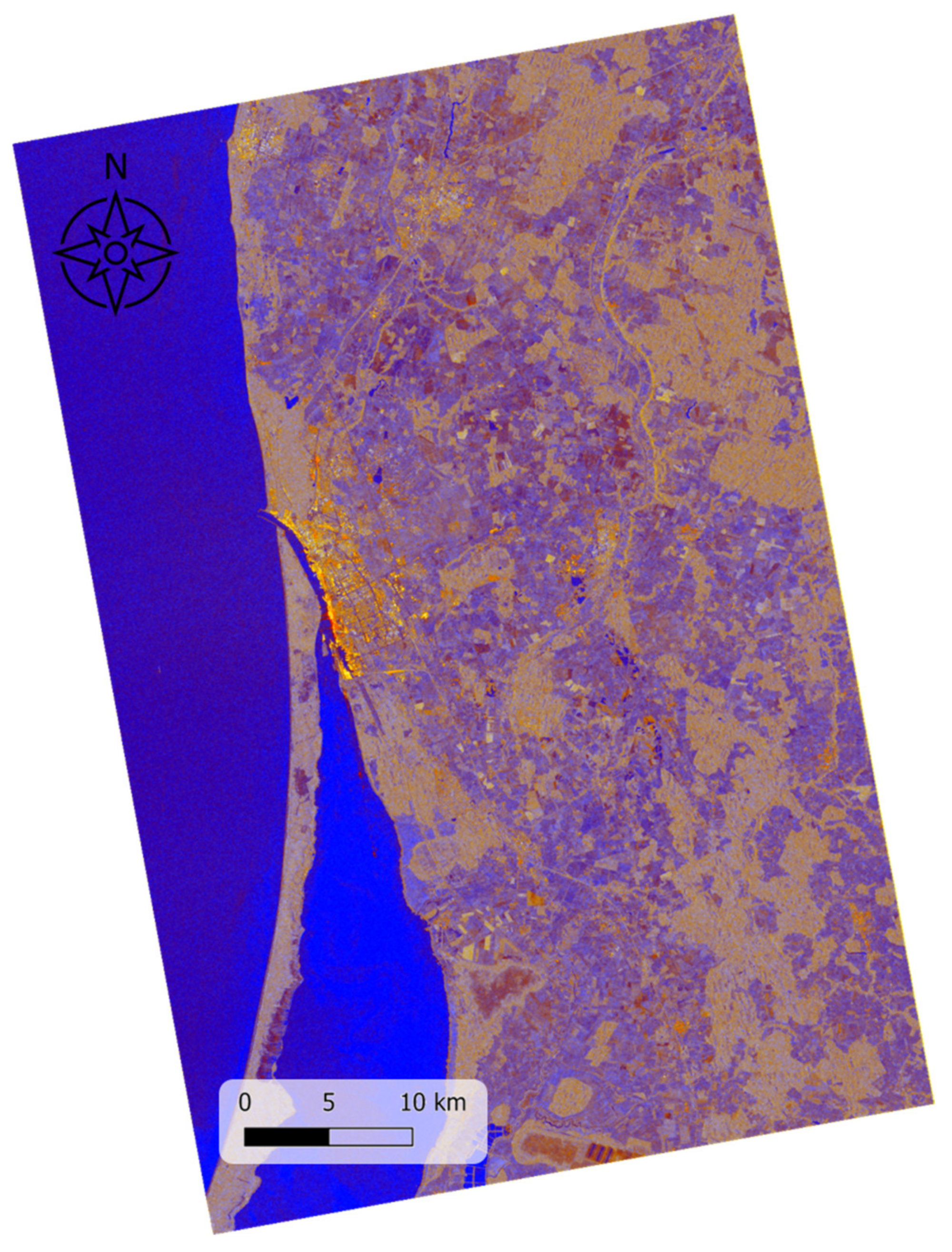
2. Study Area
3. Materials and Methods
3.1. Data Acquisition and Pre-Processing
3.1.1. Pre-Processing of Sentinel-1 SAR Satellite Data
3.1.2. Pre-Processing of Sentinel-2 MSI Satellite Data
3.2. Segmentation and Land Cover Classification
- The coherence of two SAR images;
- The method when SAR and MSI images are segmented separately and the results of segmentation are fused;
- The method when SAR and MSI data are fused before land cover segmentation;
- The upgraded method of SAR and MSI data fusion by adding additional formulas and index images.
3.2.1. The Coherence of Two SAR Images
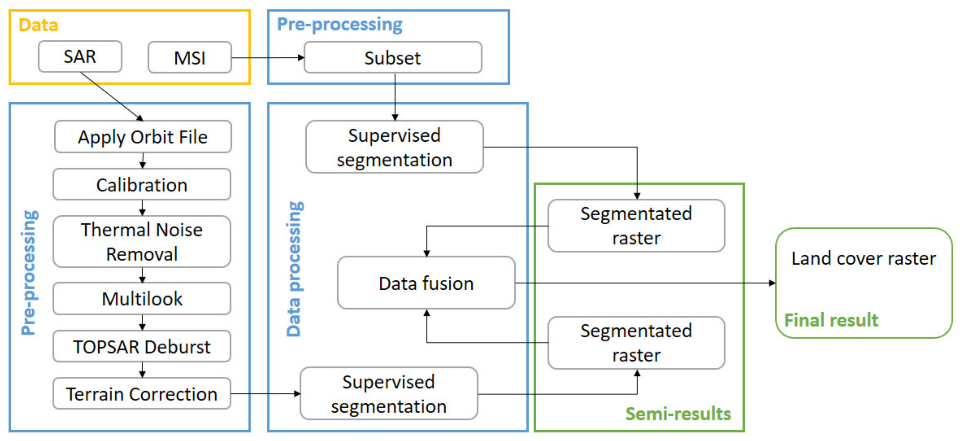
3.2.2. Separate SAR and MSI Segmentation Method
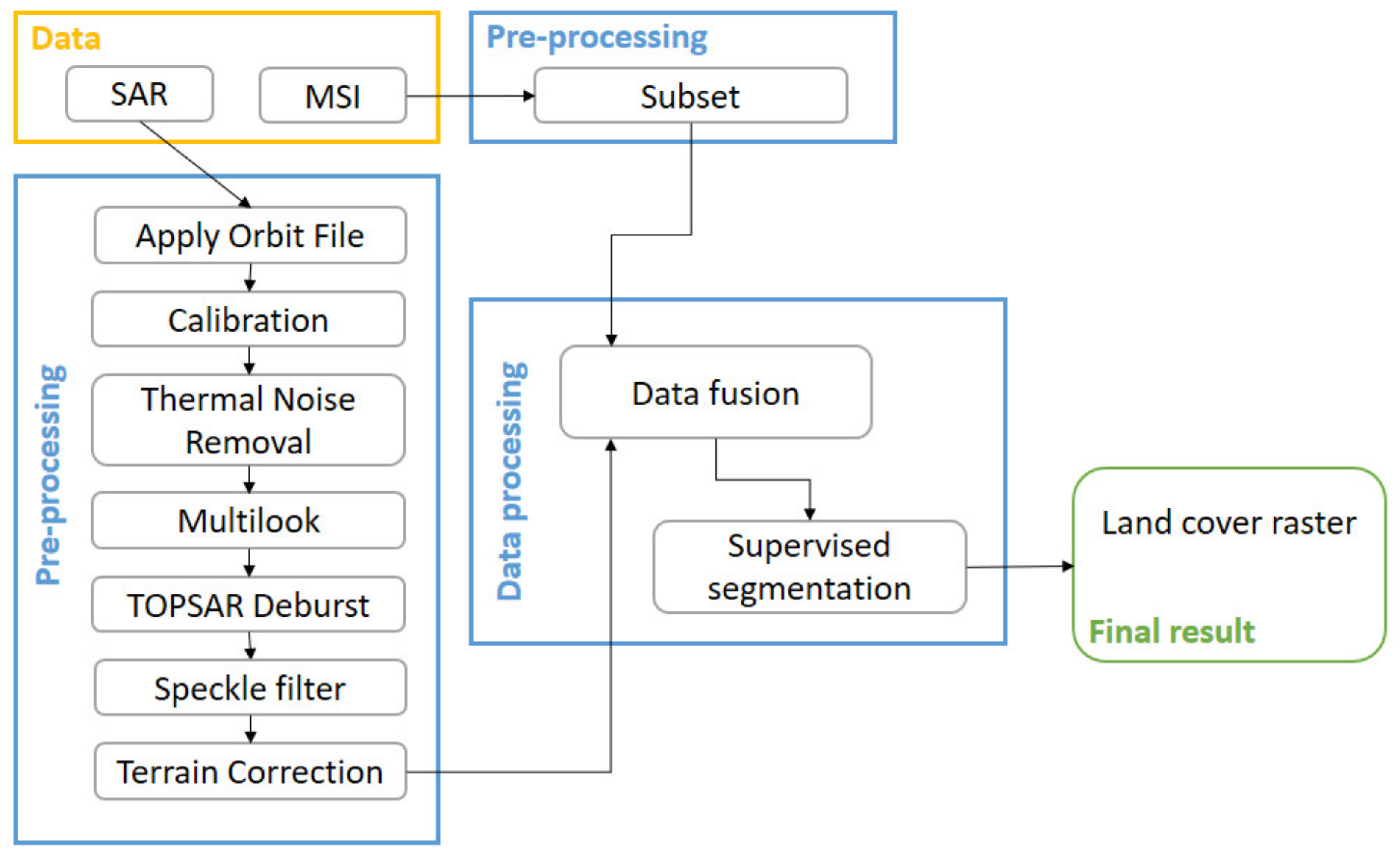
3.2.3. SAR and MSI Fusion Technique
3.2.4. Image Fusion Technique with Additional Indexes
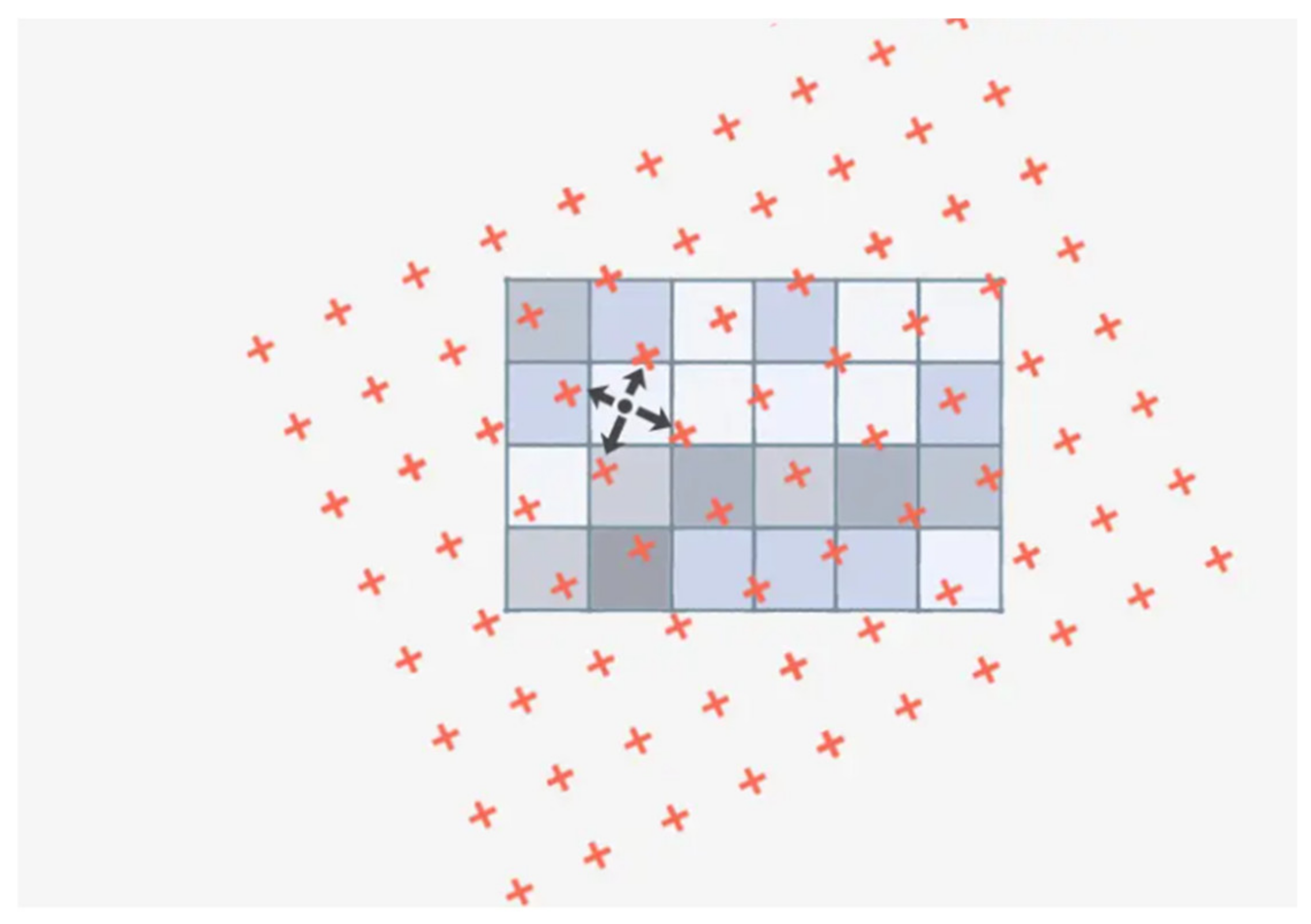
3.3. Image Segmentation and Identification of Land Cover Change
4. Results
4.1. Data Segmentation and Comparison Results
4.2. Results of Change Assessment
5. Discussion and Conclusions
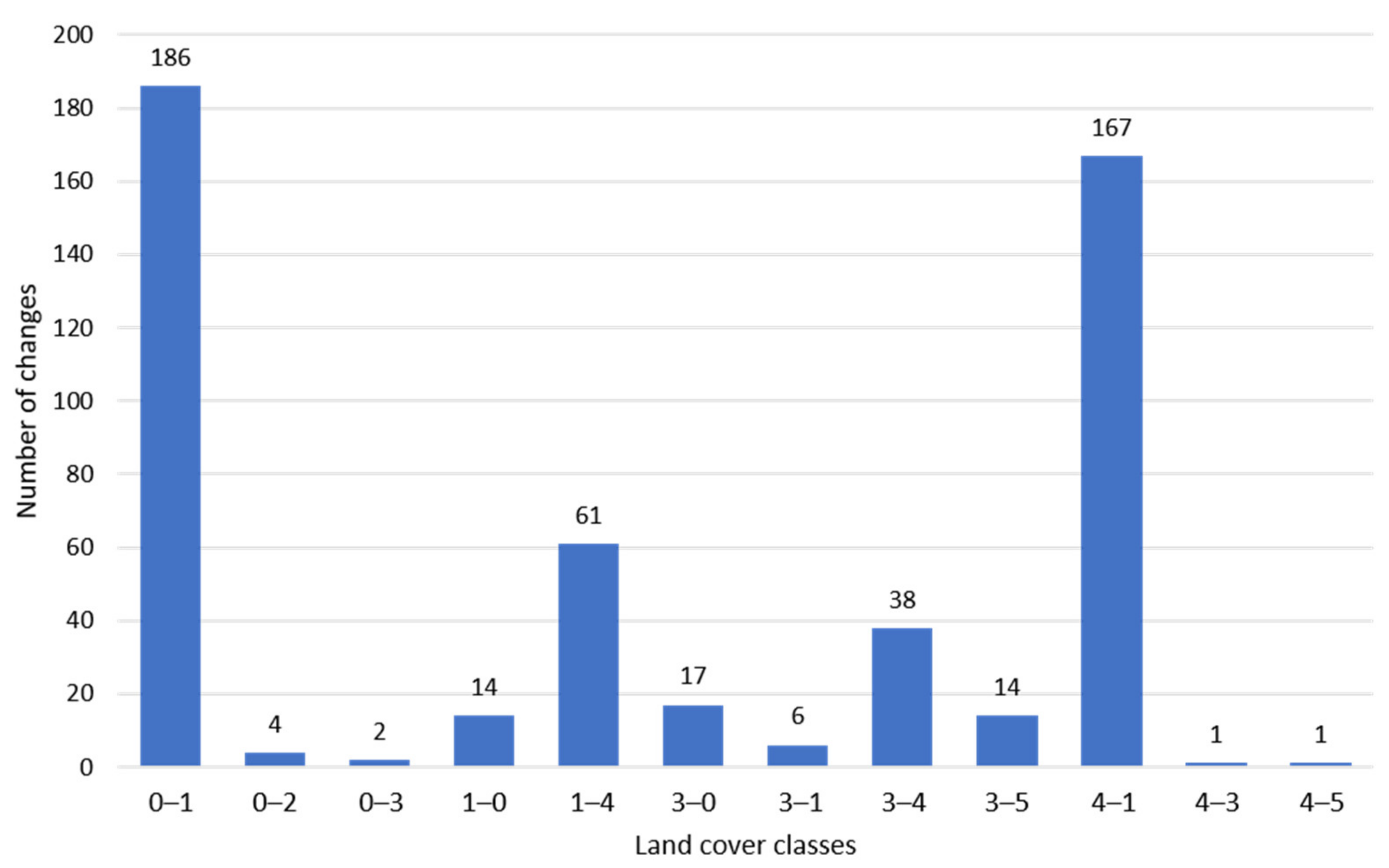
- After preprocessing and coherence extraction of the SAR and the two-period images, the result is only relevant for the initial inspection of area changes and the detection of the most altered areas.
- The results from using the second method show that the individual segmentation of SAR and MSI images differs drastically, and the field studies and accuracy estimation required the evaluation of reliability.
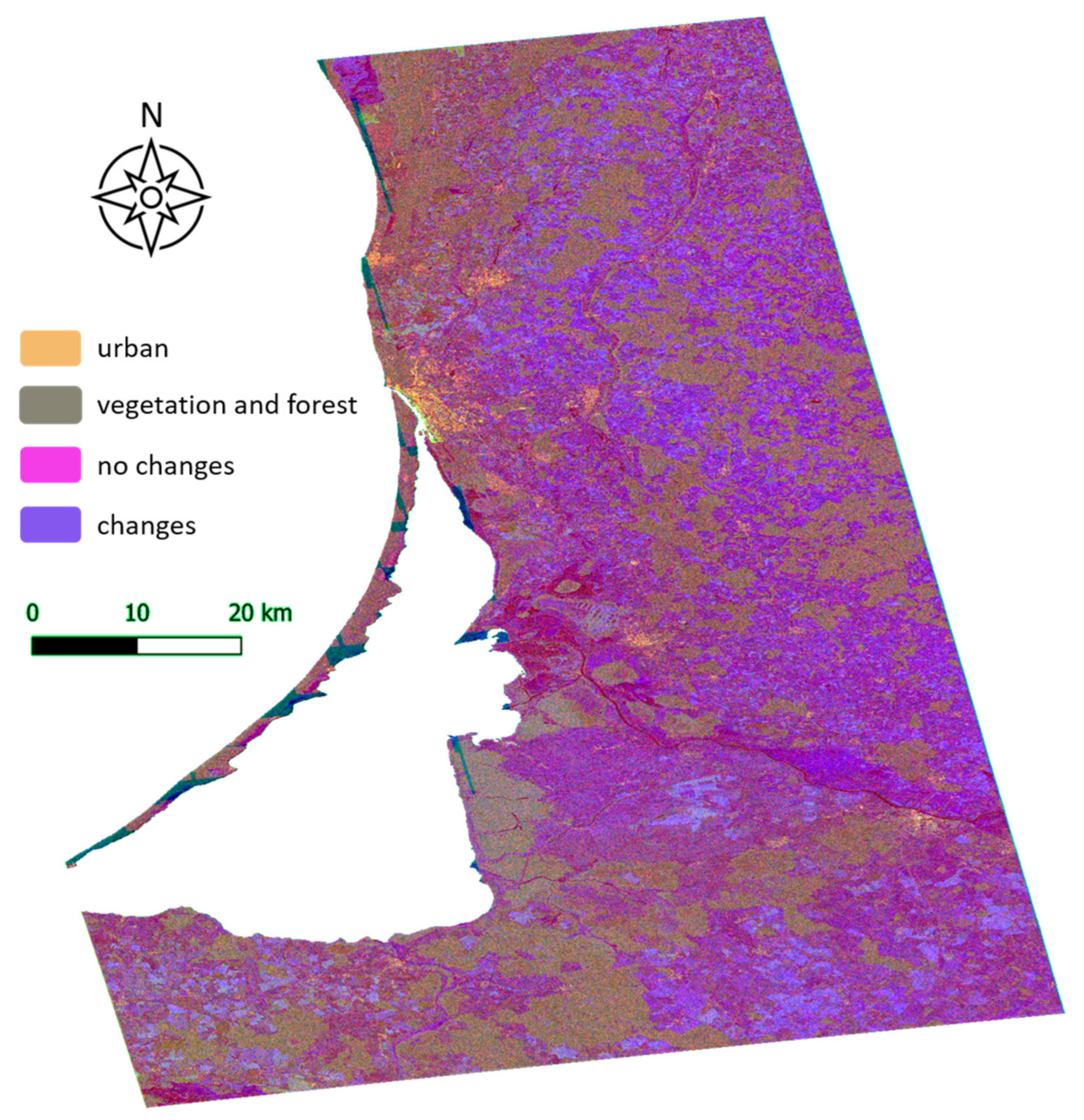
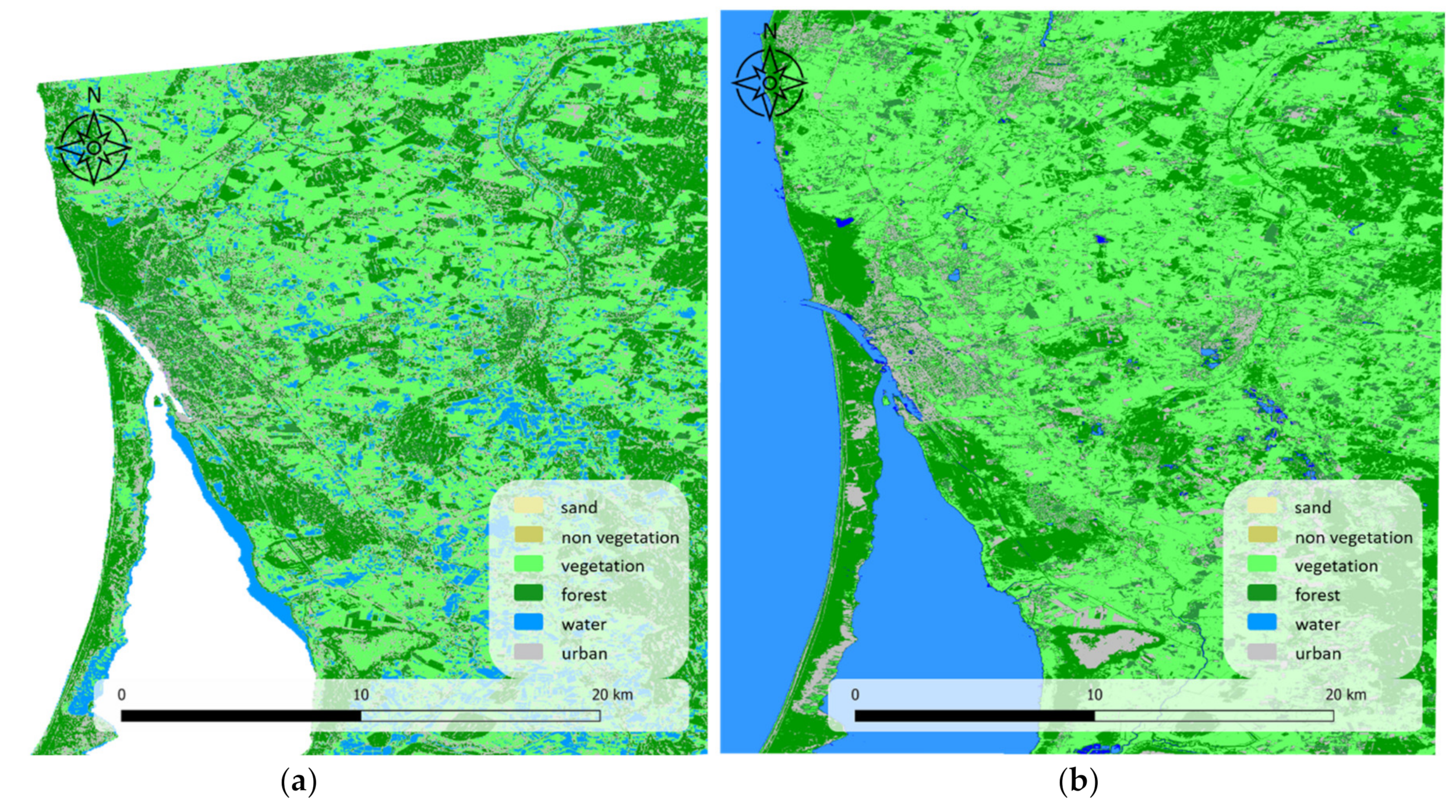
- The result of segmentation of the combined SAR and MSI data showed that the classes of urban areas, nonvegetated areas and sandy areas are poorly separated due to a similar spectral signature. Therefore, it was decided to include NDVI, S2REP and GNDVI indices to improve accuracy and highlight the class of vegetation areas. NDBI was included to highlight the class of urban areas.
- Additional indices improved the result of segmentation, but there are still errors in identifying urban areas.
- Changes that were falsely identified during the qualitative accuracy check of the identified changes (92.08% of all changes checked) were False Positive results and no False Negative results were observed in the analysis of the images. Although changes are incorrectly identified in some identified cases, visual inspection (especially when potential locations for potential inaccuracies are known) and manual correction would still use less time than not automating all the process.
Author Contributions
Funding
Institutional Review Board Statement
Informed Consent Statement
Data Availability Statement
Acknowledgments
Conflicts of Interest
References
- Louwagie, G. Land and Soil Losing Ground to Human Activities. Available online: https://www.eea.europa.eu/articles/land-and-soil-losing-ground (accessed on 10 June 2022).
- Kalnay, E.; Cai, M. Impact of urbanization and land-use change on climate. Nature 2003, 423, 528–531. [Google Scholar] [CrossRef] [PubMed]
- Hong, C.; Burney, J.A.; Pongratz, J.; Nabel, J.E.M.S.; Mueller, N.D.; Jackson, R.B.; Davis, S.J. Global and regional drivers of land-use emissions in 1961–2017. Nature 2021, 589, 554–561. [Google Scholar] [CrossRef]
- Veteikis, D.; Piškinaitė, E. Geographical research of land use change in Lithuania: Development, directions, perspectives. (Lith.: Geografiniai žemėnaudos kaitos tyrimai Lietuvoje: Raida, kryptys, perspektyvos). Geol. Geogr. 2019, 5, 14–29. [Google Scholar] [CrossRef]
- Zhou, D.; Xiao, J.; Frolking, S.; Zhang, L.; Zhou, G. Urbanization Contributes Little to Global Warming but Substantially Intensifies Local and Regional Land Surface Warming. Earth’s Future 2022, 10, 1–19. [Google Scholar] [CrossRef]
- Comber, A.; Fisher, P.; Wadsworth, R. What is land cover? Environ. Plan. B Urban Anal. City Sci. 2005, 32, 199–209. [Google Scholar] [CrossRef] [Green Version]
- Di Gregorio, A.; Jansen, L.J.M. Land Cover Classification System (LCCS): Classification Concepts and User Manual. Environment and Natural Resources Service (SDRN) GCP/RAF/287/ITA Africover—East Africa ProjectSoil Resources, Management and Conservation Service (AGLS). Available online: https://www.researchgate.net/publication/229839605_Land_Cover_Classification_System_LCCS_Classification_Concepts_and_User_Manual (accessed on 10 June 2022).
- European Enviroment Agency. Land Cover Copernicus Global Land Service. Available online: https://land.copernicus.eu/global/products/lc (accessed on 10 June 2022).
- Lambin, E.F.; Geist, H.; Rindfuss, R.R. Land-Use and Land-Cover Change. In Local Processes and Global Impacts; Springer: Berlin/Heidelberg, Germany, 2008. [Google Scholar]
- Briassoulis, H. Factors influencing land-use and land-cover change. Land Use Land Cover. Soil Sci. 2009, 1, 126–143. [Google Scholar]
- Mustard, J.F.; Defries, R.S.; Fisher, T.; Moran, E. Land-Use and Land-Cover Change Pathways and Impacts. In Land Change Science; Remote Sensing and Digital Image Processing; Springer: Dordrecht, Netherlands, 2012; pp. 411–429. [Google Scholar] [CrossRef]
- Brown, D.; Polsky, C.; Bolstad, P.V.; Brody, S.D.; Hulse, D.; Kroh, R.; Loveland, T.; Thomson, A.M. Land Use and Land Cover Change; US Department of Energy: Richland, WA, USA, 2014.
- Hartvigsen, M. Land reform and land fragmentation in Central and Eastern Europe. Land Use Policy 2014, 36, 330–341. [Google Scholar] [CrossRef]
- Feranec, J.; Soukup, T.; Taff, G.N.; Stych, P.; Bicik, I. Overview of Changes in Land Use and Land Cover in Eastern Europe. In Land-Cover and Land-Use Changes in Eastern Europe after the Collapse of the Soviet Union in 1991; Springer: Cham, Switzerland, 2017; pp. 13–33. [Google Scholar] [CrossRef]
- Loveland, T.; Sleeter, B.M.; Wickham, J.; Domke, G.; Herold, N.; Wood, N. Land Cover and Land-Use Change. In Impacts, Risks, and Adaptation in the United States: Fourth National Climate Assessment; U.S. Global Change Research Program: Washington, DC, USA, 2018; Volume II, pp. 202–231. [Google Scholar] [CrossRef]
- Rimal, B.; Sharma, R.; Kunwar, R.; Keshtkar, H.; Stork, N.E.; Rijal, S.; Rahman, S.A.; Baral, H. Effects of land use and land cover change on ecosystem services in the Koshi River Basin, Eastern Nepal. Ecosyst. Serv. 2019, 38, 100963. [Google Scholar] [CrossRef]
- Nayak, S.; Mandal, M. Impact of land use and land cover changes on temperature trends over India. Land Use Policy 2019, 89, 104238. [Google Scholar] [CrossRef]
- Tadese, M.; Kumar, L.; Koech, R.; Kogo, B.K. Mapping of land-use/land-cover changes and its dynamics in Awash River Basin using remote sensing and GIS. Remote Sens. Appl. Soc. Environ. 2020, 19, 100352. [Google Scholar] [CrossRef]
- Guo, Y.; Fang, G.; Xu, Y.P.; Tian, X.; Xie, J. Identifying how future climate and land use/cover changes impact streamflow in Xinanjiang Basin, East China. Sci. Total Environ. 2020, 710, 136275. [Google Scholar] [CrossRef]
- Li, Z.; Shen, Y.; Huang, N.; Xiao, L. Supervised classification of hyperspectral images via heterogeneous deep neural networks. In Proceedings of the International Geoscience and Remote Sensing Symposium (IGARSS), Fort Worth, TX, USA, 23–28 July 2017; pp. 1812–1815. [Google Scholar] [CrossRef]
- Ribokas, G. The Problem of Derelict Land (Soils) in Sparsely Populated Areas. (In lith.: Apleistų Žemių (Dirvonų) Problema Retai Apgyventose Teritorijose). 2011, pp. 298–307. Available online: https://vb.mab.lt/object/elaba:6228786/6228786.pdf (accessed on 10 June 2022).
- Pandit, V.R.; Bhiwani, R.J. Image Fusion in Remote Sensing Applications: A Review. Int. J. Comput. Appl. 2015, 120, 22–32. [Google Scholar] [CrossRef]
- Paris, C.; Bruzzone, L. A three-dimensional model-based approach to the estimation of the tree top height by fusing low-density LiDAR data and very high resolution optical images. IEEE Trans. Geosci. Remote Sens. 2015, 53, 467–480. [Google Scholar] [CrossRef]
- Simoes, M.; Bioucas-Dias, J.; Almeida, L.B.; Chanussot, J. A convex formulation for hyperspectral image superresolution via subspace-based regularization. IEEE Trans. Geosci. Remote Sens. 2015, 53, 3373–3388. [Google Scholar] [CrossRef] [Green Version]
- Vivone, G.; Alparone, L.; Chanussot, J.; Mura, M.D.; Garzelli, A.; Member, S.; Licciardi, G.A.; Restaino, R.; Wald, L. A Critical Comparison Among Pansharpening Algorithms. IEEE Trans. Geosci. Remote Sens. 2015, 53, 2565–2586. [Google Scholar] [CrossRef]
- Gasmi, A.; Gomez, C.; Chehbouni, A.; Dhiba, D.; Elf, H. Satellite Multi-Sensor Data Fusion for Soil Clay Mapping Based on the Spectral Index and Spectral Bands Approaches. Remote Sens. 2022, 14, 1103. [Google Scholar] [CrossRef]
- Munir, A.; Blasch, E.; Kwon, J.; Kong, J.; Aved, A. Artificial Intelligence and Data Fusion at the Edge. IEEE Aerosp. Electron. Syst. Mag. 2021, 36, 62–78. [Google Scholar] [CrossRef]
- Barbedo, J.G.A. Data Fusion in Agriculture: Resolving Ambiguities and Closing Data Gaps. Sensors 2022, 22, 2285. [Google Scholar] [CrossRef]
- Kussul, N.; Skakun, S.; Kravchenko, O.; Shelestov, A.; Gallego, J.F.; Kussul, O. Application of Satellite Optical and SAR Images for Crop Mapping and Erea Estimation in Ukraine. Inf. Technol. Knowl. 2013, 7, 203–211. [Google Scholar]
- Clerici, N.; Valbuena Calderón, C.A.; Posada, J.M. Fusion of Sentinel-1A and Sentinel-2A data for land cover mapping: A case study in the lower Magdalena region, Colombia. J. Maps 2017, 13, 718–726. [Google Scholar] [CrossRef] [Green Version]
- Denize, J.; Hubert-Moy, L.; Betbeder, J.; Corgne, S.; Baudry, J.; Pottier, E. Evaluation of using Sentinel-1 and -2 time-series to identify winter land use in agricultural landscapes. Remote Sens. 2019, 11, 37. [Google Scholar] [CrossRef] [Green Version]
- Mercier, A.; Betbeder, J.; Rumiano, F.; Baudry, J.; Gond, V.; Blanc, L.; Bourgoin, C.; Cornu, G.; Ciudad, C.; Marchamalo, M.; et al. Evaluation of Sentinel-1 and 2 time series for land cover classifiction of forest-agriculture mosaics in temperate and tropical landscapes. Remote Sens. 2019, 11, 979. [Google Scholar] [CrossRef] [Green Version]
- Khan, A.; Govil, H.; Kumar, G.; Dave, R. Synergistic use of Sentinel-1 and Sentinel-2 for improved LULC mapping with special reference to bad land class: A case study for Yamuna River floodplain, India. Spat. Inf. Res. 2020, 28, 669–681. [Google Scholar] [CrossRef]
- Mas, J.F. Monitoring land-cover changes: A comparison of change detection techniques. Int. J. Remote Sens. 1999, 20, 139–152. [Google Scholar] [CrossRef]
- Chase, T.N.; Pielke, R.A.; Kittel, T.G.F.; Nemani, R.R.; Running, S.W. Simulated impacts of historical land cover changes on global climate in northern winter. Clim. Dyn. 2000, 16, 93–105. [Google Scholar] [CrossRef]
- Yang, X.; Lo, C.P. Using a time series of satellite imagery to detect land use and land cover changes in the Atlanta, Georgia metropolitan area. Int. J. Remote Sens. 2002, 23, 1775–1798. [Google Scholar] [CrossRef]
- Cui, X.; Graf, H.F. Recent land cover changes on the Tibetan Plateau: A review. Clim. Chang. 2009, 94, 47–61. [Google Scholar] [CrossRef] [Green Version]
- European Commission. LUCAS: Land Use and Coverage Area frame Survey. 2018. Available online: https://esdac.jrc.ec.europa.eu/projects/lucas (accessed on 17 December 2019).
- European Commission. LUCAS 2006 (Land Use/Cover Area Frame Survey)—Technical Reference Document C3 Classification (Land Cover & Land Use). 2009, pp. 1–53. Available online: https://ec.europa.eu/eurostat/documents/205002/769457/QR2009.pdf (accessed on 10 June 2022).
- CORINE. CORINE Land Cover Nomenclature Conversion to Land Cover Classification System. 2010. Available online: https://land.copernicus.eu/eagle/files/eagle-related-projects/pt_clc-conversion-to-fao-lccs3_dec2010 (accessed on 10 June 2022).
- Eurostat. LUCAS Land Use and Cover Area frame Survey. 2015. Available online: https://ec.europa.eu/eurostat/ramon/other_documents/index.cfm?TargetUrl=DSP_LUCAS (accessed on 17 December 2019).
- Abdikan, S.; Sanli, F.B.; Ustuner, M.; Calò, F. Land cover mapping using Sentinel-1 SAR data. Int. Arch. Photogramm. Remote Sens. 2016, XLI-B7, 757–761. [Google Scholar] [CrossRef]
- Muro, J.; Canty, M.; Conradsen, K.; Hüttich, C.; Nielsen, A.A.; Skriver, H.; Remy, F.; Strauch, A.; Thonfeld, F.; Menz, G. Short-term change detection in wetlands using Sentinel-1 time series. Remote Sens. 2016, 8, 795. [Google Scholar] [CrossRef] [Green Version]
- Open Access Hub. 2021. Available online: https://scihub.copernicus.eu/ (accessed on 20 October 2021).
- ESA. Sentinel-1 Missions. 2020. Available online: https://sentinel.esa.int/web/sentinel/missions/sentinel-1 (accessed on 19 April 2020).
- Torres, R.; Snoeij, P.; Geudtner, D.; Bibby, D.; Davidson, M.; Attema, E.; Potin, P.; Rommen, B.Ö.; Floury, N.; Brown, M.; et al. GMES Sentinel-1 mission. Remote Sens. Environ. 2012, 120, 9–24. [Google Scholar] [CrossRef]
- Fitrzyk, M. Pre-processing and multi-temporal analysis of SAR time series. Coherence-intensity composites. In Proceedings of the 9th Advanced Training Course on Land Remote Sensing: Agriculture, Louvain-la-Neuve, Belgium, 16–20 September 2019. [Google Scholar]
- GISGeography. Bilinear Interpolation: Resample Image Cell Size with 4 Nearest Neighbors—GIS Geography. 2021. Available online: https://gisgeography.com/bilinear-interpolation-resampling (accessed on 22 November 2021).
- Bovik, A.C. Basic Gray Level Image Processing. In The Essential Guide to Image Processing; Academic Press: Cambridge, MA, USA, 2009; pp. 43–68. [Google Scholar] [CrossRef]
- Kriščiukaitienė, I.; Galnaitytė, A.; Namiotko, V.; Skulskis, V.; Lakis, A.; Jukna, L.; Didžiulevičius, L.; Šleinius, D.; Usvaltienė, L. Sustainable Farming Methodology (In Lithuanian: Tvaraus Ūkininkavimo Metodika). 2020. Available online: https://webcache.googleusercontent.com/search?q=cache:sGn3hVlROjUJ:https://www.laei.lt/x_file_download.php%3Fpid%3D3428+&cd=1&hl=lt&ct=clnk&gl=lt (accessed on 15 May 2020).
- He, C.; Shi, P.; Xie, D.; Zhao, Y. Improving the normalized difference built-up index to map urban built-up areas using a semiautomatic segmentation approach. Remote Sens. Lett. 2010, 1, 213–221. [Google Scholar] [CrossRef] [Green Version]
- Kuc, G.; Chormański, J. Sentinel-2 Imagery for Mapping and Monitoring Imperviousness in Urban Areas. ISPRS—Int. Arch. Photogramm. Remote Sens. Spat. Inf. Sci. 2019, XLII-1/W2, 43–47. [Google Scholar] [CrossRef] [Green Version]
- Park, B. Future Trends in Hyperspectral Imaging. NIR News 2016, 27, 25–38. [Google Scholar] [CrossRef]
- Haas, J.; Ban, Y. Sentinel-1A SAR and sentinel-2A MSI data fusion for urban ecosystem service mapping. Remote Sens. Appl. Soc. Environ. 2017, 8, 41–53. [Google Scholar] [CrossRef]
- Gerrells, N.S. Fusion of Sentinel-1B and Sentinel-2B Data for Forest Disturbance Mapping: Detection of Bark Beetle Mortality in the Southern Sierra Nevada. Master’s Thesis, California State University, Long Beach, CA, USA, 2018. [Google Scholar]
- Sun, C.; Bian, Y.; Zhou, T.; Pan, J. Using of multi-source and multi-temporal remote sensing data improves crop-type mapping in the subtropical agriculture region. Sensors 2019, 19, 2401. [Google Scholar] [CrossRef] [PubMed] [Green Version]
- VšĮ “Informatikos Mokslų Centras”. User Manual for the Data Analysis Tool DAMIS (In Lithuanian: Duomenų Analizės Įrankio DAMIS Instrukcija Naudotojui). 2015.SS. Available online: https://damis.midas.lt/docs/Vartotojo_instrukcija.pdf (accessed on 14 May 2021).
- Tavares, P.A.; Beltrão, N.E.S.; Guimarães, U.S.; Teodoro, A.C. Integration of Sentinel-1 and Sentinel-2 for Classification and LULC Mapping in the Urban Area of Belém, Eastern Brazilian Amazon. Sensors 2019, 19, 1140. [Google Scholar] [CrossRef] [Green Version]


Publisher’s Note: MDPI stays neutral with regard to jurisdictional claims in published maps and institutional affiliations. |
© 2022 by the authors. Licensee MDPI, Basel, Switzerland. This article is an open access article distributed under the terms and conditions of the Creative Commons Attribution (CC BY) license (https://creativecommons.org/licenses/by/4.0/).
Share and Cite
Metrikaityte, G.; Suziedelyte Visockiene, J.; Papsys, K. Digital Mapping of Land Cover Changes Using the Fusion of SAR and MSI Satellite Data. Land 2022, 11, 1023. https://doi.org/10.3390/land11071023
Metrikaityte G, Suziedelyte Visockiene J, Papsys K. Digital Mapping of Land Cover Changes Using the Fusion of SAR and MSI Satellite Data. Land. 2022; 11(7):1023. https://doi.org/10.3390/land11071023
Chicago/Turabian StyleMetrikaityte, Guste, Jurate Suziedelyte Visockiene, and Kestutis Papsys. 2022. "Digital Mapping of Land Cover Changes Using the Fusion of SAR and MSI Satellite Data" Land 11, no. 7: 1023. https://doi.org/10.3390/land11071023
APA StyleMetrikaityte, G., Suziedelyte Visockiene, J., & Papsys, K. (2022). Digital Mapping of Land Cover Changes Using the Fusion of SAR and MSI Satellite Data. Land, 11(7), 1023. https://doi.org/10.3390/land11071023