Ecosystem Service Responses to Land Use Change in Southern Guangzhou—The Practice of Applying Natural Resources Integrated Database for Research

Abstract

Based on the equivalent factor table of terrestrial ESV in China in 2010, this paper proposes a regionalized and interannual ESV correction method. Taking southern Guangzhou as the study area, which is located in the geometric center of the Guangdong–Hong Kong–Macao Greater Bay Area (GHM GBA), this study evaluated the ecosystem service equivalent value (ESEV) and ecosystem service value (ESV) and their changes in 2004, 2010 and 2016 and carried out grid processing, trend analysis and global/local spatial autocorrelation of the ecosystem service density (ESD) in the study area by using the Natural Resources Integrated Database of Guangdong Province (NRIDB). The results of data processing and spatial analysis computed in this study were published as Web services through the NRIDB and displayed in the visualization front-end. The results showed that (1) during 2004–2016, the urbanization process in the study area led to the expansion of built-up land, which occupied a large amount of ecological land and resulted in a decreasing trend of ESV. (2) Benefiting from socioeconomic development, the standard value volume of the ESEV (D value) kept increasing, which resulted in an increasing trend for the total ESV. (3) The spatial autocorrelation analysis results of ESD indicated that the spatial distribution of ESD in the study area had strong spatial agglomeration and positive spatial correlation. With the progress of urbanization and increases in research scale and interval distance, the spatial difference in ESD became larger over time. The research results provide a reference for the coordinated allocation of natural resources and environmental protection in the GHM GBA.

1. Introduction

The ecosystem maintains the material cycle, biodiversity and ecological balance of the earth by creating various service functions, which are the environmental foundation on which human beings depend for survival and development [1,2,3,4,5]. These utilities are the human welfare generated by the combination of nonnatural capital and ecosystem services that are composed of the energy flow, material flow and information flow of natural capital [6,7]. As the spatial carrier of natural ecosystems and their service functions, land is the most fundamental material basis for human survival and development [8]. Land use is the closest link between humans and nature and closely links human society and the natural ecological environment [9,10,11,12,13,14,15]. In the process of urbanization, changes in land use modes and patterns affect changes in urban and rural spaces and the ecosystem structure, which in turn affect ecosystem productivity and ecosystem services. The land use changes caused by urbanization have led to problems such as human disturbance and destruction of the structure and function of natural ecosystems and an imbalance of ecosystem services and potential ecological risks [12,13,14,15,16,17,18,19]. The essence of these problems is the contradiction between economic development and natural ecological protection. Under the background of the development goal of ecological civilization and the development strategy of new green urbanization proposed by China, the quantitative evaluation of ecosystem services in urbanized areas is the basis for the efficient and rational allocation of competitive environmental resources [20], as well as the decision basis for formulating natural resource development and utilization and ecological environment construction policies and promoting the healthy and sustainable development of cities [21].

Compared with ecosystem service value (ESV) evaluation methods based on physical quantity, the equivalent factor method (EFM) is suitable for quickly estimating the ESV by taking the accurate equivalent factor table as the core [22,23,24]. Referring to the physical quantity-based estimation method and its estimation results, Xie et al. [24] proposed an improved EFM for ESV estimation with a meta-analysis, which is easy to operate, allows easy comparison of results and is suitable for ESV estimation at certain regional scales [9]. Many researchers have directly applied the average ESV per unit area proposed by Costanza [1,2] or Xie et al. [22,23,24] to estimate the ESV at various scales in China [25]. There are few studies on the adjustment of ESV coefficients considering the actual situation and interannual variation in specific regions. Referring to the Consumer Price Index Inflation Calculator from the U.S. Bureau of Labor Statistics, Yi et al. [26] used the benefit transfer method to adjust ESV coefficients in the San Antonio River basin and Bexar County in the USA. Peng et al. [27] proposed a simple ESV adjustment coefficient with reference to the statistical yearbook, agricultural land productivity and ecological background when evaluating green space ecological networks in Guangdong Province, China. Xu et al. [28] adjusted the ESV coefficient based on the unit area value of food products, biomass of forests and normalized difference vegetation index (NDVI) and researched the Bohai Rim as a study area. However, the ESV is closely related to the composition, structure and quality of local ecosystems, as well as to the natural geographical location. Moreover, China has a vast territory with very large regional differences in climatic conditions, ecological background quality and ecosystem structure, and the economic development level among different regions is extremely unbalanced, resulting in significant differences in the ecosystem service capacity and the economic value of various ecosystem types between different regions. Therefore, it is necessary to modify Xie’s equivalent factor table both regionally and interannually.

Spatial correlation and spatial heterogeneity generally exist in the spatial pattern of geographic objects [29,30,31]. As a branch of spatial analysis, spatial autocorrelation analysis is an important method used to quantitatively analyze spatial patterns and explore the correlation degree of spatial variables [32]. The elements of ecosystems and their ecological processes are unevenly distributed in space and are complexly changeable in space–time series [33]. The distribution of human activities and their interactions with ecosystems have the characteristics of spatial differentiation; thus, the ESV is directly related to the distribution of regional physical and geographical factors and socioeconomic development [9]. As these factors all have geographical characteristics of spatial heterogeneity, such as various geographic entities, the ESV has a certain spatial correlation, making it suitable to apply spatial autocorrelation analysis and other geostatistical analysis methods [34]. However, many previous studies have focused on the spatial distribution of the ESV in their study area. Few studies have quantitatively studied the spatial clustering and spatial pattern changes of the ESV, and some studies have neglected spatial and temporal differentiation, dynamics and the nonlinear correlation of ecosystem services [35,36]. Therefore, quantitatively analyzing the spatial distribution patterns and correlation characteristics of multiple annual ESVs at the regional scale is helpful for understanding the spatial pattern characteristics of ecosystems in the study area and revealing the influencing factors and driving mechanisms of ESV changes.

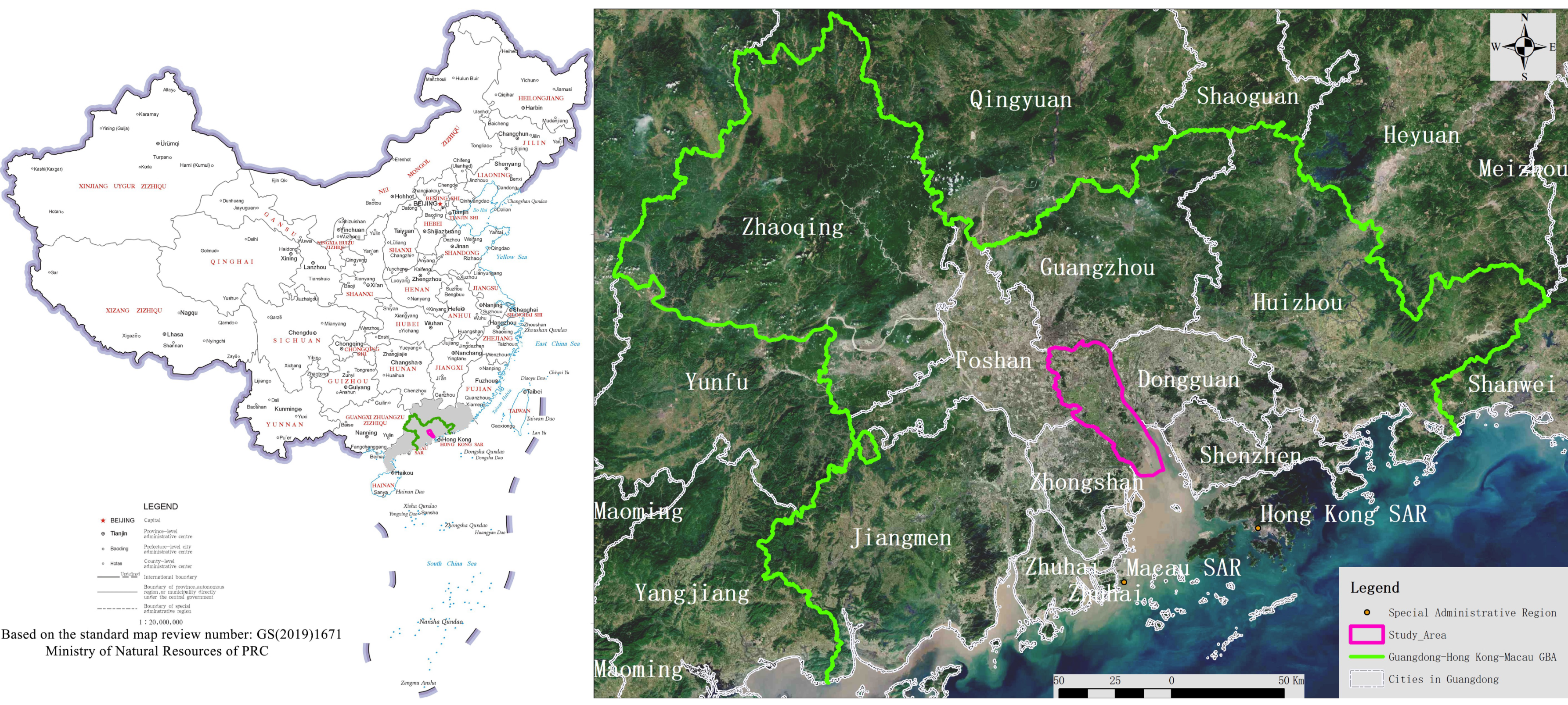
This study focused on southern Guangzhou, which is a typical urban fringe area located in the Pearl River Delta (PRD) urban agglomeration of southern China, as well as the geometric heartland of the Guangdong–Hong Kong–Macao Greater Bay Area (GHM). Since the 21st century, due to rapid urbanization and rapid economic and social development, land use in the study area has undergone tremendous changes, which may significantly affect ecosystem services and functions. Taking Guangdong Province as an example, the ecosystem service equivalent value (ESEV) and its standard value volume (D value) in Guangdong Province in 2004, 2010 and 2016 were revised. The revised ESEV and D values were applied to the ESV evaluation in the study area through a series of analysis processes, such as grid analysis, trend analysis and spatial autocorrelation analysis, to conduct a quantitative study on the spatial and temporal characteristics and regularities of ESV and the impact of built-up expansion on the spatial differentiation of ESV in the process of rapid urbanization in a typical urban fringe area, such as the study area.

As the field of natural resource management and the ecological environment become increasingly extensive and in-depth, the research content and data types are becoming increasingly rich and diverse, the volume of data for spatial analysis, calculation and management is also increasing, and the demand for data sharing is growing. Traditional stand-alone GIS software cannot support the collection, management, spatial analysis, calculation, sharing and visualization of multisource data. Therefore, we introduce the NRIDB to support the research in this paper, which is designed for natural resource big data management and service. The NRIDB is a server-side + web-side GIS that integrates technologies such as Geospatial Database Cluster, Spatio-Temporal Big Data Engine, Spatial Analysis Computing Cluster and Micro-Service Cluster.

2. Study Area, Data and Methodology

2.1. Study Area

This research focused on the southern part of Guangzhou as the study area, including Panyu District and Nansha District, with a geographic range of 113°14′ E–113°45′ E, 22°32′ N–23°05′ N and an area of 1340 km². As shown in Figure 1, located in the Western Pearl River Estuary, the study area is the geometric center, and the traffic junction of the Guangdong–Hong Kong–Macao Greater Bay Area (GHM GBA) city cluster is adjacent to Hong Kong and Macao and crosses the sea from Southeast Asia. The study area is located in the subtropical monsoon climate zone with a mild climate and an average annual rainfall amount up to 1600 mm. The topography is mainly delta plain, and a few low hills are distributed in the central and southern regions. Superior climatic conditions and the unique location of the estuary, the dense channel of the Pearl River, the geographical characteristics of the river–sea interface, the rich wetlands and other ecological factors cause the study area to have excellent natural endowments and extremely rich ecological resources. The ecosystem of the study area plays an important role in maintaining the ecological balance of the Pearl River Estuary and safeguarding the sound ecological network in GHM. Nansha Wetland Park, Huangshanlu Forest Park, 18 Luohan Mountain Forest Park, Changlong Tourist Resort and Lianhua Mountain are all famous ecological tourism areas in the study area.

2.2. Land Use Data

The land use data in this paper are based on scientific research data from Guangzhou University. These land use data are supervised by support vector machine (SVM) from Landsat 5 Thematic Mapper (TM) images in 2004 and 2010 and Landsat 8 Operational Land Imager (OLI) images in 2016. Land use was reclassified into 8 types, and the classification standard according to “the Contents and Indicators of Basic Geographic Monitoring (GQJC03-2017)” issued by the State Bureau of Surveying and Mapping Geographic Information of China is shown in

Table 1. Land use categories in the study area.

land Use Types	Definition
Built-up	Buildings, structures, road surfaces and other artificially hardened surfaces.
Cropland	After reclamation, planting food crops and constantly cultivated land.
Forest	Land covered by trees and dominated by crown canopy.
Grassland	Land covered by contiguous herbs.
Orchard	After reclamation, planting economic crops and constantly cultivated land, as well as intensive management of tea garden, orchard, garden and nursery.
Unused and other	Various bare surfaces, artificial dumps, unused land and other land use.
River	A river course with fluid water throughout the year.
Wetland and lakes	Lakes, ponds, reservoirs, wetlands and other water bodies with relatively weak liquidity.

. After partial correction of the SVM-supervised classification results, the accuracy of random sampling of land use patches was better than 90%.

2.3. Data Consolidation

To meet the study requirements, we undertook the following steps for data consolidation:

(1)

Searched agricultural data such as planting area and yield of main crops, as well as data on rainfall, surface runoff, GDP and tourism industry output in each study year from many years of the China Statistical Yearbook [37,38,39]; the Guangdong Statistical Yearbook ([40,41,42], http://tjnj.gdstats.gov.cn:8080/tjnj/2005/, accessed on 30 November 2021, http://tjnj.gdstats.gov.cn:8080/tjnj/2011/, accessed on 30 November 2021, http://tjnj.gdstats.gov.cn:8080/tjnj/2017/, accessed on 30 November 2021); and other statistics to calculate the various modified coefficients proposed in this paper. The standard value volume of ESEV in each study year was calculated based on the abovementioned agricultural statistics, combined with the crop benefit data for each year in the Agricultural Products Cost Return Assembly of China and Guangdong Province [43,44,45].

(2)

Downloaded the GPP raw data for 2004, 2010 and 2016 from the National Earth System Science Data Sharing Infrastructure, National Science & Technology Infrastructure of China (http://www.geodata.cn, accessed on 30 November 2021) [46]. The GPP data for each year were processed by the Computing Center in the NRIDB, and the total GPP of China and Guangdong Province was obtained for each study year.

The Data Center in the NRIDB aggregated and stored these data in a geospatial relational database. The Computing Center extracted data from the geospatial relational database and performed a series of spatial analysis computations.

2.4. Estimation of ESV

Costanza et al. [1] proposed an ESV accounting method based on the classification of ecosystems and service functions and estimated the global ESV. Based on Costanza et al.’s parameters, Xie et al. [22] extracted the ESEV and modified the value coefficients of the Chinese terrestrial ecosystem. With deeper research, Xie et al. [24] supplemented the ESEV according to different types of literature research and ecological monitoring data and proposed an integrated method for evaluating the ESEV in a unit area for different ecosystem types and different ecosystem service functions on Chinese terrestrial ESV. Based on the 2010 ESEV proposed by Xie et al. [24], this paper adjusts it into

Table 2. Basic reference standard ecosystem service equivalent value (ESEV) table [24].

	Category	Cropland	Orchard	Forest	Grassland	Unused and Other	River	Wetland and Lakes
Function
FP		1.36	1.035	0.29	0.38	0	0.44	0.51
RMP		0.4	0.61	0.66	0.56	0	0.23	0.5
WP		0.02	0.325	0.34	0.31	0	3.12	1.32
GR		1.11	2.07	2.17	1.97	0.02	0.77	1.1
CR		0.57	5.855	6.5	5.21	0	2.29	3.6
EP		0.17	1.825	1.93	1.72	0.1	2.55	2.6
HR		2.72	4.28	4.74	3.82	0.03	20.8	14.23
SFR		1.03	2.525	2.65	2.4	0.02	0.66	1.2
NC		0.12	0.19	0.2	0.18	0	0.07	0.18
BP		0.13	2.295	2.41	2.18	0.02	1.88	3.32
AS		0.06	1.01	1.06	0.96	0.1	0.66	2.73
Total		7.69	22.02	22.95	19.69	0.29	33.47	31.29

as the basic reference standard. In the Table 2, the provisioning services include food production (FP), raw material production (RMP) and water provision (WP); the regulation services include gas regulation (GR), climate regulation (CR), environmental purification (EP) and hydrology regulation (HR); the supporting services include soil formation and retention (SFR), nutrition circulation (NC) and biodiversity protection (BP); and the culture services mainly manifest as aesthetic scenery (AS). (Note: Considering that the study area is located in the tropical monsoon climate area, cropland is dominated by paddy fields, so the ESEV of cropland adopts paddy fields. In the original paper [24], the WP of the paddy field is negative, but in fact the study area has abundant rainfall, in addition to the water resources consumed by the paddy field itself, the paddy field can still generate a net water provision, so we adjusted the WP of the paddy field ESEV to 0.02).

Ecosystem service capacity refers to the capacity to provide ecosystem products and services in specific areas over a specific time period. Ecosystems and their services have significant spatial heterogeneity and interannual differences, so their service capabilities also have significant spatial and temporal differentiation characteristics. Considering the difference between the national parameter representation area and the interannual ecological background quality characteristics, it was necessary to modify China’s nationwide ESEV.

The food production and raw material production services were quantitatively modified by the crop production coefficients (CPCs), which were calculated from the unit area output of rice, beans and potato food crops in the national and Guangdong statistical yearbooks. These crops are the main food crops both in the nation and in the study area. The CPC calculation is shown in Equation (1):

$$\{\begin{array}{c}CPC=\frac{Productio{n}_r + Productio{n}_b + Productio{n}_p}{Tota{l}_{Area}}\\ {\mathsf{\eta }}_{Food \& Material} = \frac{CP{C}_{GDyr}}{CP{C}_{CHNyr}}·\frac{CP{C}_{CHNyr}}{CP{C}_{CHN2010}}\end{array}$$

(1)

where $Productio{n}_r$, $Productio{n}_b$ and $Productio{n}_p$ are the total production of rice, beans and potato, respectively, and $Tota{l}_{Area}$ is the total planting area of rice, beans and potato. ${\mathsf{\eta }}_{Food \& Material}$ is the modified coefficient of food production and raw material production services. $CP{C}_{GDyr}$ and $CP{C}_{CHNyr}$ are the CPCs of Guangdong and the nation in the study year, respectively. As the basic reference, $CP{C}_{CHN2010}$ is the CPC of the nation in 2010.

The water provision service in land and water bodies was quantitatively modified by rainfall and surface runoff density. The calculation is shown in Equation (2):

$$\{\begin{array}{c}{\mathsf{\eta }}_{Water\left(Land\right)}=\frac{R{f}_{SAyr}}{R{f}_{CHNyr}}·\frac{R{f}_{CHNyr}}{R{f}_{CHN2010}}\\ {\mathsf{\eta }}_{Water\left(WB\right)}=\frac{SR{D}_{SAyr}}{SR{D}_{CHNyr}}·\frac{SR{D}_{CHNyr}}{SR{D}_{CHN2010}}\end{array}$$

(2)

where ${\mathsf{\eta }}_{Water\left(Land\right)}$ and ${\mathsf{\eta }}_{Water\left(WB\right)}$ are the modified coefficients of water provision services in land and water bodies, respectively. $R{f}_{SAyr}$ and $R{f}_{CHNyr}$ are the rainfall in the study area and the nation in the study year, respectively, and $R{f}_{CHN2010}$ is the rainfall in the study area in 2010 as a basic reference. $SR{D}_{SAyr}$ and $SR{D}_{CHNyr}$ are the surface runoff densities of terrestrial water areas in the study area and the nation in the study year, respectively, and $R{f}_{CHN2010}$ is the surface runoff density of terrestrial water areas in the nation in 2010 as a basic reference.

Regulation and supporting services were quantitatively modified by the gross primary productivity (GPP), which is an important indicator of the ecological background quality and the intensity of natural biological activities. The calculation is shown in Equation (3):

$${\mathsf{\eta }}_{Regulation \& Support}=\frac{GP{P}_{SAyr}}{GP{P}_{CHNyr}}·\frac{GP{P}_{CHNyr}}{GP{P}_{CHN2010}}$$

(3)

where ${\mathsf{\eta }}_{Regulation \& Support}$ is the modified coefficient of regulating and supporting services. $GP{P}_{SAyr}$ and $GP{P}_{CHNyr}$ are the GPP in the study area and the nation in the study year, respectively, and $GP{P}_{CHN2010}$ is the GPP in the nation in 2010 as a basic reference.

The cultural service was quantitatively modified by the ratio of tourism income to GDP according to Peng et al. [27]. The calculation is shown in Equation (4):

$${\mathsf{\eta }}_{Culture}=\frac{Tourism/GD{P}_{SAyr}}{Tourism/GD{P}_{CHNyr}}·\frac{Tourism/GD{P}_{CHNyr}}{Tourism/GD{P}_{CHN2010}}$$

(4)

where ${\mathsf{\eta }}_{Culture}$ is the modified coefficient of cultural services. $Tourism/GD{P}_{SAyr}$ and $Tourism/GD{P}_{CHNyr}$ are the ratios of tourism income to GDP in the study area and the nation in the study year, respectively, and $Tourism/GD{P}_{CHN2010}$ is the ratio of tourism income to GDP in the nation in 2010 as a basic reference.

Xie et al. [24] defined 1 standard value volume of ESEV as the “D value”, which represents the economic benefit of annual grain yield in 1 unit area of cropland. The calculation process of the D value is given in Equation (5):

$$D_{yr}=\frac{S_{r-yr}\times F_{r-yr}+S_{b-yr}\times F_{b-yr}+S_{p-yr}\times F_{p-yr}}{S_{r-C2010}\times F_{r-C2010}+S_{b-C2010}\times F_{b-C2010}+S_{p-C2010}\times F_{p-C2010}}\times D_{c-2010}$$

(5)

where $D_{yr}$ represents 1 standard value volume of the ESEV in each study year for the study area (${10}^3\mathrm{Yuan}·{\mathrm{km}}^{-2}·{\mathrm{a}}^{-1}$), and $D_{c-2010}$ represents 1 standard value volume of the ESEV in 2010 for the nation (according to Xie et al. [24], $D_{c-2010}=3.4065\times {10}^3\mathrm{Yuan}·{\mathrm{hm}}^{-2}·{\mathrm{a}}^{-1}$). $S_{r-yr}$, $S_{b-yr}$ and $S_{p-yr}$ are the planting areas of rice, beans and potato accounting for the percentage of the total area of the 3 crops in the study year, respectively; $F_{r-yr}$, $F_{b-yr}$ and $F_{p-yr}$ are the economic benefits per unit area of rice, beans and potato in the study year for the study area, respectively. $S_{r-C2010}$, $S_{b-C2010}$ and $S_{p-C2010}$ are the planting areas of rice, beans and potato, respectively, accounting for the percentage of the total area of the 3 crops in 2010 for the nation; $F_{r-C2010}$, $F_{b-C2010}$ and $F_{p-C2010}$ are the economic benefits per unit area of rice, beans and potato in 2010 for the nation, respectively.

The ecosystem service estimation process is given in Equations (6)–(8):

$${\mathit{ESEV}}_{\mathit{yr}\_\mathit{kf}}={\mathsf{\eta }}_{\mathit{yr}\_\mathit{kf}}\times {\mathit{ESEV}}_{\mathit{CHN}2010\_\mathit{kf}}$$

(6)

$$ESE{V}_{yr\_k}={\displaystyle \sum }_{f}ESE{V}_{yr\_kf}$$

(7)

$$ES{V}_{yr}=D_{yr}\times {\displaystyle \sum }_{k}ESE{V}_{yr\_k}\times A_k$$

(8)

where $ESE{V}_{yr\_kf}$ refers to the ESEV of each ecosystem service function “f” and land use type “k” in the study year; $ESE{V}_{yr\_k}$ refers to the total ESEV of each land use type “k” in the study year (the total item in

Table 3. The annual modified coefficients for ecosystem service functions.

		FP	RMP	WP	GR	CR	EP	HR	SFR	NC	BP	AS
Land	2004	1.03	1.03	2.6	1.62	1.62	1.62	1.62	1.62	1.62	1.62	2.13
	2010	1.07	1.07	2.74	1.86	1.86	1.86	1.86	1.86	1.86	1.86	2.11
	2016	1.12	1.12	3.41	1.53	1.53	1.53	1.53	1.53	1.53	1.53	3.55
Water	2004	1.98	1.98	3.03	1.62	1.62	1.62	1	1.62	1.62	1.62	2.13
	2010	1.9	1.9	3.46	1.86	1.86	1.86	1	1.86	1.86	1.86	2.11
	2016	1.92	1.92	4.28	1.53	1.53	1.53	1	1.53	1.53	1.53	3.55

); $ESE{V}_{CHN2010\_kf}$ refers to the ESEV of each ecosystem service function “f” and land use type “k” in 2010 for the nation, which was the basic reference, as shown in Table 2; and ${\mathsf{\eta }}_{yr\_kf}$ is the annual modified coefficients of each ecosystem service function “f” and land use type “k”, calculated using Equations (1)–(5), and the results are compiled in

Table 4. Land use changes in the study area.

Land Use Categories	2004		2010		2016		2004–2016
	$\mathbf{Area}\left(\mathbf{h}{\mathbf{m}}^2\right)$	%	$\mathbf{Area}\left(\mathbf{h}{\mathbf{m}}^2\right)$	%	$\mathbf{Area}\left(\mathbf{h}{\mathbf{m}}^2\right)$	%	$\mathbf{Area}\left(\mathbf{h}{\mathbf{m}}^2\right)$	%	% yr
Built-up	35,108.1	26.19	39,093.85	29.17	40,518.61	30.23	5411	15.41	1.2
Cropland	26,084.3	19.46	24,681.73	18.41	24,169.38	18.03	−1915	−7.34	−0.63
Forest	4547.71	3.39	5985.44	4.47	6135.92	4.58	1588	34.92	2.53
Grassland	126.4	0.09	1308.64	0.98	1083.88	0.81	957	757.5	19.61
Orchard	17,707.32	13.21	7861.43	5.87	7478.9	5.58	−10228	−57.76	−6.93
Unused and other	808.05	0.6	4983.58	3.72	5000.79	3.73	4193	518.87	16.4
River	35,974.58	26.84	29,326.22	21.88	29,152.83	21.75	−6822	−18.96	−1.74
Wetland and lakes	13,678.86	10.21	20,794.43	15.51	20,495.01	15.29	6816	49.83	3.43
Total	134,035.3	-	134,035.3	-	134,035.3	-	-	-	-

. $ES{V}_{yr}$ is the total ESV of each ecosystem service function and land use type in the study year (

Table 5. The ESEV of various land use and ecosystem service functions.

Type	Year	Cropland	Orchard	Forest	Grassland	Unused and Other	River	Wetland and Lakes
FP	2004	1.4	1.07	0.3	0.39	0	0.87	1.01
	2010	1.46	1.11	0.31	0.41	0	0.84	0.97
	2016	1.52	1.16	0.32	0.43	0	0.84	0.98
RMP	2004	0.41	0.63	0.68	0.58	0	0.46	0.99
	2010	0.43	0.65	0.71	0.6	0	0.44	0.95
	2016	0.45	0.68	0.74	0.63	0	0.44	0.96
WP	2004	0.05	0.85	0.88	0.81	0	9.45	4
	2010	0.05	0.89	0.93	0.85	0	10.8	4.57
	2016	0.07	1.11	1.16	1.06	0	13.35	5.65
GR	2004	1.8	3.35	3.52	3.19	0.03	1.25	1.78
	2010	2.06	3.85	4.04	3.66	0.04	1.43	2.05
	2016	1.7	3.17	3.32	3.01	0.03	1.18	1.68
CR	2004	0.92	9.49	10.53	8.44	0	3.71	5.83
	2010	1.06	10.89	12.09	9.69	0	4.26	6.7
	2016	0.87	8.96	9.95	7.97	0	3.5	5.51
EP	2004	0.28	2.96	3.13	2.79	0.16	4.13	4.21
	2010	0.32	3.39	3.59	3.2	0.19	4.74	4.84
	2016	0.26	2.79	2.95	2.63	0.15	3.9	3.98
HR	2004	4.41	6.93	7.68	6.19	0.05	20.8	14.23
	2010	5.06	7.96	8.82	7.11	0.06	20.8	14.23
	2016	4.16	6.55	7.25	5.84	0.05	20.8	14.23
SFR	2004	1.67	4.09	4.29	3.89	0.03	1.07	1.94
	2010	1.92	4.7	4.93	4.46	0.04	1.23	2.23
	2016	1.58	3.86	4.05	3.67	0.03	1.01	1.84
NC	2004	0.19	0.31	0.32	0.29	0	0.11	0.29
	2010	0.22	0.35	0.37	0.33	0	0.13	0.33
	2016	0.18	0.29	0.31	0.28	0	0.11	0.28
BP	2004	0.21	3.72	3.9	3.53	0.03	3.05	5.38
	2010	0.24	4.27	4.48	4.05	0.04	3.5	6.18
	2016	0.2	3.51	3.69	3.34	0.03	2.88	5.08
AS	2004	0.13	2.15	2.26	2.04	0.21	1.41	5.81
	2010	0.13	2.13	2.24	2.03	0.21	1.39	5.76
	2016	0.21	3.59	3.76	3.41	0.36	2.34	9.69
Total	2004	11.47	35.55	37.49	32.14	0.51	46.31	45.47
	2010	12.95	40.19	42.51	36.39	0.58	49.56	48.81
	2016	11.2	35.67	37.5	32.27	0.65	50.35	49.88

). $D_{yr}$ represents 1 standard value volume of the ESEV in each study year (${10}^3\mathrm{Yuan}·{\mathrm{hm}}^{-2}·{\mathrm{a}}^{-1}$), and $A_k$ is the total area of each land use type “k” in the study year.

2.5. Grid Processing

The grid processing mode divided the study area into a regular grid matrix of the same size and used the grid as a statistical unit in the geospatial analysis. The mode replaced the regular square grid as the spatial statistical unit of the ESEV and ESV instead of irregular land use patches, ensuring capacity invariance in the unit, not only highlighting the spatial position distribution characteristics of the ESV but also facilitating the spatialized quantitative statistics of the ESV.

In this work, the study area was divided into 200 × 200 m, 500 × 500 m, 1 km × 1 km, 2 km × 1 km and 4 km × 4 km square grids by the equal space sampling method. Spatial overlap computing was carried out by using the grid matrix and land use data for each study year to calculate the area of various land use types in each grid in each study year and calculate the total ESEV of each grid. The spatial distribution of ESEV and the ecosystem service capacity for each study year were evaluated from the spatial overlap analysis.

2.6. Global Spatial Autocorrelation Analysis

Spatial autocorrelation analysis was used to measure whether the distribution of spatial variables was agglomerated and was mainly measured by the spatial autocorrelation index. This paper used $\mathrm{Moran}’\mathrm{s\; I}$ [29,47,48] to observe the overall trend of the spatial correlation of ecosystem service capabilities across the study area. The equation of Moran’s I is given in Equation (9):

$$\mathrm{Moran}’\mathrm{s}\mathrm{I}=\frac{n{{\displaystyle \sum }}_{i=1}^n{{\displaystyle \sum }}_{j\ne 1}^n{w}_{\mathit{ij}}\left(x_i-\overline{x}\right)\left(x_j-\overline{x}\right)}{\left({{\displaystyle \sum }}_{i=1}^n{{\displaystyle \sum }}_{j=1}^n{w}_{\mathit{ij}}\right){{\displaystyle \sum }}_{i=1}^n{\left(x_i-\overline{x}\right)}^2}$$

(9)

where $n$ is the number of square grids; $x_i$ and $x_j$ represent the observations of variable $x$ in the $i$ and $j$ square grids, respectively; $\overline{x}$ is the average of variable $x$; and $w_{ij}$ is the spatial weight matrix, where $w_{ij}=1$ when $x_i$ and $x_j$ are adjacent to each other, and $w_{ij}=0$ when they are not adjacent. The value of $\mathrm{Moran}’\mathrm{s}\mathrm{I}$ is between −1 and 1; when it is less than 0, it means a negative correlation, a value equal to 0 means an irrelevant correlation, and a value greater than 0 means a positive correlation. The larger the value is, the greater the correlation of the observation values in the spatial distribution and the stronger the spatial aggregation.

2.7. Local Spatial Autocorrelation Analysis

Although global spatial autocorrelation analysis can reveal the overall dependence of the spatial distribution of ESV grid cells in the study area, it does not sufficiently reflect the spatial autocorrelation of local regional units. The local ${\mathrm{Moran}’\mathrm{s}\mathrm{I}}_i$ index [47] was used to measure the ESV spatial heterogeneity between grid cells i and j. The calculation equation is given in Equation (10):

$$\mathrm{Moran}’{\mathrm{s}\mathrm{I}}_i=\frac{\left(x_i-\overline{x}\right)}{m_0}{{\displaystyle \sum }}_j{w}_{ij}\left(x_i-\overline{x}\right)$$

(10)

where $m_0={{\displaystyle \sum }}_i{\left(x_i-\overline{x}\right)}^2/n$. The meanings of $x_i$, $x_j$, $w_{ij}$ and $w_{ij}$ are the same as above. When ${\mathrm{Moran}’\mathrm{s}\mathrm{I}}_i>0$, it indicates that the spatial distribution of elements presents high–high-type agglomeration or low–low-type agglomeration. When ${\mathrm{Moran}’\mathrm{s}\mathrm{I}}_i<0$, it indicates that the spatial distribution of elements presents a high–low-type interlaced or low–high-type interlaced distribution.

The significance test equation is given in Equation (11):

$$\mathrm{Z}\left({\mathrm{I}}_i\right)=\frac{{\mathrm{I}}_i-E\left({\mathrm{I}}_i\right)}{\sqrt{VAR\left({\mathrm{I}}_i\right)}}$$

(11)

where $\mathrm{Z}\left({\mathrm{I}}_i\right)$ represents the level of spatial autocorrelation, $E\left({\mathrm{I}}_i\right)$ represents the mathematical expectation of $\mathrm{Moran}’{\mathrm{s}\mathrm{I}}_i$, and $VAR\left({\mathrm{I}}_i\right)$ represents the variance.

3. Results

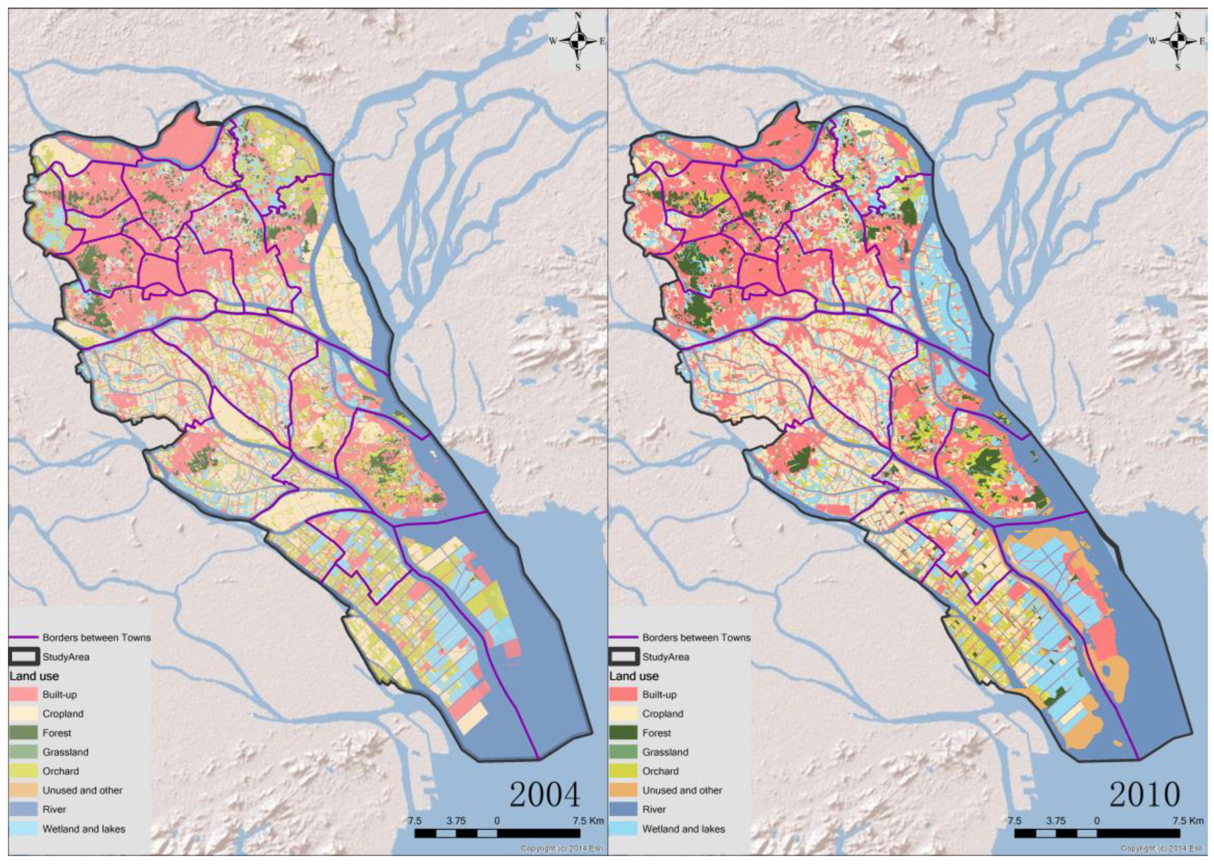
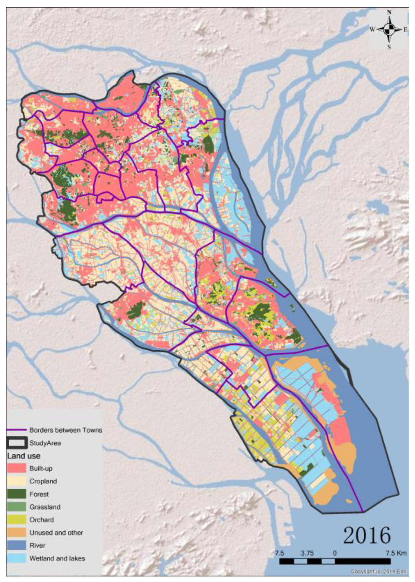
3.1. Changes in Land Use

Based on the results of land use classification in each study year, the area of built-up land in the study area greatly increased, and the area ratio increased from second place to first place, reaching 30.23%, with an average annual increase of 1.2%, reflecting the rapid progress of urbanization in southern Guangzhou during the study period. Grassland and unused and other land types had the largest growth ratio, with average annual increases of 19.61% and 16.4%, respectively. The increase in grassland was mainly located in public green areas near parks and residential areas. These grasslands are the result of Guangzhou’s green infrastructure construction in recent years. The increased unused land mainly came from reclamation construction during the recent decade, which was mostly located in Longxue Island and the 19th Creek area in the southern part of Nansha District. The urbanization process also led to a series of changes in various types of ecological land. The areas of cropland, orchard and river decreased to varying degrees, the increase in wetland area reached 49.83%, and the increase in wetland area reached 34.92%.

During the study period, the development of urbanization and industrialization was mainly to occupy cropland and orchards. In addition, a series of ecological environment constructions transformed some cropland land and orchards into forestland, grassland and wetland. The increase in forestland was mainly due to the policy of “returning cropland to forests”, in which local governments transformed low-yield cropland and orchards located in the mountains into forestland. The newly added forest area was mainly located in the protected area of ecological red lines such as Lianhua Mountain and Dafu Mountain; the forest area reduction during 2010–2016 was mainly located in Huangshanlu and Dashanna Mountain near the Nansha urban area. Most of the increased wetlands were located in Wanqingsha and Longxue Island in the central and southern parts of Nansha District, and these areas were located in the sedimentation zone of the Pearl River Estuary. The combination of delta flow and artificial cofferdams formed regular artificial land with natural conditions for the construction of wetland ecosystems. Coupled with the support of the Guangzhou government for the construction of wetland ecosystems, many wetlands were constructed in the central and southern parts of Nansha District.

3.2. The Coefficients of ESEV and ESV

Based on the abovementioned modification methods and data consolidation results, the interannual modified coefficients for each type of ecosystem service function in the study area were calculated, as shown in Table 3.

According to Equations (6) and (7), the data in Table 2 and Table 3 were calculated to obtain the ESEV of various land use and ecosystem service functions in the study area. The results are shown in Table 5.

The ESEV represents ecosystem service function and capacity, and the D value represents the level of socioeconomic development and is the proxy for converting the ESEV into the monetized ESV. Based on Xie’s et al. [24] study, we modified the D value of the study area in 2004, 2010 and 2016 as shown in Equation (5). According to our calculations from various statistics and assemblies, the modified D value in each study year was $D_{2004}=2.351\times {10}^3\mathrm{Yuan}·{\mathrm{hm}}^{-2}·{\mathrm{a}}^{-1}$, $D_{2010}=3.986\times {10}^3\mathrm{Yuan}·{\mathrm{hm}}^{-2}·{\mathrm{a}}^{-1}$ and $D_{2016}=5.416\times {10}^3\mathrm{Yuan}·{\mathrm{hm}}^{-2}·{\mathrm{a}}^{-1}$. The ESV per unit area of each land use type in each study year is shown in

Table 6. The ESV per unit area in each study year (${10}^3\mathrm{Yuan}·{\mathrm{hm}}^{-2}·{\mathrm{a}}^{-1}$ ).

Type	Year	Cropland	Orchard	Forest	Grassland	Unused and Other	River	Wetland and Lakes
FP	2004	3.29	2.52	0.71	0.92	0	2.05	2.37
	2010	5.82	4.42	1.24	1.63	0	3.35	3.87
	2016	8.23	6.28	1.73	2.33	0	4.55	5.31
RMP	2004	0.96	1.48	1.6	1.36	0	1.08	2.33
	2010	1.71	2.59	2.83	2.39	0	1.75	3.79
	2016	2.44	3.68	4.01	3.41	0	2.38	5.2
WP	2004	0.12	2	2.07	1.9	0	22.22	9.4
	2010	0.2	3.55	3.71	3.39	0	43.05	18.22
	2016	0.38	6.01	6.28	5.74	0	72.3	30.6
GR	2004	4.23	7.88	8.28	7.5	0.07	2.94	4.18
	2010	8.21	15.35	16.1	14.59	0.16	5.7	8.17
	2016	9.21	17.17	17.98	16.3	0.16	6.39	9.1
CR	2004	2.16	22.31	24.76	19.84	0	8.72	13.71
	2010	4.23	43.41	48.19	38.62	0	16.98	26.71
	2016	4.71	48.53	53.89	43.17	0	18.96	29.84
EP	2004	0.66	6.96	7.36	6.56	0.38	9.71	9.9
	2010	1.28	13.51	14.31	12.76	0.76	18.89	19.29
	2016	1.41	15.11	15.98	14.24	0.81	21.12	21.56
HR	2004	10.37	16.29	18.06	14.55	0.12	48.9	33.45
	2010	20.17	31.73	35.16	28.34	0.24	82.91	56.72
	2016	22.53	35.47	39.27	31.63	0.27	112.65	77.07
SFR	2004	3.93	9.62	10.09	9.15	0.07	2.52	4.56
	2010	7.65	18.73	19.65	17.78	0.16	4.9	8.89
	2016	8.56	20.91	21.93	19.88	0.16	5.47	9.97
NC	2004	0.45	0.73	0.75	0.68	0	0.26	0.68
	2010	0.88	1.4	1.47	1.32	0	0.52	1.32
	2016	0.97	1.57	1.68	1.52	0	0.6	1.52
BP	2004	0.49	8.75	9.17	8.3	0.07	7.17	12.65
	2010	0.96	17.02	17.86	16.14	0.16	13.95	24.63
	2016	1.08	19.01	19.99	18.09	0.16	15.6	27.51
AS	2004	0.31	5.05	5.31	4.8	0.49	3.31	13.66
	2010	0.52	8.49	8.93	8.09	0.84	5.54	22.96
	2016	1.14	19.44	20.36	18.47	1.95	12.67	52.48
Total	2004	26.97	83.59	88.16	75.56	1.2	108.88	106.89
	2010	51.63	160.2	169.45	145.05	2.32	197.54	194.57
	2016	60.66	193.18	203.1	174.78	3.51	272.69	270.16

.

3.3. The Assessment of ESEV and ESV

The process of land use change is usually accompanied by changes in the landscape pattern, landscape ecological process and ESV. By utilizing the modified ESEV, modified ESV and land use categories (Table 3, Table 5 and Table 6, respectively), the ESEV of land use type “k” and ecosystem service function type “f” and the total ESV of the study area in 2004, 2010 and 2016 could be obtained in ArcGIS and Excel using Equations (6)–(8). These results are shown in

Table 7. The total ESEV of each land use and its changes (1000 ESEV).

	Cropland	Forest	Grassland	Orchard	Unused and Other	River	Wetland and Lakes	Total
2004 ESEV	299.19	161.67	4.74	569.11	0.41	1665.98	621.98	3323.08
%	9	4.87	0.14	17.13	0.01	50.13	18.72	-
2010 ESEV	319.63	240.55	55.63	286.08	2.89	1453.41	1014.98	3373.17
%	9.62	7.24	1.67	8.61	0.09	43.74	30.54	-
2016 ESEV	270.7	218.87	40.65	241.34	3.25	1467.84	1022.29	3264.94
%	8.15	6.59	1.22	7.26	0.1	44.17	30.76	-
2004–2010 Change	20.44	78.88	50.89	−283.03	2.48	−212.57	393	50.09
Change rate (%)	6.83	48.79	1073.63	−49.73	604.88	−12.76	63.19	1.51
2010–2016 Change	−48.93	−21.68	−14.98	−44.74	0.36	14.43	7.31	−108.23
Change rate (%)	−15.31	−9.01	−26.93	−15.64	12.46	0.99	0.72	−3.21
2004–2016 Change	−28.49	57.2	35.91	−327.77	2.84	−198.14	400.31	−58.14
Change rate (%)	−9.52	35.38	757.59	−57.59	692.68	−11.89	64.36	−1.75
Annual change(%)	−0.83	2.56	19.61	−6.9	18.83	−1.05	4.23	−0.15

and

Table 8. The total ESV of each land use and its changes (million RMB).

	Cropland	Forest	Grassland	Orchard	Unused and Other	River	Wetland and Lakes	Total
2004 ESV	703.39	380.09	11.14	1337.99	0.97	3916.73	1462.27	7812.58
2010 ESV	1274.04	958.85	221.74	1140.3	11.52	5793.28	4045.69	13,445.42
2016 ESV	1466.1	1185.39	220.14	1307.12	17.6	7949.85	5536.73	17,682.93
2004–2010	570.65	578.76	210.6	−197.69	10.55	1876.55	2583.42	5632.84
Change rate (%)	81.13	152.27	1890.48	−14.78	1087.63	47.91	176.67	72.1
2010–2016	192.06	226.54	−1.6	166.82	6.08	2156.57	1491.04	4237.51
Change rate (%)	15.07	23.63	−0.72	14.63	52.78	37.23	36.86	31.52
2004–2016	762.71	805.3	209	−30.87	16.63	4033.12	4074.46	9870.35
Change rate (%)	108.43	211.87	1876.12	−2.31	1714.43	102.97	278.64	126.34

.

The ESEV is a quantitative indicator reflecting the relative service capabilities of various ecosystem services in various ecosystems. The total ESEV of the study area was approximately 3,323,080 in 2004, peaked at 3,373,170 in 2010 and declined to 3,264,940 in 2016.

As shown in Table 6 and Table 7, during the period 2004–2010, the urbanization process reduced the area of cropland and orchard in the study area; however, due to the increase in the ESEV coefficients of ecological land and the increase in the areas of forests, grasslands and wetlands, the total ESEV in the study area increased by 50,090, and the comprehensive service capacity of the ecosystem was strengthened. During the period 2010–2016, the total ESEV in the study area decreased by 108,230, a decrease of 3.21%, and the comprehensive service capacity of the ecosystem was significantly weakened, which was mainly caused by the ESEV coefficients of the land ecosystem being reduced by varying degrees, although the ESEV coefficients of the water ecosystem increased slightly. In general, during 2004–2016, the total ESEV in the study area decreased by 58,140. The urbanization process made the built-up land occupy a large amount of ecological land, and the ESEV coefficients of the land ecosystem hardly increased. Although the ESEV gains from the increase in wetland area and the ESEV coefficients of the water ecosystem were far greater than the ESEV losses from the decrease in river area, the increase in ecological land with a high service capacity, such as forest and grassland, could not offset the loss of ESEV caused by the large reduction in cropland and orchard area.

Because of the high ESEV coefficients and the large area, the ecosystem services supplied by rivers and wetlands and lakes were the highest among the eight land use categories, accounting for approximately 70% of the total ESEV. The ESEV coefficients of cropland and orchard were relatively low, and their area continued to decrease, resulting in a decrease in the ESEV share from 26% to approximately 15%. Although forests and grasslands had high ESEV coefficients and large area growth, due to the small area base, their ecosystem service capacity was relatively limited, and their role in ecosystems was increasingly important.

Combining Table 7 and Table 8, the total ESV of the study area was approximately 7.81 billion yuan in 2004, 13.45 billion yuan in 2010 and 17.68 billion yuan in 2016. During the 12-year study period, the ESV in the study area increased by 126.34%, with an increase of 72.1% in 2004–2010 and 31.52% in 2010–2016. The ESVs of cropland, forest, unused and other, river, and wetland increased by different degrees during the 12-year study period. The ESV of grassland increased explosively with the increase in area and the ESEV coefficients during 2004–2010 and decreased slightly by 0.72% during 2010–2016 due to decreases in area and ESEV coefficients. However, the overall growth rate was still as high as 1876.12% during the whole study period, which was the highest among the seven types of ecological land. The orchard area continued to decrease, and its ESV decreased by 14.78% during 2004–2010. Despite the increase in the standard value volume of the ESEV between 2010 and 2016, the ESV of orchards decreased by a net of 2.31% throughout the period, which was the only ecological land type with a net decrease in ESV.

Despite the changes in natural conditions and the process of urbanization, the reduction in ecological land may have resulted in a decline in ecosystem services. However, with the increasing value of ESEV standards promoted by socioeconomic development, the total ESV in the study area still had a large increase after offsetting the ESV losses caused by ecological background quality changes and the area reduction of ecological land.

3.4. Spatial Distribution of Ecosystem Service Density

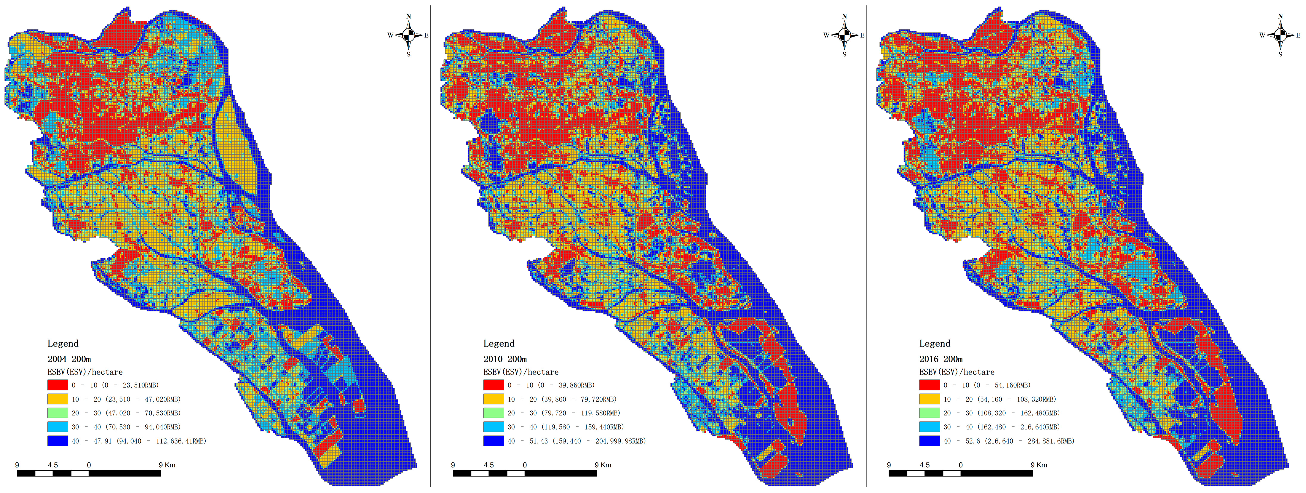
The ESEV and ESV of each land use patch for each study year were calculated based on the spatial land use data shown in Figure 2, the ESEV coefficients shown in Table 5 and the ESV coefficients shown in Table 6. Combining the land use data and 200 × 200 m, 500 × 500 m, 1 km × 1 km, 2 km × 2 km, and 4 km × 4 km square grids in the study area, the ecosystem service density (ESD, ESEV density and ESV density) in each grid was calculated by intersect analysis. The grids were reclassified into five types (lowest, lower, middle, higher and highest) by equal-spacing classification (10 ESEV as a space unit), as shown in Figure 3. As the results show in Figure 3, the high-value grids of the ESV were mainly concentrated in the southeast of the study area, and the low-value grids were concentrated in the central and northern parts. From 2004–2016, the low-value grids located in the northern part of the study area expanded linearly from west to east, and the low-value grids located in the middle of the study area increased significantly and were clustered.

The intersect analysis in the NRIDB was performed by GeoHPC cluster. During the computing process, the study area was divided into dozens of partitions and formed a computing task queue containing dozens of sub-computing tasks. Then, according to the order of the computing task queue, the land use and grid in the partition where the sub-computing task was located were sent to the GeoHPC computing node for intersect analysis. Finally, the GeoHPC cluster admin node summarized the parallel computing results of each GeoHPC computing node to form the ESD in each grid.

3.5. Trend Analysis for ESD Distribution

Figure 4 is a graph of the 1 km × 1 km ESD global trend analysis in Figure 3. Due to the small volume of data, global trend analysis computation was performed in 1 ArcGIS Engine node in the Computing Center. Figure 4 shows that the spatial distribution of ecosystem service capacity in the study area had an obvious trend effect. In the X-axis direction, there was an upward trend from west to east, and the minimum value was located in the middle of the west. In the Y-axis direction, there was an upward trend from north to south, and the minimum value was in the north-central position. Due to historical reasons, the subcenter of Guangzhou city is located in the Panyu District in the north-western part of the study area. Many rivers, wetlands and forests with strong ecological services are located in the east and south of the study area, which made the spatial distribution of the ESD decrease from the southeast to the northwest of the study area. The difference in the functional density of ecosystem services in the south–north direction of the study area was less than that in the east–west direction. With the further urbanization development of the Nansha New District, the difference in ecosystem service capacity between the eastern and western regions has gradually narrowed. The trend lines in the east–west and north–south directions tended to ease gradually, and the global trend lines near the west end of the X-direction and the north end of the Y-direction became less obvious.

3.6. Global Spatial Autocorrelation for ESD Distribution

Figure 5 shows Moran’s I for each study year at the five scales of the ESD at 1.5*, 2.5*, 3.5*, 4.5* and 5.5* grid sizes in Figure 2 and Figure 4. Figure 5 shows that from 2004–2016, Moran’s I of the ESD in the study area was >0, which reflects the positive spatial autocorrelation of ecosystem services in the study area and shows a strong spatial agglomeration in spatial distribution: the high-value and low-value areas of ecosystem services tended to be adjacent. In terms of time, the Moran’s I of the same scale and the same level distance in the study area tended to decrease from 2004–2016. In terms of space, the Moran’s I of the study area showed a monotonous decreasing trend and a significant scale effect: with the increase in research scale and interval distance, the spatial autocorrelation of the ESD in the study area gradually weakened. Therefore, over time, with the increase in research scale and separation distance, areas with a similar ESD tended to be dispersed spatially, the spatial difference in the ESV density became larger, and spatial convergence was weakened.

3.7. Local Spatial Autocorrelation for ESD Distribution

Since global Moran’s I is a general statistical indicator, it can show only the average spatial difference in ESD between a grid and its surrounding grid. The local spatial characteristics of the study area were concealed to some extent, and the spatial distribution relationship of ESD within the study area could not be fully reflected. Therefore, this paper uses Moran scatter plots and local spatial autocorrelation analysis cluster plots to further analyze the spatial distribution characteristics of ESD in the study area.

The Moran scatter plot can be used to express the correlation between the standardized vector ESD (horizontal axis) of the ESD and its spatial lag vector W_ESV (vertical axis). The spatial lag of the ESD of each grid is a weighted average of the ESD of the grid and surrounding grids and is defined by a standardized spatial weighting matrix. In this study, GeoDA was applied to calculate the local spatial autocorrelation of the ESD of the 1 km × 1 km grid in 2004, 2010 and 2016, and a Moran scatter plot was obtained, as shown in Figure 6.

Figure 6 shows that the ESD scatter points in 2004, 2010 and 2016 are mainly distributed in the upper-right and lower-left quadrants, while the scatter points in the lower-right and upper-left quadrants are relatively small. The ESD in the study area had a significant positive spatial correlation, and the distribution of grids with a similar ESD had the characteristics of spatial agglomeration. Among them, the scatter points are concentrated in the lower left, indicating that there was little difference between the low-density grid of ESV; additionally, the scatter points in the upper right are relatively discrete, indicating that the difference between the low-density grid of ESV was relatively large. For 2004–2016, there are an increasing number of outliers in the upper-right and lower-left regions, which shows that in the areas where the ESV density had a high–high concentration and low–low concentration, the difference between the ESD of the grid and the surrounding grid becomes increasingly larger. The lower-right and upper-left regions show little change, indicating that the ESD difference between the grid and its surrounding grid remained stable in the areas where the ESD was staggered.

In this study, a local spatial autocorrelation analysis agglomeration map was introduced to analyze the similarity (positive correlation) and difference (negative correlation) in ESD around the grids and their significance. This paper uses the 1 km × 1 km scale as an example, as shown in Figure 7 and Figure 8. Figure 7 shows that the high–high-type areas were concentrated in the east and southeast of the study area, a small number of sporadic distributions were in the west, the low–low-type areas were concentrated in the north, and a small number of small blocks were distributed in the middle. The high–low-type area was scattered in the north, and the low–high-type area was scattered in the north. From 2004–2016, the spatial cluster distribution pattern of ESD in the study area changed slightly: the high–high-type areas in the east increased rapidly and were connected with the high–high-type area in the southeast, the high–high-type areas in the southeast were reduced, and some of them were divided into “island” by other types. Finally, the low–low-type blocks in the north became increasingly larger.

Figure 8 shows that the spatial distribution pattern of the local autocorrelation significance level of the ESD in the study area was similar to that of the autocorrelation type. The local autocorrelation of ESD was not significant in most regions of the study area. Grids with a significance level of 0.01 were concentrated in the east, southeast and northwest, with a few in the middle, while grids with significance levels of 0.05 and 0.10 were sporadically distributed throughout the study area. In terms of spatial distribution, both the high–high-type area and the low–low-type area showed a strong positive spatial correlation, the spatial similarity of ESD between these grids and their surrounding grids was strong, and their difference in spatial distribution was not prominent.

To explore the impact of the urbanization process on the spatial differentiation of ecosystem services, this study selected a 1 km × 1 km grid to resample the land use in 3 study years, which contained 1224 complete grids. The scatter diagram of ESD and the proportion of built-up area in each grid are shown in Figure 9. As urbanization progressed, the ecosystem service value generally showed a downward trend, which indicates that the urbanization process had a significant negative effect on ecosystem services: the higher the urbanization, the lower the ESD in the study area.

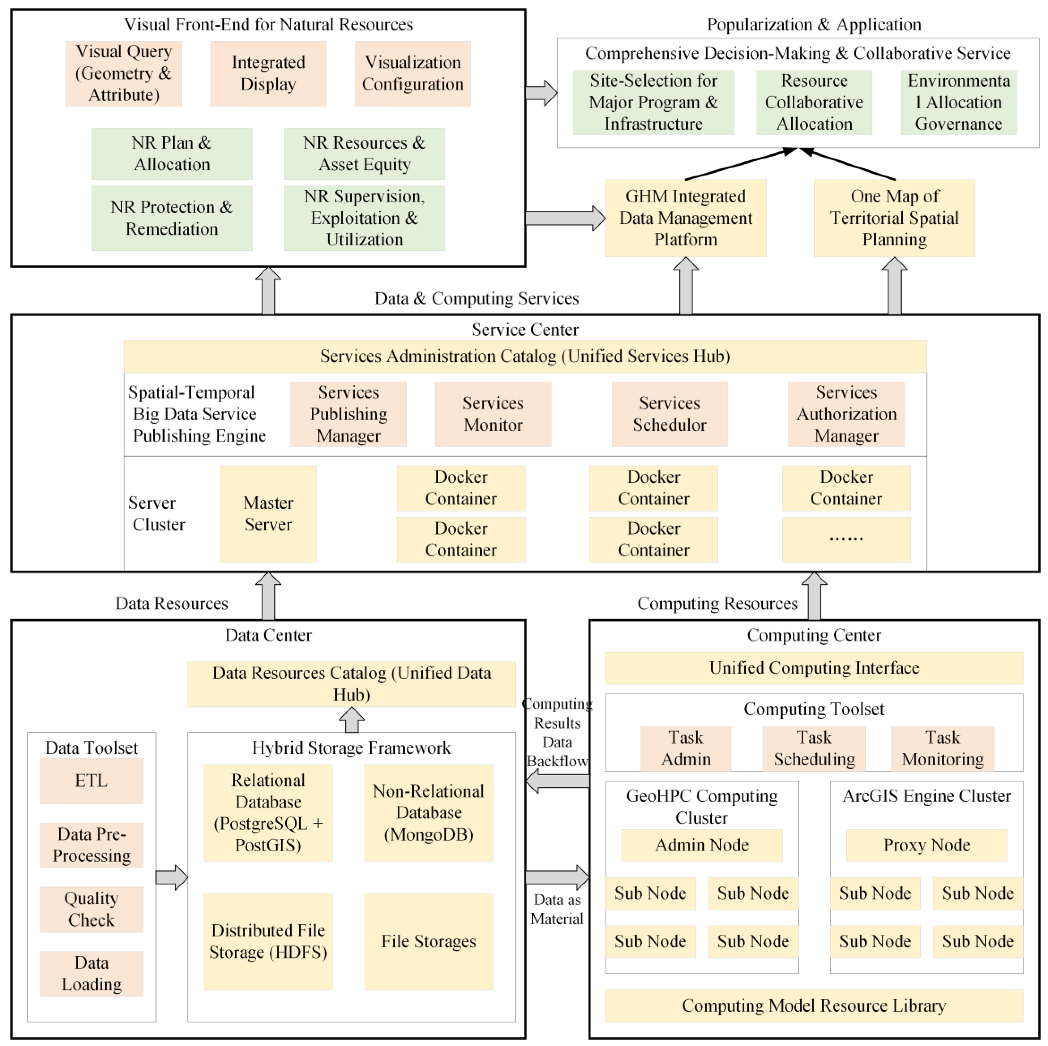
The NRIDB is mainly composed of the Data Center, Computing Center, Service Center and Visual Web Front-End. It is a server-side + web-side GIS designed for the management and service of natural resource big data. The overall architecture is shown in Figure 10.

The Data Center includes a relational database + spatial data engine, nonrelational database (NoSQL), file storage + distributed file storage system, and data toolset, as well as a grouped and a classified data resource catalog based on the data and technology standard specification system. The data resource catalog serves as a unified entry and exit for natural resource and geospatial data. The data toolset includes ETL tools, data pre-processing tools, data quality inspection tools and data importing tools. The relational database + spatial data engine is the core of the Data Center. After all data results underwent pre-processing, quality inspection and other processes, they were imported into each database, the corresponding metadata were generated, and the metadata were imported into the metadata set of the relational database. The Data Center registered the metadata information in the data resource catalog to realize data registration. The data resource catalog established the connection between the metadata and each dataset in the database through the metadata and the unified data access interface to realize integration and unified management.

Based on the hybrid storage framework of the Data Center, the NRIDB realized the centralized management and distributed storage of geospatial and natural resource data. Tabular and vector data were imported and stored in a relational database (PostgreSQL) through a spatial data engine (SDE or PostGIS), raster data such as satellite images were imported and stored in a nonrelational database (MongoDB) after tiling, and data files such as documents were imported and stored in file storage spaces such as HDFS. By integrating the database access interface, file access interface and data service mode into a unified data access interface, various data resources can be shared and accessed to build a Data Center that is consistent and transparent for users.

The Computing Center includes a computing management toolset, GeoHPC cluster, ArcGIS Engine cluster and model repository. The computing management toolset provides computing task scheduling, load balancing, computing node management, computing monitoring and other functions. GeoHPC is a distributed parallel spatial analysis computing engine developed by GeoWay. The GeoHPC cluster consists of multiple GeoHPC computing nodes. In a scene of complex analysis and batch processing scenarios, GeoHPC computing nodes were deployed in real time under the integrated scheduling mechanism, and each node performed spatial analysis and computation concurrently. According to the functions and characteristics of spatial analysis, the computing task scheduling tool automatically adapts and calls the required data, analysis models and computing clusters and automatically divides computing tasks into multiple sub-computing tasks, which are allocated to each computing node for parallel computing. The model repository is used to edit, modify and manage various spatial analysis models.

Taking the ESD spatial analysis in Section 3.4 of this paper as an example, the Computing Center split the intersect analysis computation of land use data and grid data of various scales into multiple computing subtasks to form a computing subtask queue. Each GeoHPC computing node performed parallel spatial stacking analysis according to the computing subtask queue. Finally, the results of each subtask were aggregated to the GeoHPC management node to form the ESEV grid dataset.

The Service Center includes the services administration catalog and server cluster. The server cluster adopts microservice technology and applies the Docker container as the service publishing node to publish various data and spatial analysis computing functions as Web services with standardized interfaces. The server cluster provides the control functions of starting, stopping and updating each service. The services administration catalog is a unified export for Web services. After the data resources in the database and the spatial analysis models in the model repository were published as services and registered in the service administration catalog, they supported various applications of natural resource management and comprehensive decision-making and collaborative services in GHM. The services monitor can check the running status of the services, check whether the service starts normally and dynamically adjust the load balancing and elastic scaling of the server cluster according to the concurrent access pressure of the services.

Different types of data and spatial analysis computing functions were published as different types of Web services. Vector data were published as Web Feature Service (WFS) or Spatial Query Service, or they were made into a thematic map tile and then published as Web Vector Map Service. Image data were published as Web Map Tile Service (WMTS). Spatial analysis models in the model repository were published as Web Processing Service (WPS).

The Visual Web Front-End provides functions such as online visual browsing, query and measurement of natural resources, geospatial data and other source data, and it realizes the integrated display of 2D and 3D data such as vectors, grids, terrain and 3D models. The land use data shown in NRIDB as Figure 11. Combined with text annotations, tables and other forms, the Visual Web Front-End achieved an all-round and intuitive visual display. Through the adaptation of Visual Web Front-End, the visual results can be seamlessly displayed on the Web, large screens and OGC-compatible mobile apps.

Through application promotion, the NRIDB’s data and computing resources will be more effective and useful in the form of Web services. We shared the standardized data services of the Data Center and the spatial analysis computing services of the Computing Center with the Territorial Spatial Planning One Map (TSPOM) and the Land Management Decision Support System. These governmental systems support the management of natural resources in Guangdong Province, such as land resource management, cultivated land protection, territorial spatial planning and control and utilization, and decision support for natural resource development and utilization. The GHM Integrated Data Management Platform (GHM IDMP) for promotion and application supports a series of comprehensive decision-making and collaborative service applications, such as GHM’s collaborative resource allocation and collaborative environmental protection, as shown in Figure 12.

4. Discussion

Within the EFM system, there are considerable controversies and uncertainties about the ESV evaluation of water ecosystems (rivers, wetlands and lakes) and built-up land. Compared with land ecosystems such as cropland and forest, which are relatively “stable”, the water ecosystem uses liquid water with fluidity as the carrier and carries out complex material and energy interactions with other ecosystems and ecological environments. The spatial differences in water ecosystems are far from those in land ecosystems. The benefits and values of water ecosystem services are closely related to watershed runoff, water environment quality, aquatic biological diversity and aquatic biomass, but it is very difficult to obtain these data and conduct quantitative evaluations. Therefore, in the next stage of the study, we can consider introducing a series of water ecosystem indicators and develop an NPP-like indicator to evaluate the service capacity of water ecosystems, which can be used to modify the regional and interannual service functions and their value in the EFM.

In most studies of ESV, built-up land is generally considered a “consumer” of ecosystem services, and its ecosystem service function and the value provided by it are set to 0. In fact, as an important part of the urban compound ecosystem, urban ecological land is composed of small green spaces and waters in the city and plays an important role in protecting the urban ecosystem and improving the urban living environment and the living quality of residents. Changes in the area and spatial distribution of urban ecological land have an important impact on urban ecological security [49,50]. Therefore, the planning and construction of urban ecological land is an important comprehensive approach to solving the contradiction between the urbanization process and natural ecological protection. The various ecological services provided by urban ecological land have both natural and social attributes [10,27]. Urban ecological land not only maintains the stability of the energy flow, material flow and information flow of the ecosystem itself and guarantees the security of the ecological base of urban development but also provides multiple ecosystem services, such as supply, regulation, support and culture for human beings. These are the most direct benefits of ecosystem services enjoyed by urban residents in their daily lives. Therefore, the ecosystem service of ecological land in urbanization areas should not be ignored. For the evaluation of ecosystem service functions of small-scale ecological land in urban areas, it is necessary to introduce comparable quantitative ecological indicators (such as the green index or enhanced vegetation index), combined with more detailed land use data for comparing the difference in ecosystem service capacity between urban green space and land ecosystems, and the quantitative ecological indicators can be used as modification coefficients to evaluate the ecosystem service function and its value provided by urban ecological land in the EFM.

The ESEV is a quantitative indicator representing ecosystem functions and capabilities. To convert ecosystem functions into an ESV of economic value, a monetization unit is needed as a proxy. In Xie’s et al. [24] EFM, this proxy was the standard value volume called the “D value”, which represents the annual economic benefit of a unit area of cropland. However, due to various reasons, such as the lack of modification methods and ecological and social statistics, many researchers directly used the D value of 2010 in China calculated by Xie et al. in the study of different regions and years [25]. This approach ignores the ecosystem service capabilities and socioeconomic regional and interannual differences and variations. Therefore, it is necessary to regionalize and inter-annualize the D value to adapt to the changes in the ecological background and socioeconomic development level in the study area and study year, especially in China’s large cities, with the rapid development of the social economy and urbanization. Based on the EFM of Xie et al., this paper proposes the regionalization and interannual modification methods of the D value. In the method, the structure of the D value modification coefficient section was consistent with Xie’s equation. In terms of the calculation content, the three main crops in the country in Xie’s equation were replaced by the three main crops in the study area, and the interannual modification of the D value was realized by calculating the statistics of different study years. The crop data were compiled from statistics and agricultural assembly documents of China and Guangdong Province, and the calculation maintained the consistency of the reference basis and statistical caliber of Xie’s research. This study used the difference in crop planting structure and its economic benefit in the study area to modify the D value in the study year and study area, and it was an improvement of the EFM; however, the improvement was still insufficient. Although the changes in the economic benefits of the main crops largely reflected the changes in agricultural productivity and socioeconomic development levels, the proportion of economic benefits of crops in the GDP was very low for economically developed regions. For example, Guangdong Province, where the study area is located, is one of the most developed and densely populated regions in China. With rapid socioeconomic development, Guangdong residents have increasingly higher requirements for the ecological environment where they live. Therefore, the demand for ecosystem services in Guangdong is enormous. However, the agricultural economy of Guangdong Province is underdeveloped, the economic benefit of crops per unit area is weak, and the per capita agricultural output value is only 73% of the average national level. In 2016, the total agricultural output value of Guangdong Province accounted for only 4.65% of the GDP, which was lower than the average national level of 8.56%. During 2004–2016, the growth rate of Guangdong’s total agricultural output value (197%) lagged far behind GDP growth (396%) in the same period. Under the background of a large contradiction between ecological supply and demand and weak agricultural benefits in Guangdong Province, the D value modified by the economic benefits of grain crops may be on the low side, which is obviously inconsistent with the economic structure dominated by second and third industries in Guangdong Province. Therefore, it is necessary to introduce the statistics of the GDP, CPI and other indicators of the level of social and economic development into the modification of the D value in EFM in future research [51].

Urbanization profoundly changes the natural landscape of a region. In essence, it is the process of continuous transformation from regional natural ecosystems and agricultural ecosystems to urban ecosystems, which affects or irreversibly changes the structure, process and function of ecosystems [52]. As the increases in forest, grassland, wetland and other ecological lands in the study area cannot compensate for the loss of ecosystem service function caused by the massive expansion of built-up land, this paper presents the net decrease in the total ESEV in the study area.

The ESEV, which is used to characterize the ecosystem service function and capacity in a region, is affected by climate, ecological background quality and various ecological land area changes. The change in the total ESV is based on the change in the total ESEV, which is also affected by the change in the unit ESEV standard value brought about by socioeconomic development. With continuous socioeconomic development, the standard value of a unit’s ESEV continues to rise, making the equivalent of the ecosystem service function increasingly valuable. This phenomenon is embodied in the soaring housing prices of ecologically elegant housing in large cities of China in recent years. Taking Guangzhou as an example, in the past 10 years, due to the superior living environment, the average price increase of eco-housing in the urban fringe was much higher than that in the urban center during the same period.

From 2004 to 2016, the GDP in the study area increased from RMB 47.1 billion to RMB 303.31 billion, with an average growth rate of 16.79%, and the population increased from 1,028,700 to 2,430,500, with an average growth rate of 7.43%. Combined with the results of this study, the ESV accounted for 16.59%, 8.73% and 5.83% of the GDP in 2004, 2010 and 2016, respectively. Over the past decade, with the rapid urbanization process and socioeconomic development, the total GDP and per capita GDP have grown rapidly; however, both the total amount of ESEV and the per capita ESV in the study area have declined significantly. This means that in the current development mode, the ecosystem services and functions have tended to decline, and the ESV added by socioeconomic development has lagged behind GDP growth. This study is consistent with the ESV results of ESV studies in other urban agglomerations [53,54,55].

The differentiated hybrid storage strategy of the Data Center in the NRIDB comprehensively utilizes relational databases, nonrelational databases and distributed file storage for the comprehensive storage of multisource heterogeneous data. Taking the land use data in this paper as an example, the detailed land use patches were usually broken and small, resulting in a very large number of records. The traditional stand-alone GIS software in desktop computers uses.shape data format for storage, which often encounters the problems of slow modification, update, loading and display. When the amount of data is relatively large, the software will fail to load and crash, and it will not perform computing tasks. These problems all affect the efficiency of scientific research. With the support of the geospatial database in the data center, it takes only a few seconds to load, display and update hundreds of thousands of patches in the study area and perform ESD calculations with the grids.

The computing framework of the Computing Center integrates the GeoHPC parallel computing cluster and the ArcGIS Engine computing cluster. Benefiting from the “small data + big data” cluster computing mode of the GeoHPC parallel computing cluster, the ESD calculation results in Section 3.4 in this paper can be completed in just a few seconds, which is dozens of times faster than the traditional spatial analysis computing in stand-alone GIS software on a desktop computer. We are confident that the Computing Center can support Guangdong Province and the GHM to conduct more complex models and deeper, more detailed, and more diverse ecosystem spatial analysis computing.

5. Conclusions

Based on land use change data in southern Guangzhou from 2004 to 2016, we evaluated the ESEV and ESV in the study area, and through spatial grid processing, trend analysis and spatial autocorrelation analysis of the ESEV estimation results, we found that over more than 1 decade, the study area experienced rapid urbanization, the areal extent of built-up land has occupied a large amount of ecological land, and various types of ecological land have been converted to each other. With the land use changes caused by urbanization and other factors, such as changes in the climate and ecological background quality, the total ESEV of the study area increased from 3.32 million in 2004 to 3.37 million in 2010 and decreased to 3.26 million in 2016. Benefitting from the raised standard value volume of the ESEV due to socioeconomic development, the total ESV of the study area increased from 7.81 billion yuan in 2004 to 13.44 billion yuan in 2010 and 17.68 billion yuan in 2016. The socioeconomic development and urbanization process led to a decline in the ESV’s GDP share from 16.59% in 2004 to 5.83% in 2016. The growth of ESV in the study area lagged behind the growth of GDP. The ESD distribution tended to be higher in the east and lower in the west and higher in the south and lower in the north, and the trend lines in the east–west and north–south directions tended to ease gradually. The ESD distribution in the study area had significant spatial autocorrelation, spatial differentiation characteristics, spatial aggregation and scale effects. With the advancement of urbanization, ESD had a significant negative correlation with the research scale and separation distance. The ESD high–high-type areas were concentrated in the eastern and southeastern parts, while the ESD low–low-type areas were concentrated in the central and northern parts.

Socioeconomic development and urbanization complement each other, resulting in the reduction in ecological land and the increasing scarcity of ecosystem service resources. However, socioeconomic development generates higher requirements for the quality of the ecological environment. Therefore, the increasingly sharp contradiction between supply and demand makes the same ecosystem service function increasingly valuable with socioeconomic development. In this paper, it is embodied in the rising D value. The total ESV in the urbanized area remained on an upward trend. China is experiencing a stage of rapid urbanization, and it is foreseeable that development will continue for some time in the future and may trigger an increasing amount of land use changes from natural landscapes to human-dominated landscapes. The ESV evaluation of land use changes realizes the compensation of ecological resources through monetary calculations of ecosystem service functions and benefits to provide an ecological-economic theoretical basis for land resource optimization and sustainable rational urbanization.

The spatial–temporal differentiation of ecosystem service evolution in this paper makes use of the NRIDB’s multisource data aggregation and spatial analysis and computing power by publishing the results as Web services and displaying them in the Visual Web Front-End. This is a practice of applying governmental systems to the research of natural resources and ecosystem services. However, the application of the research results in this paper is relatively shallow. Next, we will promote and apply the research results in this paper through the GHM Integrated Data Management Platform and TSPOM to provide a greater decision-making basis for comprehensive decision making and collaborative service applications, such as the collaborative allocation of natural resources and the collaborative protection of the environment, and seek to provide more abundant support for the development and construction of GHM.