Abstract
Cities continuously evolve and dynamically organize themselves in unbalanced ways and by means of complex processes. Efforts to minimize or solve the problems resulting from spatial inequalities tend to fail when relying on traditional public policies. This work is committed to analyzing the context for implementing public policies and their impacts on the periphery of São Paulo, Brazil. São Paulo is a city characterized by territorial and social heterogeneity and inequality. The materialization of these public policies involves the construction of unified educational centers in peripheral neighborhoods that, in addition to education, offer sports, leisure, and entertainment activities not only to enrolled students but to the wider residents’ community. The adopted methodology was based on cellular automata models driven by remotely sensed images designed to investigate land use and land cover patterns in the surroundings of these educational centers before and after their construction. The achieved results demonstrate that the initial land use and land cover configurations have a great influence on the land use and land cover spatial arrangements after the construction of the educational centers. However, in all the test sites of this research, it was observed that these social infrastructure facilities favored the reproduction of real estate market logic, marked by socially exclusive differentiation and an uneven appreciation of the urban environment.
1. Introduction
According to a recent UN report, urban areas are expected to absorb virtually all the future growth of the world’s population. While 55% of the world’s population lives in urban areas today, this proportion is expected to increase to 68% by 2050 [1]. The urban population is unevenly distributed worldwide, and there is a massive concentration of people in highly urbanized areas, especially in megacities, which are those that shelter at least 10 million people. Nowadays, there are 33 megacities in the world, which accounted for 13% of the world’s urban population in 2018, with Latin America leading the charge in this respect with 18% of its urban population residing in megacities [2].
Although megacities are notable for their size, concentration of economic activities, and active role in the global economy [2], they are usually characterized by severe socioeconomic and spatial inequalities, especially in developing countries. According to [3], a very common situation in most large cities of Latin America is speculation and increased urbanization costs in which the price of land forces the low-income sectors to overcrowd in central areas or to do without basic services in the city surroundings. This argument is supported by [4]. They also stated that, in the urban land market, higher-income groups can outbid lower-income ones for more desirable sites, which are those with access to opportunities and natural amenities, relegating the needy population to squatter settlements or peripheral areas where infrastructure is limited or non-existent and spatial access to jobs or other services is difficult.
In their turn, Namrata Gulati and Tripid Ray [5] affirmed that there exists a relative inequality within the low-income stratum itself. Thus, it is not possible to name the low-income areas of a city with any singular expression, as for instance, periphery, since several types of peripheries coexist in the chaotic dynamics of urban environments. For instance, [6] evaluated the Brazilian ‘favelas’ (squatter settlements) in the light of common variables and concluded that, although they substantially differed from other forms of urban occupation, it was unfeasible to define a universal type of precarious housing comprising all the categories of ‘favelas’.
Some public policy initiatives strive to mitigate these inequalities, including the direct construction of infrastructure. Such policies, however, tend to disregard the peculiarities of peripheral areas. In this sense, within this scope of great heterogeneity in the urban environment, some questions emerge with respect to the implementation of public policies in different regions within a city. Is it possible to have a standard measure with equal effects in different regions of a city? Is the generalization of an urban intervention able to improve downgraded areas of a city to make them comparable to the most-developed areas? Can a given policy solve or otherwise enhance the problem for which it was particularly designed?
This study deals with the impact in terms of the urban land use and land cover dynamics of a public policy implemented in the São Paulo megacity in the southeast of Brazil targeted to meet the demand for social infrastructure. Between the years 2000 and 2010, forty-four units of a multifunctional educational facility named the Unified Educational Center (in Portuguese, “Centro Educacional Unificado”—CEU) were built on sites selected according to a social vulnerability criterion, and nearly all the units were built in peripheral neighborhoods.
This research comprises customized cellular automata-based models especially envisaged for ten pre-selected CEUs and for two transition periods: 2000–2004 and 2004–2010 (respectively, before and after the CEU construction). These models are designed to simulate land use and land cover change, focusing on the local dynamics and interaction patterns of each built unit and its immediate surroundings. The objective of this paper is two-fold: (i) to assess the effectiveness of CEUs in peripheral neighborhoods by analyzing through fieldwork their service provision capacity, as well as their impact on real estate valuation and the derived land use and land cover change processes in the surroundings of these infrastructures before and after their implementation, and to (ii) unravel underlying peculiarities of such processes by means of CA simulation experiments, taking into account the particular characteristics of the concerned peripheral neighborhoods. The contribution of this paper ultimately lies in the very proposal of using CA models and their byproducts to disentangle the implicit effects of public policies on land use and land cover change that cannot be detected by mere analyses of multitemporal satellite images.
2. Public Policies and Cities
Public policy can be generally defined as a system of laws, regulatory measures, courses of action, and funding priorities concerning a given topic (education, health, housing, transportation, etc.) promulgated by a governmental entity or its representatives and conceived to meet social needs [7]. Public policies, especially those related to the construction of social infrastructure, interfere with the spatial organization of cities, mostly bringing about unforeseeable impacts, including unintended land use change processes [8,9,10]. According to [11], any analysis of public policy should make explicit the locational consequences of policy decisions, and it is useful to think of these locational consequences as spatial externalities associated with publicly financed and operated facilities.
In this sense, there are several ways to assess the effectiveness of a public policy, which may not only concern the attainment of its concrete goals, but also the detection of its undesirable side effects. In the particular case of policies designed for social infrastructure implementation, these side effects regard an imbalanced appreciation of land price [12], a decrease in the quality of services offered by such social infrastructure, and also the leakage effect [13], consisting of the migration of activities to another place, therefore causing land use change to occur in other localities. In peripheral urban areas, this effect chiefly refers to the displacement of the original living population in the vicinities of these public facilities to farther areas, a process known as gentrification [14,15], giving rise to the emergence of new informal settlements in legally and environmentally unsuitable sites [6,16].
Along this line of thought, [17] affirms that there is an inherent flaw in public policy nature itself since they are based on predictions and attempts to control a complex and unforeseeable reality. One of the main causes for the failure of such policies, according to the author, lies in the generalization and standardization of actions. For example, the improper generalization of social relationships within the urban domain, mainly in binary categories such as core and periphery or low income and high income, may imply the loss of important nuances that could be explored in the elaboration and implementation of these policies. The focus of the problem then shifts from the question of whether or not a public policy will fail to the issue of unraveling the reasons for and consequences of this failure.
The usage of tools capable of representing and analyzing the complex dynamics of a city increases the possibilities that public policies may have more alternatives, longevity, and flexibility to adapt to the diverse contexts they might encounter [18]. Introducing the flaw in the elaboration of a new public policy allows the attainment of new efficiency standards, as well as lasting results after the policy’s implementation [17].
3. Statement of Purpose and Brief Literature Overview
The urban environment consists of a complex, heterogeneous, and uneven space. It emerges from the materialization of social, political, and economic processes and is characterized by continuous changes and a succession of uses it makes for the Earth’s surface. This is deemed to be the most representative feature of its dynamic status [19].
In this way, land use is key to expressing changes that take place after the implementation of a public policy, including the construction of educational infrastructure, which is the central topic of this article. The methodological framework of this research basically regarded a simulation dynamic model that relied on the paradigm of cellular automata (CA) [20] and could provide trajectories of change that occurred in a given area within a predetermined span of time. In the case of this work, the land use and land cover transitions were simulated as the function of a set of biophysical and infrastructure variables used to calculate the probabilities of land use and land cover change.
Several works worldwide have analyzed urban land use change by means of CA models, taking into account educational infrastructure as one of its drivers. The work of Blecic et al. [21] is an example, in this sense, that developed a model for simulating urban dynamics in the city of Heraklion, Crete, considering a two-fold set of drivers for land use change: (i) socioeconomic aspects, such as social quality, density, and real estate values and (ii) infrastructure variables, such as the traffic system, social infrastructure (e.g., educational facilities), and technical infrastructure. In compliance with this work, [22] conceived a CA model for assessing the effect of land use policies on urban dynamics and concluded that there were strong relationships between the level of infrastructure and services and the urbanization process.
A GIS loosely coupled CA meant to simulate land use change in Lagos, Nigeria, was developed by [23]. Their model, parameterized by a support vector machine (SVM), took into account the closeness to social and technical infrastructure as drivers of changes in land use, and the former one included educational institutions of great size, such as university campuses. Additional works have also strengthened this line of research by means of urban modeling experiments [24,25].
Different from most of the aforementioned studies, which worked either with binary land use classes (urban x non-urban) or with classes of real estate values as in [21], this study dealt with manifold classes of land use and land cover and was meant to investigate land use and land cover patterns in the surroundings of Unified Educational Centers before and after their construction, striving to shed light on the implicit effect of these facilities on the local processes of land use and land cover dynamics as unforeseen spatial externalities. A total of ten CEUs were researched during a ten-year interval defined for the land use and land cover dynamics analysis.
4. Materials and Methods
4.1. Study Area
The public policy devised for the study area, the São Paulo megacity, regarded the implementation of Unified Educational Centers (CEUs) between the years 2000 and 2010. These educational units represented adaptations of former governmental initiatives conceived in Brazil during the 1940s. CEUs not only provide education, but also sports, leisure, and cultural activities to the needy populations of peripheral neighborhoods. They are designed with a fancy architectural style and can cope with the mobility needs of disabled people. Out of the forty-four units built until 2010, a sampling set of ten units (Figure 1) was selected according to the proportion of informal settlements in their surroundings and keeping a minimum of two units per region of São Paulo municipality. The idea was to select representative samples of CEUs (Figure 2) as a function of their frequency of occurrence in each of the four geographic regions of the city: north, south, east, and west. Since the eastern and western regions contain greater quantities of CEUs, we opted for selecting three samples in both areas. In the remaining two regions, namely north and south-southeast, two CEUs were chosen from each one.
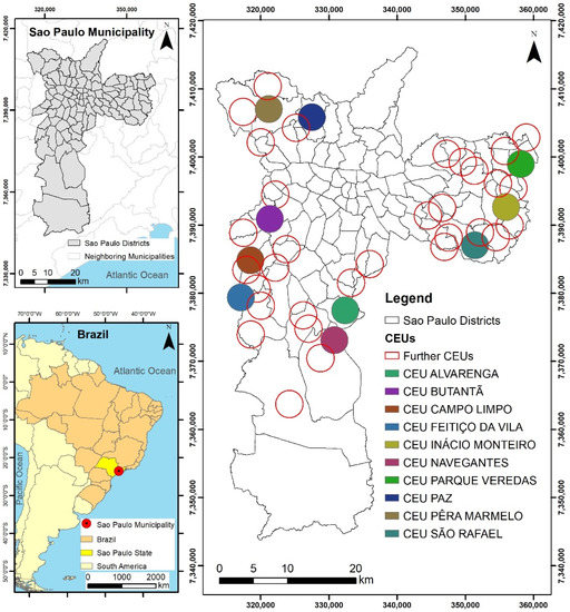
Figure 1.
Study area location.
As to the proportion of informal settlements, we calculated a ratio of the number of pixels classified as informal settlements within each CEU catchment area divided by the area (m2), and the CEUs with the greatest ratio values were selected for analyses.
In Figure 1, it is possible to observe the circular catchment areas of all forty-four CEUs defined by a 2 km radius centered on each unit. The subset of ten CEUs selected for analysis is referred to by the colored circles. The catchment area radius was defined by means of the experimental findings of previous works [26,27] and interviews with the local inhabitants. A methodology was conceived to determine the catchment area radius of the educational facilities, taking into account the level of education provided by the facility, its total built-up area and amount of parking spaces, whether additional services were offered by the facility (sports, leisure, entertainment, etc.), and socioeconomic standard of the residents in the adjacent areas, in addition to the general characteristics of the concerned neighborhood [27]. Considering there were multiple driving variables, the radius of the catchment area may substantially change, but it had a superior threshold associated with the walking distance to be overcome by the target users. The most restrictive option was 1.5 km for pedestrians and approximately 5 km for bikers. In its turn, [26] recommends a catchment area radius of 2 km, which was, in fact, employed in this study.

Figure 2.
Examples of selected CEUs: (a) CEU Paz, (b) CEU Butantã, (c) CEU Navegantes, (d) CEU Pêra Marmelo, (e) CEU Parque Veredas, and (f) CEU Inácio Monteiro. Source: [28].
4.2. Materials and Procedures
The methodology basically consisted of a workflow containing the stages of data pre-processing, parameterization, calibration, simulation, and validation. The simulation process, which was the modeling core stage, departed from an observed initial state of a given system and then reproduced the sequential changes in the system state throughout discrete time steps based on a set of transition rules that were capable of emulating the emerging patterns in a remarkably similar way to how they are seen in reality. Cellular automata are usually the computational framework for simulation models since they easily allow the analysis of the changes’ trajectory and provide a very didactic presentation of results [29]. The following subsections describe each of the above-mentioned modeling stages.
4.2.1. Data Pre-Processing
The input data used in this work, both in terms of land use and land cover maps and explaining variables, are presented in Table 1, which shows their metadata, processing operations, units, and respective sources. All the data used as input for the CA-based simulation models were resampled to remain within 1 m of spatial resolution and in raster format. Initially, the land use and land cover maps were obtained from rectified RGB orthophotos from the years 2000, 2004, and 2010.
The object-based interpretation process regarded twelve land use and land cover classes: Tree Vegetation (green areas with no use), Formal Residential Use, Informal (residential) Settlements, Vacant Plots, Institutional Use, CEU, Paved Roads, Non-paved Roads, Industrial Use, Commerce and Services, Water Dams, and Solid Waste Landfill. Initially, the RGB orthophotos were segmented using multiresolution segmentation [30] in eCognition® [31]. Training samples for the twelve classes were exported to WEKA software 3.8.1 (University of Waikato, Hamilton, New Zealand) for mining in which the C 4.5 algorithm [32] was used. Successive refinements in the training samples were necessary to generate better and more generalizable decision trees. Spectral, texture, geometric, and topological features were used to drive the classification process. The training procedure was crosschecked against fieldwork and consultations with Google Street View and Google Earth [28]. Finally, validation samples were collected, and accuracy metrics were calculated for each CEU catchment area. The obtained Kappa indices ranged from 0.61 to 0.87, and the overall accuracies oscillated between 0.73 and 0.91, which is in compliance with accuracy statistics reported in the literature [33,34,35].
The variables used in the models were subdivided into static and dynamic ones. The former ones remained constant throughout the simulation, and they referred to slope (given in degrees), street network density, and distances to non-canalized water streams and were calculated using Euclidean distance. Variables associated with relief (slope and elevation) and road networks have been commonly used in similar works in the literature [36,37].

Table 1.
Input data description.
Table 1.
Input data description.
| Name | Type | Metadata | Processing Operations | Units | Source |
|---|---|---|---|---|---|
| Land Use and Land Cover in 2000 | Urban landscape map | Orthophoto from 2000 (1 m) | Geobia [38] | - | [39] |
| Land Use and Land Cover in 2004 | Urban landscape map | Orthophoto from 2004 (0.2 m) | Geobia [38] | - | [39] |
| Land Use and Land Cover in 2010 | Urban landscape map | Orthophoto from 2010 (1 m) | Geobia [38] | - | [39] |
| Distance to Land Use and Land Cover Classes | Dynamic variables | Extracted from the Land Use and Land Cover Maps | Euclidean distance to pixels belonging to the land use and land cover classes [40] | meters | - |
| Slope | Static variable | Contour lines with spatial resolutions of 1 m and 5 m | Inverse distance weighting (IDW) interpolation and slope extracted from elevation [41] | degrees | [39] |
| Distance to Non-canalized Water Streams | Static variable | Hydrographic Map—SP | Euclidean distance to pixels belonging to the class Non-canalized Water Streams [40] | meters | [39] |
| Street Network Densities in 2000 and 2004 | Static variable | Road Network Map of Sao Paulo—SP | Number of pixels per square kilometer belonging to the class Streets [42] | pixels/km² | [39] |
The dynamic variables concerned the distance to certain land use and land cover classes and were calculated using Euclidean distance to classes that suffered alterations along the simulation run [40]. For each land use and land cover transition, there was a specific group of dynamic variables, and they were empirically selected during the model calibration. The final procedures of the data pre-processing stage included a crosscheck among all the input data layers to verify their compatibility in terms of the geographic projection system, horizontal datum, bounding box, and spatial resolution.
4.2.2. Parameterization
The parameterization consisted of a double-stage process: (i) firstly, global and annual transition rates were calculated, and (ii) secondly, positive weights of the evidence were calculated using Bayes’ theorem of conditional probability [43].
The global transition rates were obtained through a crosstabulation operation, which essentially referred to basic principles of the Markov chain. The annual transition rates derived from the global transition rates matrix were reckoned based on a method idealized by [44], according to Equation (1):
where M’ is the annual transition matrix; M is the global transition matrix resulting from a crosstabulation map taking into account the initial and the final land use and land cover maps of the given simulation period; H is the eigenvector matrix of M; H−1 is the inverse eigenvector matrix of M; and V is the eigenvalue matrix of M, which is raised to the power 1/n, with n being the number of annual steps. The calculation of the annual transition matrix was possible, provided that the global matrix be ergodic. For a Markov chain to be ergodic, two technical conditions are required of its states and the non-zero transition probabilities: irreducibility and aperiodicity [45]. These annual transition rates were executed at the macro level of the model, accounting for the total amount of land use and land cover transitions in the study area at each time step, and the study area was represented by the entire cellular space, consisting of quadratic grids of around 4000 pixels (columns) × 4000 pixels (rows). These annual rates were responsible for generating the annual land use and land cover simulation maps.
After defining the global transition rates, local transition probabilities needed to be estimated. These probabilities referred to the favorability of cells to change from one land use or land cover to another or, otherwise, to remain in their original state. The weights of evidence method [43] was adopted for this purpose, which relied on the concept of the natural logarithm of odds. Odds provide a measure of the likelihood of a particular outcome, and they are calculated as the ratio of the number of events that produce an outcome to the number that do not, as shown in Equation (2):
The weights of evidence method was implemented in the modeling platform employed in this work—Dinamica EGO [40]. This Bayesian method only deals with categorical variables (or evidence), and hence, variables related to numerical grids (i.e., containing float values such as maps of distance, slope, and density of street networks) had to be discretized by means of slicing operations. Such operations are based on line generalization algorithms and generate ranges with which values of positive weights of evidence () are associated, as calculated as in Equation (3):
where is the probability of variable given the presence of land use and land cover transition , calculated as the number of cells where both and were found divided by the total number of cells where was found; is the probability of variable given the absence of transition , determined by the number of cells where both and were found divided by the total number of cells where was not found. Based on the two equations above, local transition probabilities were then calculated for each cell according to Equation (4):
where is the probability of transition in a cell with coordinates x,y; is the land use and land cover transition; i is the driving variable i selected to explain ; and is the odds of .
A positive weight of evidence indicated the favorability of a certain land use or land cover change to take place in the face of the previous presence of a given evidence. High values of enhanced the probability of an occurring , although there was no causality relation between the transitions and their respective explaining variables. For each observed land use and land cover change of each simulation period, maps of transition probabilities were generated. Any given variable owned a distinct range threshold and, thus, also differentiated values for different land use and land cover transitions, which revealed that the variables’ behaviors changed as a function of the considered transition.
4.2.3. Calibration
Calibration accounted for the iterative procedure of adjusting the variables and parameters by means of a continuous comparison between the real and the simulated scenes to make the simulated scene seem as similar as possible to the real one. Some procedures impacted the transition probabilities maps, while others directly affected the quality of the simulated maps. The first group regarded: (i) eventual changes in the upper and lower limits of the simulation periods, which had, in its turn, consequences on the transition matrix and on the set of explaining variables of the concerned periods; (ii) modifying the parameters for discretizing the continuous variables (either static or dynamic ones) required by the line generalization technique mentioned in Section 4.2.2; (iii) adding or removing explaining variables from the model; and (iv) applying further processing to raw data, such as the generation of a map of street network density based on the road network map by means of Silverman’s algorithm [42].
The second group, which concerned strategies that had an impact on the simulated maps, referred to the setting of internal parameters associated with urban landscape morphology, namely the size, shape, and contiguity of land use and land cover patches. The latter one regarded the share of the two change allocation functions available through the Dinamica EGO platform, also known as transition functions: expander and patcher. Expander accomplished transitions through expansion, and the patcher function, in its turn, executed transitions through diffusion or nucleation. These two functions were complementary, and the sum of their percentages was equal to 1.0 [46].
Additional parameters concerned the patch isometry index (PII) and the size of new land use and land cover patches. PII regarded a numerical value in the interval from 0 to 2, which was multiplied by the probability values of the eight cells belonging to the Moore neighborhood (3 × 3 pixels), before the execution of each change allocation function. The isometry index was responsible for the compactness degree of a patch. Geometrically stable and compact patches implied high values of PII, while dendritic and fragmented patches were obtained by low PII values [47]. This index was set by trial-and-error approaches.
In order to assess the average and variance of patches, given in hectares, as well as the share of the change allocation functions, a spatial SQL was used, relying on maps of individual transitions derived from reclassifications of a crosstabulation map for each study area and simulation period. In a transition from land use and land cover i to land user and land cover j, i was the initial land use and land cover class, and j was the destination one. The individual transition map assigned a null value (0) to pixels of all transitions whose initial land use and land cover class differed from the initial land use and land cover class of the transition under analysis. A value of 1 was assigned to pixels of all the transitions that remained in the destination class of the analyzed transition or to pixels associated with changes to such destination class but departing from an initial land use and land cover class different from the initial land use and land cover class of the considered transition. Finally, a value of 2 was assigned to pixels belonging to the considered transition.
The calibration also comprised tuning procedures aiming to comply with the premise of independence between the variables, which is a basic principle of the probability theory. In this sense, a joint information uncertainty index [43] was used to assess the degree of spatial dependence or spatial association between variables chosen to simulate a certain transition. The joint information uncertainty index (U) belongs to the class of entropy measures and is based on the area crosstabulation matrix between pairs of variables selected to explain the same transition. U was calculated for all the possible pairwise combinations of the variables.
The criterion adopted to verify the variable independence was mostly defined in an assertive way [46]. According to [43], values above 0.5 indicate more association than less. In this way, this value was chosen as a threshold to keep variables in the model. The final variable selection, thus, considered removing spatially dependent variables (U > 0.5), variables with noisy behavior, and those that did not own any explanatory power but coincidently presented a good fit in the model.
4.2.4. Simulation
The simulation of land use and land cover transitions took place after the calibration stage. Two simulation periods were adopted, extending from 2000 to 2004 and from 2004 to 2010, namely before and after the CEU construction. The simulation periods reflected homogeneous circumstances in terms of economic, political, social, institutional, and infrastructural aspects of the analyzed city and consisted of different time durations [48]. Hence, the calibration obtained for one simulation period was by no means transferable to another period, and this happened also because the set of driving variables selected in one simulation period could differ from those chosen in another period, as reported in the literature [49,50]. Very often, the variables may even remain the same or partially the same, but their roles and degree of importance may vary from one period to another.
It is worth reminding that the dynamic distances were recalculated after each time step, and consequently, the transition probability maps were likewise updated after each annual step. All the simulation runs considered annual time steps. The total quantity of cells to experience land use and land cover changes was estimated using the rates of the global transition matrix, which were decomposed in annual rates according to [44].
Expander and patcher were executed by means of random operations in which a random number oscillating from 0 to 255 was compared with the cell probability value, also ranked in 8 bits. If the probability exceeded the random number, then the cell changed its state, or it remained instead in its original state in the case of probability equal to or inferior the random number. The size of a patch, expressed as the total number of its cells, was defined based on a log-normal distribution using the mean and variance patch sizes set by the user. In the face of this random character, although the input data and parameters of the model (i.e., static and dynamic variables, transition rates, positive weights of evidence, percentage of expander and patcher, the patches’ average size and variance, and PII) were kept the same, the morphology of patches in the urban landscape varied from one simulation run to another.
Finally, we must state that the purpose of the simulations was not exclusively the generation of future scenarios. One useful goal of land use and land cover change models is to simulate past and present situations to understand the role of driving variables in such processes of change. In addition, several works in the literature have dealt with CA simulations of past events [46,50,51,52,53,54]. In the particular case of this work, we were committed to analyzing the impact of the CEUs in their vicinities immediately after their construction with respect to land use and land cover change, and hence, we were not interested in assessing their impacts in future time horizons.
4.2.5. Validation
The two simulation periods (before and after the CEU construction) were calibrated in an independent way, and the simulations were run based on the specific calibration obtained for each period. It is worth stating that there is no bias in conducting a validation for a simulation based on a calibration especially produced for a given simulation period since the modeling platform—Dinamica EGO—works with the random allocation of change, as well as the random definition of patch size. Moreover, areas of no change in both real and respective simulated land use and land cover maps were masked out at the validation stage, and these procedures avoided the possibility of tendentiousness in the statistical assessment of similarity between these maps.
For the model statistical validation, the Dinamica EGO platform employed an adaptation of the fuzzy similarity index conceived by [54]. This index establishes similarity metrics between two maps by means of neighborhood windows of different sizes. The central cell class of a window in map 1 was checked against the corresponding window (placed in the same area) in map 2. In a case where the concerned class was also found in the central position within the window in map 2, the metric was set to 1 (100% similar). In a case where the class was found within the window in map 2 but not in the central cell, the similarity metric was penalized as a function of the smaller or greater distance of this cell in relation to the central cell, according to the formula 2−d/2, with d being the unitary distance measured between two cells’ centroids for exponential decay. This was the so-called fuzziness of location. If the constant decay was otherwise adopted, then the similarity remained 1. The similarity dropped to zero in a case where the expected class was not found within the window in map 2 for both types of decay. All the windows were averaged for the whole map, and a comparison was made in both directions (“two-way similarity”), i.e., map 1 in relation to map 2, and map 2 in relation to map 1.
The adapted fuzzy similarity index implemented in Dinamica EGO did not compare map 1 (real final land use and land cover map) with map 2 (simulated final land use and land cover map) as the original index proposed by [55]; rather, two difference maps [56], were generated from the subtraction, on the one hand, between the initial land use and land cover map and the final simulated land use and land cover map and, on the other hand, between the same initial land use and land cover map and the final real land use and land cover map. It is worth mentioning that, not only were the statistics of agreement based on multiresolution contextual windows used, but the resulting morphology of the simulated map was also considered for the model validation.
4.3. Linearity Analysis
After the conclusion of the simulation stage, it was then possible to elaborate a continuous representation of the land use and land cover data based on annual intervals for both simulation periods. For each period, we tried to assess land use and land cover change along the years by means of a continuous line reflecting the shares of land use and land cover areas (ha) in each year, which were extracted from the annual simulation maps. By uniting the two periods’ lines in a single graph, we obtained a linearity assessment for both before and after the CEU implementation. This analysis assumed that the closer the values of the lines’ slopes, the smaller the land use and land cover oscillation between the two periods, as well as that the models could be regarded as linear for the whole time span of the analysis, i.e., from 2000 to 2010. However, if there was a marked slope change between the two lines, we could admit there was a breakpoint or explicit variation in the land use and land cover change patterns before and after the CEU construction [57,58,59].
The land use and land cover classes that did not suffer any transition were discarded from the analysis. The considered angle was the one formed in the inferior side of the lines, and the closer the angle to 180°, the more linear the junction of the lines between the two simulation periods. Values below 180° indicated a deceleration in the respective land use and land cover share, while values above 180° accounted instead for an intensification. It is worth stating that the set of variables and parameters used for the simulations of the analyzed CEUs were unique for each of these ten units. It was possible to identify particular signatures for the analyzed trajectories of land use and land cover shares, i.e., a specific pattern of land use or land cover change after each CEU implementation, which could be interpreted as a local behavior but, in some cases and to a certain extent, could be comparable with the remaining CEUs.
5. Results
5.1. Transition Matrices
As previously stated, transition matrices offer a nonspatial synthetic analysis of land use and land cover change trajectories at a macroscale since they enable the visualization of change directions, i.e., the use of origin and the respective use of destination, among all urban land use and land cover classes. They can be expressed either as global (Tables S1–S10) or annual transition rates along the simulation periods and allow the identification of change fluctuations in particular land use and land cover classes [60].
Table 2 and Table 3 present an assessment of all the types of observed transitions and their respective frequencies in the CEU surroundings for the first and second simulation periods, respectively. When interpreting Table 2, one can notice that the occurrence of transitions from Informal Settlements (coded as 3) to Formal Residential Use (coded as 2) was observed in four out of the ten analyzed CEU units. In the second simulation period, this type of transition took place in eight CEU units, according to Table 3.
Table 2.
Number of CEUs showing different types of transitions in the 1st simulation period: 2000–2004 *.
Table 3.
Number of CEUs showing different types of transitions in the 2nd simulation period: 2004–2010 *.
In Table 2, 62 types of land use and land cover transitions were computed for all the CEU units, while Table 3 amounts to 74 transition types, considering any land use or land cover class within the CEU catchment areas. This increase revealed a greater dynamic of change in the second simulation period.
Table 4 shows the annual transition rates in percentages from Tree Vegetation or Vacant Plots to Informal Settlements for all the CEU units. The rates are presented for the first and second simulation periods. The transition rate was dimensionless. It referred to the division of the total number of pixels that changed from the origin land use or land cover (i.e., the land use or land cover in the initial time of the simulation period) to the destination land use or land cover (i.e., the land use or land cover in the final time of the simulation period) divided by the total number of pixels belonging to the origin land use or land cover of the concerned transition. For the cases that repeated in both periods, a ratio of the second period rate to the first period rate was calculated, indicating either an increase or decrease in the respective rate.
Table 4.
Ratio of the transition rates to Informal Settlements between the two simulation periods.
The ratio values below 1 indicated a reduction in the transition rates to Informal Settlements between the periods, while values above 1 represented the transition rate increase. In this way, it became evident that the rates increased in six out of the nine observed cases. In the Campo Limpo CEU, the annual transition rate from Vacant Plots to Informal Settlements was over eleven times greater in the second simulation period, and in the Parque Veredas CEU, the same type of transition had an annual rate over five times greater in the second period.
In the Butantã and Pêra Marmelo CEUs, Informal Settlements continued to occupy the Vacant Plots, but the rate was smaller in the second period for both units. It is important to observe that, in these two units, the percentage of informal housing in relation to the total area was, respectively, 4.2% and 2.5% in the year 2000, while in 2010 these values changed to 4.3% and 1.9%, respectively. The average share of Informal Settlements within all the CEU catchment areas from 2000 to 2010 was 8.7%.
For cases where the annual transition rate increased in the second period, the a priori percentage of Informal Settlements in relation to the total catchment area was close to or above average with respect to all the CEUs. It was possible to observe that the CEU catchment areas with greater shares of Informal Settlements in the first simulation period tended to maintain or even slightly enhance this pattern after CEU implementation.
5.2. Transition Probabilities
Figure 3 summarizes the behavioral influence of explaining variables for the transition from Informal Settlements to Residential Use in the transition probability map. In the first simulation period (Figure 3a), there existed many patches of squatter settlements with high transition probabilities (reddish colors) for being urbanized, i.e., converted to Formal Residential Use. In the second period (Figure 3b), there was only one patch with a high transition probability, which led us to infer that the CEU implementation may have concentrated the cells prone to undergo such change in areas relatively close to this facility.
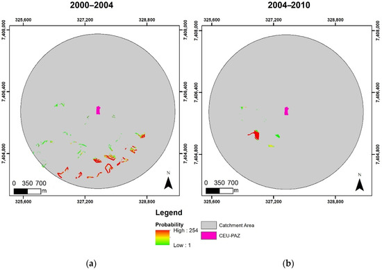
Figure 3.
Transition probability maps from Informal Settlements to Residential Use for the two simulation periods in the Paz CEU from 2000 to 2004 (a) and from 2004 to 2010 (b).
In the comparison provided in Figure 4, one can observe that formal urban expansion showed a peculiar behavior for the two analyzed CEU catchment areas with respect to the probabilities of such a transition. The highest probability values (reddish colors) prevailing in patches with uniform sizes in the Butantã CEU were spread throughout its catchment area. In the Parque Veredas CEU, on the other hand, the patches with the highest probability values and greater areas were mostly found in the farthest distance ranges.
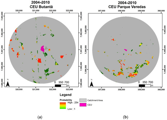
Figure 4.
Transition probability maps from Vacant Plots to Formal Residential Use for the second simulation period in the (a) Butantã CEU and (b) Parque Veredas CEU.
The contexts within which the land use and land cover transitions took place were similar in these two CEUs. Both catchment areas had over 50% of their surface occupied by Formal Residential Use in 2000, which was raised to 52% in the Butantã CEU and 54% in Parque Veredas CEU in 2010. In the Butantã CEU, the annual rate of formal residential expansion was considerably greater in the second simulation period (5%) with respect to the first period (0.3%). From 2000 to 2004, this expansion only involved the transition from Vacant Plots to Residential Use, while the growth in Formal Residential Use in the second simulation period departed from multiple land use and land cover classes, namely Tree Vegetation (0.48%), Vacant Plots (3.8%), Institutional Use (0.13%), and Commerce and Services (0.65%).
In the Parque Veredas CEU, however, the formal residential expansion slightly increased (from 2.8% to 3.3%), associated with an oscillation of near 80% in the rate of the urbanization (regularization) of Informal Settlements in the second period. The conversion from Informal Settlements to Residential Use in the first period reached 0.54%, and this rate was raised to 0.96% in the second period. In both CEU units, there was a decrease in the total area of Informal Settlements.
It is possible to infer that the transition from Vacant Plots to Informal Settlements was entirely dependent on the availability of such unoccupied areas, as in the case of the Paz CEU. In the first simulation period, these plots were more concentrated in the southern sector of the CEU catchment area, while in the second simulation period they were shown to be clustered in a southwestern section closer to the Paz CEU, which acted as an attractor for residential use. The natural trend of such settlements is either their removal or regularization throughout time. In this sense, the Parque Veredas CEU reflected such a trend of residential use formalization, which could be ascribed to the fact that its catchment areas were already characterized by the prevailing occupancy of Formal Residential Use to the detriment of Informal Settlements.
5.3. Linearity Analysis
As formerly exposed, the analysis of the slope angle between the two lines associated with each of the simulation periods enabled the assessment of the impact of CEU implementation in the dynamics of the São Paulo megacity peripheral regions. Figure 5 shows an example of a such an angle for Informal Settlements (coded as 3) from the first simulation period (2000–2004) to the second one (2004–2010) with respect to the Navegantes CEU. Angles below 180° indicated a decreasing share in the respective land use or land cover in the urban landscape of the CEU catchment area.
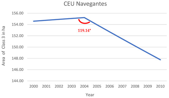
Figure 5.
Slope angle resulting from the joint lines related to the Informal Settlements (Class 3) area in hectares within the catchment area of the Navegantes CEU from 2000 to 2010.
Figure 6 presents examples of signatures associated with trajectories of land use and land cover shares for two CEUs: Navegantes and Paz. The angle shown in Figure 5 regarding the share of Informal Settlements from the first to the second simulation period with regard to the Navegantes CEU is highlighted in Figure 6. Values near 180° accounted for a nearly stationary trend of land use and land cover shares between the two simulation periods. Values above 180° represented an intensification of such land use and land cover, while values below this threshold instead indicated a downshift.
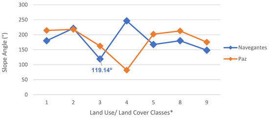
Figure 6.
Comparative graph showing the variations in land use and land cover shares for the Navegantes CEU and Paz CEU as a function of the slope angles. * 1—Tree Vegetation; 2—Residential Use; 3—Informal Settlements; 4—Vacant Plots; 5—Institutional Use; 8—Industrial Use; 9—Commerce and Services.
Table 5 summarizes the lines’ slope angles of each analyzed CEU, and the selected land use and land cover classes are those which presented meaningful variations from one period to another. The land use and land cover classes that did not suffer any transitions were discarded from this analysis. The last line of Table 5 represents the mean angle variations per land use or land cover class for all the CEUs.
Table 5.
Slope angle between the lines of the two simulation periods.
5.4. Simulation
The spatial inequality in the urban tissue organization was also noticeable in the process of the allocation of land use and land cover transitions patches, which emerged in the model simulation operations as a function of the cell transition probabilities. By analyzing all the CEUs with regard to the location of the land use and land cover transitions patches and considering the two simulation periods (Figures S1 and S2, respectively), we could observe that this social infrastructure did not determine the specific location of land use and land cover change, but they interfered with the spatial pattern trend in the emergence of such patches.
Tables S11–S16 present the percentages of the transitions related to formal and informal residential uses in terms of area and the number of patches as a function of four distance ranges for all the analyzed CEUs. Since all the transition patches generated by the model simulations were indexed, it was possible to formulate a synthesis of the main types of change associated with formal and informal residential use within the CEU catchment areas. Initially, Tables S11 and S12 provide percentages of transitions from any kind of land use or land cover to Informal Settlements for all the CEUs with respect to the first and second simulation periods, respectively.
The comparison between Tables S11 and S12 revealed the CEU units in which the locations of patches clusters were modified from one period to another. The Paz CEU, for instance, concentrated patches of transitions to Informal Settlements in the two first distance ranges in the second simulation period. The Navegantes CEU concentrated, otherwise, the expansion of Informal Settlements in the two farthest distance ranges. In this way, it was possible to affirm that these educational facilities redirected the growth of such settlements to specific regions in the surroundings of each CEU according to the a priori spatial organization of such areas. Only three CEU units did not present variations in the informal settlement spatial pattern, namely the Pêra Marmelo, Parque Veredas, and Paz CEUs.
Tables S13 and S14 present the percentages of Informal Settlement removal or urbanization (regularization) in terms of area and the number of patches as a function of four distance ranges for all the analyzed CEUs. These processes accounted for transitions from Informal Settlements to any kind of land use or land cover classes, and they were somehow related to the processes described in the two previous tables. In the Butantã and Pêra Marmelo CEUs, the removal and regularization of Informal Settlements in the second simulation period were concentrated in distant ranges, as opposed to those which presented the expansion of these settlements in the same period. These facts demonstrated that a new spatial division of land use and land cover transitions trends came on the scene after CEU construction.
The percentages of the transitions from any type of land use or land cover class to Formal Residential Use within the CEU catchment areas are shown in Tables S15 and S16 and are arranged as functions of their respective areas and numbers of patches according to four distance ranges.
Tables S15 and S16 provide insights on the spatial organization in the CEU surroundings regarding the expansion of Formal Residential Use. Formal Residential Use patches showed greater permeability among all the distance ranges, or in other words, they were not concentrated as the Informal Settlements were. This phenomenon is supported by [61], who stated that the possibility and the priority for choosing a place to live is directly associated with the level of income. This difference was clearly noticeable between the spatial patterns associated with Formal Residential Use and Informal Settlements.
5.5. Validation
Table 6 presents the minimum values for the fuzzy similarity index, which were calculated for windows of size 5 × 5 pixels with constant decay. Since this index was extracted from a two-way comparison between two difference maps, there was always a minimum and a maximum value, and a tie between these two values was nearly impossible. The minimum index values are presented for both simulation periods for all the CEU units. A threshold of 0.4 was adopted for defining a good fit of the simulation [62].
Table 6.
Values of the fuzzy similarity index (constant decay).
The values presented in Table 6 concern the best simulation produced for each CEU (Figures S1 and S2) out of at least ten runs using the same ideal settings, which were those deemed to produce the best calibration. The simulation selected as best was not only based on the obtained value for the adapted fuzzy similarity index, but also on the morphological agreement between the real and simulated urban landscapes.
Manifold factors impacted the quality of similarity, such as: (i) the amount of change per ranges of the driving variables; (ii) the spatial distribution of change; and (iii) the patch morphology. There were CEUs with vicinities presenting a more stable behavior of land use and land cover change, which tended to increase their fuzzy similarity indices, while there were other CEUs where this behavior was not observed. This fact did not imply that inferences conducted based on the results might be compromised. Moreover, considering that the comparison took into account difference maps that masked out areas of no change, any value for the fuzzy similarity index above the adopted threshold was regarded as acceptable.
6. Discussion
The main changes involved Formal Residential Use, Vacant Plots, and Informal Settlements, which seemed to indicate a close relationship between formal and informal horizontal residential growth in the periphery of the São Paulo megacity [63,64].
There was, in fact, a considerable increase in transitions from Informal Settlements to Formal Residential Use and Vacant Plots after CEU construction, which demonstrated an intensification in squatter settlement urbanization (formalization) or of their removal. Nevertheless, the transition frequency from Tree Vegetation or Vacant Plots to Informal Settlements remained the same, which typically characterizes peripheral urban occupation. Another change worthy of notice was the increase in the transitions from Vacant Plots to Residential Use, indicating an expansion trend of the formal city in these areas during the second simulation period. All these changes revealed that these educational facilities promoted real estate appreciation and a consequent regularization of Informal Settlements or, otherwise, the displacement of precarious housing inhabitants from the CEU surroundings to farther areas.
When analyzing the role of the explaining variables, it was possible to conclude that there was no standard behavior concerning their roles in the observed transitions. It was precisely the occupation context of each CEU catchment area and its physical site characteristics that determined the impact of a given variable on the land use and land cover change. In the case of Water Dams, which was solely found in the Navegantes CEU, it was observed that the highest weight values were seen in the closest distance ranges for the conversions to Residential Use, while in the transitions to Informal Settlements, the highest weights were found in the farthest distances from the dam.
The variable of Street Network Density likewise showed a non-uniform behavior. The transition from Tree Vegetation to Informal Settlements was usually associated with low values of Street Network Density in both periods of the analysis. However, in the transition from Tree Vegetation to Residential Use, the highest weights were observed in the medium and high values of Street Network Density. This indicated that Formal Residential Useexpansion took place in consolidated urban areas, while Informal Settlements were found in precarious sites with limited infrastructure. The conversion from Vacant Plots to Informal Settlements in the Campo Limpo and Paz CEUs, for instance, corroborated this statement since it was associated with high values of slope, such as steep hillsides.
The comparison of the transition probabilities from Vacant Plots to Informal Settlements between the two periods indicated that changes in the spatial pattern of such a transition as a function of the explaining variables occurred in several CEU units. In the Paz CEU, for instance, located in the northern region of the city, it was possible to observe a connection of this transition in areas close to this CEU, i.e., the probability of this land use and land cover change to occur in this CEU vicinity was considerably greater.
In a general way, considering all the driving variables and respective ranges in all the CEUs, as previously explained, there was no common behavior regarding the influence of such variables on the observed land use and land cover transitions. In each CEU catchment area, the set of intervening variables had a local explanatory power and could by no means be generalized. Nevertheless, the CEUs showed a catalyzing effect for residential expansion.
The CEU implementation set a new real estate valuation dynamic in their surroundings. Transects or patches of appreciated areas probably arose due to their proximity to social infrastructure. These facts can explain the changes in the annual rates of Informal Settlement removal and of residential expansion associated with both formal and informal residential use, as well as fluctuations in the behavior of the areas owning the greatest probabilities for these land use and land cover transitions as a function of the CEU locations.
The impact of CEUs in land use and land cover transitions was reflected in the maps of transition probabilities, which were built based on the driving variables’ positive weights of evidence (). In order to assess the real role of driving variables, including the CEUs themselves, in terms of location, patch geometry, and values of transition probabilities, it was mandatory to go through the whole process of parameterization, calibration, and simulation. It is worth reminding that this was not linear since, after the obtainment of the first simulations, new loops of parameterization, calibration, and simulation procedures commonly take place to render the simulated scene as close as possible to the real scene. These procedures included the insertion or removal of variables, subjecting some variables to new forms of spatial treatment (kernel analysis, linear elements density assessment, etc.), changing the parameters for the discretization of continuous variables, and adjusting the internal parameters of Dinamica EGO (e.g., mean size and size variance of patches, patch isometry index, percentage of the change allocation functions—expander and patcher).
In sum, the value of , which expressed the real contribution of each driving variable for the land use and land cover transitions, only became definite after all the successive iterations of the modeling process, including cycles of parameterization, calibration, and simulation. This information was impossible to be obtained from mere analyses of multitemporal satellite images, such as the generation of crosstabulation matrices and maps, or even an independent weights of evidence analysis detached from the modeling stages. This justified the use of CA modeling to assess undesirable side-effects associated with the implementation of public facilities, such as real estate appreciation processes and the leakage effect, relying on a closer focus on the positioning, morphology, and intensity of transition probability patches. As stated by [11], in large, complex, urban systems, such externalities are particularly critical.
Another finding was the correspondence between the spatial pattern of the new Formal Residential Use patches and the distance ranges containing removals or regularizations of Informal Settlements. This fact could be explained by land appreciation theories and essays targeted to informal markets, which approach such alternate forms of urban land occupation [65,66,67]. The São Rafael and Feitiço da Vila CEUs typically illustrated this finding (see Tables S14 and S16), revealing the predominance of Informal Settlement removal and the occupation of Formal Residential Use in the intermediate distance ranges.
In brief, the results analysis showed us that the implementation of CEUs triggered a cyclic reproduction of real estate market logic, boosting an uneven land price appreciation, and the consequent removal of Informal Settlements or their formalization, commonly ousting their inhabitants to farther areas. This educational policy, meant to assure democratic access to culture, sport, and leisure, actually led to an increase in living costs and unfavorable changes in the priority of residential choice and the intraurban residential mobility of the affected local residents.
The left column of Figure 7 presents a brief timeline of Google Earth images showing the dynamics of land use and land cover change in the vicinities of the Paz CEU in 2008, 2012, and 2021 surrounded by formal (to the west) and Informal Settlements (to the east) placed in a critical neighborhood. We noticed that the locals, in a struggle for living space, invaded the skate track site, which was barely discernible in the latest image, since the clustering of shanties practically “devoured” the track (Figure 8), jeopardizing the service provision capacity of this CEU. On the other hand, the right column of Figure 7 displays the case of the successful Butantã CEU, located amid formal low- and middle-class neighborhoods. Its green areas are intact, and its installations, in good maintenance conditions, have been sheltering since 2013 a tuition-free university targeted to the local community, widening its service provision scope. Therefore, we ought to recognize that the success in the implementation of such an educational public policy in the periphery of the São Paulo megacity was essentially context dependent. The pre-existing conditions were, hence, decisive for the success or failure of the CEU construction initiatives, and their impacts on the vicinities may either improve or worsen the residents’ living conditions.
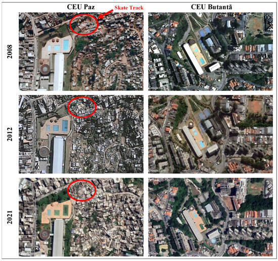
Figure 7.
Comparative images of the Paz CEU and Butantã CEU vicinities in 2008, 2012, and 2021. Source: [28].
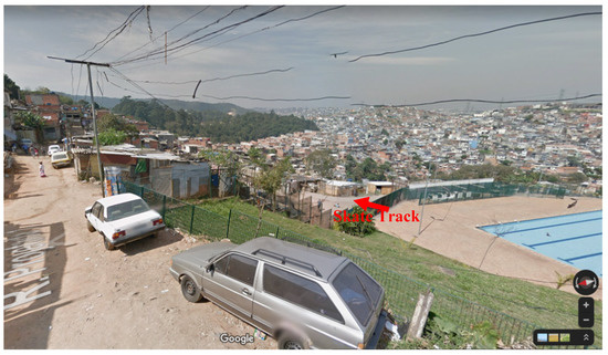
Figure 8.
View of the Paz CEU skate track “stifled” by a squatter settlement. Source: [28].
This demonstrated that the standardization of a public policy is not able to tackle the complex heterogeneity that exists in a city. The CEU policy design hindered the flexibilization and development of solutions that could move far beyond the intended aesthetical and political communication purposes. Some CEU units were implemented in places with no solid waste collection, no sewage system, and hazardous geotechnical conditions, and they prioritized cultural, sports, and leisure services for part of the population still facing basic housing problems [68], in addition to underemployment and unemployment.
It is plausible to think that some CEUs could have redesigned their scope of programmatic activities, granting priority to capacity building (including both training and mentorships), targeted to prepare the locals for job opportunities. Authors such as [69] argue that pure investments in education may keep governments in developing countries in a poverty trap instead of strengthening the link between economic growth and poverty reduction. This initiative undertaken in the São Paulo megacity warns us that public policies, and educational policies in particular, ought to cope with their target audience’s hierarchy of demands and seriously take into account its socioeconomic conditions and the urban context in which the people live.
7. Conclusions
Based on the results obtained in this work, we could acknowledge that the comparisons between the two simulation periods, before and after CEU construction, revealed systematic variations in the model global transition rates. The adopted calibration parameters yielded patches with great variability in space and time, and their main modifications were generated as a function of their distance to the CEUs, the pre-existing spatial context in the catchment area, and the concerned simulation period.
The CA models were demonstrated to be useful for identifying the real role of driving variables for land use and land cover change. Considering that the iterative procedures of the modeling process refined the way such variables were defined and interpreted, the final values of allowed the analyses of the location, morphology, and intensity of the transition probability patches, unraveling the locational consequences of policy decisions, such as publicly operated infrastructure, as in the case of this study. As directions for future work, we intend to extend this methodological approach to assess the impact of further social infrastructure facilities (health-related services, housing, sports facilities, etc.) on land use change processes, exploring artificial intelligence methods, such as deep learning, both for satellite image classification and cellular automata model parameterization.
The transition probability maps generated relying on the values showed that the CEUs generally acted as attractors of both formal and informal residential use but with some peculiarities associated with the spatial characteristics of the concerned catchment areas. Since these facilities promoted an appreciation in land price in their surroundings, the natural trend of Informal Settlements was either their removal or regularization throughout time.
The spatial and temporal variations of land use and land cover change observed at a local scale in the surroundings of each CEU owned direct relationships with the territorial arrangement found before the construction of such educational facilities. This confirmed that the standardization of a public policy is not able to tackle the complex heterogeneity that exists in a city. The CEUs implemented amid residents with better socioeconomic conditions were shown to be successful, as in the case of the Butantã CEU, which even widened its scope of originally envisaged activities and operated under ideal maintenance conditions. On the other hand, the Paz CEU, located in a low-income neighborhood and surrounded by residents living in precarious conditions, had part of its installations illegally occupied by informal housing and significantly reduced its service provision capacity. Furthermore, the unforeseen effects of land use and land cover change resulting from the Paz CEU implementation led to a wider reach of leakage effect in which the population originally living in its surroundings, expelled by the force of land price appreciation, invaded the Cantareira State Park buffer zone, located on the northern fringe of the city, bringing about undesirable environmental consequences.
These findings provided evidence that successful policy initiatives ought to cope with their flaws, anticipating their unintentional externalities and incorporating such flaws in their elaboration. Policies must ultimately avoid generalizations, acquire a deep understanding of the needs of the people for which they are designed, and above all, must not be conceived separately, i.e., dissociated from related policies, for they run the risk of failing to achieve their goals. The CEU policy should, in fact, have been associated with professional development, job creation, social housing, sanitation, and similar policies.
Supplementary Materials
The following supporting information can be downloaded at: https://www.mdpi.com/article/10.3390/land11060922/s1, Table S1: CEU Alvarenga global transition rates for the 1st and 2nd simulation periods; Table S2: CEU Butantã global transition rates for the 1st and 2nd simulation periods; Table S3: CEU Campo Limpo global transition rates for the 1st and 2nd simulation periods; Table S4: CEU Feitiço da Vila global transition rates for the 1st and 2nd simulation periods; Table S5: CEU Inácio Monteiro global transition rates for the 1st and 2nd simulation periods; Table S6: CEU Navegantes global transition rates for the 1st and 2nd simulation periods; Table S7: CEU Parque Veredas global transition rates for the 1st and 2nd simulation periods; Table S8: CEU Paz global transition rates for the 1st and 2nd simulation periods; Table S9: CEU Pêra Marmelo global transition rates for the 1st and 2nd simulation periods; Table S10: CEU São Rafael global transition rates for the 1st and 2nd simulation periods; Figure S1. Simulated and observed land use and land cover maps for the year 2004; Figure S2. Simulated and observed land use and land cover maps for the year 2010; Table S11: Percentage of transitions to informal settlements in the 1st simulation period for all CEUs; Table S12: Percentage of transitions to informal settlements in the 2nd simulation period for all CEUs; Table S13: Percentage of informal settlement removal or urbanization (regularization) in the 1st simulation period for all CEUs; Table S14: Percentage of informal settlement removal or urbanization (regularization) in the 2nd simulation period for all CEUs; Table S15: Percentage of transitions to formal residential use in the 1st simulation period for all CEUs; Table S16: Percentage of transitions to formal residential use in the 2nd simulation period for all CEUs.
Author Contributions
Conceptualization, P.B.R.C., C.M.d.A. and A.P.d.Q.; methodology, P.B.R.C. and C.M.d.A.; software, P.B.R.C.; validation, P.B.R.C. and C.M.d.A.; formal analysis, P.B.R.C., C.M.d.A. and A.P.d.Q.; investigation, P.B.R.C., C.M.d.A. and A.P.d.Q.; data curation, P.B.R.C.; writing—original draft preparation, P.B.R.C., C.M.d.A. and A.P.d.Q.; visualization, P.B.R.C., C.M.d.A. and A.P.d.Q.; supervision, C.M.d.A. and A.P.d.Q. All authors have read and agreed to the published version of the manuscript.
Funding
This research had the support of the Brazilian National Council for Scientific and Technological Development CNPq, through grants N° 311324/2021-5 and 307725/2020-0, and the CAPES Foundation, through grant N° 1563053/2015-2018.
Conflicts of Interest
The authors declare no conflict of interest.
References
- United Nations. World Urbanization Prospects; Department of Economic and Social Affairs: New York, NY, USA, 2019; Available online: https://population.un.org/wpp/Publications/Files/WPP2019_Highlights.pdf (accessed on 22 August 2020).
- United Nations. World Cities Report—The Value of Sustainable Urbanization; United Nations Human Settlements Programme—UN-Habitat: Nairobi, Kenya, 2020; Available online: https://unhabitat.org/sites/default/files/2020/10/wcr_2020_report.pdf (accessed on 22 September 2021).
- Geisse, G.; Sabatini, D. Urban land policy problems in Latin America. Habitat Int. 1980, 4, 671–690. [Google Scholar] [CrossRef]
- Vetter, D.M.; Rzezinski, H.C. The Brazilian case: Land policy for whom? Habitat Int. 1980, 4, 485–498. [Google Scholar] [CrossRef]
- Gulati, N.; Ray, T. Inequality, neighbourhoods and welfare of the poor. J. Dev. Econ. 2016, 122, 214–228. [Google Scholar] [CrossRef][Green Version]
- Brueckner, J.K.; Mation, L.; Nadalin, V.G. Slums in Brazil: Where are they located, who lives in them, and do they ‘squeeze’the formal housing market? J. Hous. Econ. 2019, 44, 48–60. [Google Scholar] [CrossRef]
- Kilpatrick, D.G.; Ross, M.E. Torture and human rights violations. In Mental Health Consequences of Torture; Gerrity, E., Keane, T.M., Tuma, F., Eds.; Kluwer Publishing: New York, NY, USA, 2001; pp. 317–331. [Google Scholar] [CrossRef]
- Boyle, M.; Hall, T.; Lin, S.; Sidaway, J.D.; van Meeteren, M. Public Policy and Geography, 2nd ed.; Elsevier: Amsterdam, The Netherlands, 2020. [Google Scholar]
- Elacqua, G. The impact of school choice and public policy on segregation: Evidence from Chile. Int. J. Educ. Dev. 2012, 32, 444–453. [Google Scholar] [CrossRef]
- Martin, P. Public policies, regional inequalities and growth. J. Public Econ. 1999, 73, 85–105. [Google Scholar] [CrossRef]
- Mercer, J.; Barnett, R. Spatial modifications to models of the urban policy process. Policy Stud. J. 1975, 3, 320–325. [Google Scholar] [CrossRef]
- Carruthers, J.I.; Ulfarsson, G.F. Urban sprawl and the cost of public services. Environ. Plan. B Plan. Des. 2003, 30, 503–522. [Google Scholar] [CrossRef]
- Lambin, E.F.; Meyfroidt, P. Global land use change, economic globalization, and the looming land scarcity. Proc. Natl. Acad. Sci. USA 2011, 108, 3464–3472. [Google Scholar] [CrossRef]
- Walks, R.A.; Maaranen, R. The Timing, Patterning, & Forms of Gentrification & Neighbourhood Upgrading in Montreal, Toronto, & Vancouver, 1961 to 2001; Centre for Urban and Community Studies, Cities Centre, University of Toronto: Toronto, ON, Canada, 2008. [Google Scholar]
- Zuk, M.; Bierbaum, A.H.; Chapple, K.; Gorska, K.; Loukaitou-Sideris, A. Gentrification, displacement, and the role of public investment. J. Plan. Lit. 2018, 33, 31–44. [Google Scholar] [CrossRef]
- Duren, N.R.L. Why there? Developers’ rationale for building social housing in the urban periphery in Latin America. Cities 2018, 72, 411–420. [Google Scholar] [CrossRef]
- Mueller, B. Why public policies fail: Policymaking under complexity. EconomiA 2020, 21, 311–323. [Google Scholar] [CrossRef]
- Agyemang, F.S.; Silva, E. Simulating the urban growth of a predominantly informal Ghanaian city-region with a cellular automata model: Implications for urban planning and policy. Appl. Geogr. 2019, 105, 15–24. [Google Scholar] [CrossRef]
- Batty, M. Fifty years of urban modeling: Macro-statics to micro-dynamics. In The Dynamics of Complex Urban Systems; Albeverio, S., Andrey, D., Giordano, P., Vancheri, A., Eds.; Physica-Verlag: Heidelberg, Germany, 2008; pp. 1–20. [Google Scholar]
- Wolfram, S. Statistical mechanics of cellular automata. Rev. Mod. Phys. 1983, 55, 601. [Google Scholar] [CrossRef]
- Blecic, I.; Cecchini, A.; Prastacos, P.; Trunfio, G.A.; Verigos, E. Modelling urban dynamics with cellular automata: A model of the city of Heraclion. In Proceedings of 7th AGILE Conference on Geographic Information Science; AGILE: Heraklion, Greece, 2004; pp. 313–323. [Google Scholar]
- Kumar, U.; Mukhopadhyay, C.; Ramachandra, T.V. Cellular automata and Genetic Algorithms based urban growth visualization for appropriate land use policies. In Proceedings of the The Fourth Annual International Conference on Public Policy and Management; Centre for Public Policy, Indian Institute of Management (IIMB): Bangalore, India, 2009. [Google Scholar]
- Okwuashi, O.; McConchie, J.; Nwilo, P.; Isong, M.; Eyoh, A.; Nwanekezie, O.; Eyo, E.; Ekpo, A.D. Predicting future land use change using support vector machine based GIS cellular automata: A case of Lagos, Nigeria. J. Sustain. Dev. 2012, 5, 132–139. [Google Scholar] [CrossRef]
- Wahyudi, A.; Liu, Y. Cellular automata for urban growth modelling: A review on factors defining transition rules. Int. Rev. Spat. Plan. Sustain. Dev. 2016, 4, 60–75. [Google Scholar] [CrossRef]
- Zhao, C.; Fang, D.A. Conceptual Model for Urban Interdependent Technical and Social Infrastructure Systems. In Proceedings of the Construction Research Congress 2018, New Orleans, LA, USA, 2–4 April 2018; pp. 722–731. [Google Scholar] [CrossRef]
- Melendez, A. Park-Schools are educational alternatives and urban references. Rev. Proj. Des. 2003, 284, 62–68. [Google Scholar]
- Neves, F.H. The planning of urban community education facilities: Some reflections. Cad. Metrópole 2015, 17, 503–516. [Google Scholar] [CrossRef][Green Version]
- Google Inc. Google Earth Maps/Google Street View. Available online: https://www.google.com.br/intl/pt-BR/earth/ (accessed on 19 April 2021).
- Couclelis, H. Cellular worlds: A framework for modeling micro-macro dynamics. Environ. Plan. A 1985, 17, 585–596. [Google Scholar] [CrossRef]
- Baatz, M.; Schäpe, A. Multiresolution Segmentation—An optimization approach for high quality multi-scale image segmentation. In Angewandte Geographische Informationsverarbeitung XII; Strobl, J., Blaschke, T., Griesebner, G., Eds.; Wichmann: Heidelberg, Germany, 2000; pp. 12–23. [Google Scholar]
- eCognition. eCognition Developer 9.3.1: User Guide; Trimble: Sunnyvale, CA, USA, 2018. [Google Scholar]
- Quinlan, J.R. Programs for Machine Learning; Elsevier: Amsterdam, The Netherlands, 2014. [Google Scholar]
- Taherzadeh, E.; Shafri, H.Z. Using hyperspectral remote sensing data in urban mapping over Kuala Lumpur. In Proceedings of the 2011 Joint Urban Remote Sensing Event, Munich, Germany, 11–13 April 2011; pp. 405–408. [Google Scholar] [CrossRef]
- Longbotham, N.; Chaapel, C.; Bleiler, L.; Padwick, C.; Emery, W.J.; Pacifici, F. Very high resolution multiangle urban classification analysis. IEEE Trans. Geosci. Remote Sens. 2011, 50, 1155–1170. [Google Scholar] [CrossRef]
- Khodadadzadeh, M.; Li, J.; Plaza, A.; Bioucas-Dias, J.M. Hyperspectral image classification based on union of subspaces. In Proceedings of the 2015 Joint Urban Remote Sensing Event (JURSE), Lausanne, Switzerland, 30 March–1 April 2015; pp. 1–4. [Google Scholar] [CrossRef]
- Pan, X.; Wang, Z.; Huang, M.; Liu, Z. Improving an Urban Cellular Automata Model Based on Auto-Calibrated and Trend-Adjusted Neighborhood. Land 2021, 10, 688. [Google Scholar] [CrossRef]
- Zhao, L.; Liu, X.; Xu, X.; Liu, C.; Chen, K. Three-Dimensional Simulation Model for Synergistically Simulating Urban Horizontal Expansion and Vertical Growth. Remote Sens. 2022, 14, 1503. [Google Scholar] [CrossRef]
- Kohli, D.; Sliuzas, R.; Stein, A. Urban slum detection using texture and spatial metrics derived from satellite imagery. J. Spat. Sci. 2016, 61, 405–426. [Google Scholar] [CrossRef]
- PMSP—Prefeitura Municipal de São Paulo. Digital Map of the São Paulo City: Geosampa. 2016. Available online: https://geosampa.prefeitura.sp.gov.br/PaginasPublicas/_SBC.aspx (accessed on 12 April 2016).
- Rodrigues, H.O.; Soares-Filho, B.S.; Costa, W.D.S. Dinamica EGO, a platform for environmental systems modeling. In Proceedings of the XIII Brazilian Symposium on Remote Sensing; National Institute for Space Research—INPE: Florianopolis, Brazil; pp. 3089–3096. Available online: http://marte.dpi.inpe.br/col/dpi.inpe.br/sbsr@80/2006/11.06.17.59/doc/3089-3096.pdf (accessed on 20 March 2021).
- Watson, D.F. A refinement of inverse distance weighted interpolation. Geoprocessing 1985, 2, 315–327. [Google Scholar]
- Silverman, B.W. Density Estimation for Statistics and Data Analysis; CRC Press: London, UK, 1986. [Google Scholar]
- Bonham-Carter, G.F. Geographic Information Systems for Geoscientists-Modeling with GIS: Computer Methods in the Geoscientists; Pergamon Press: Oxford, UK, 1994; Volume 13, p. 398. [Google Scholar]
- Bell, E.J.; Hinojosa, R.C. Markov analysis of land use change: Continuous time and stationary processes. Socio-Econ. Plan. Sci. 1977, 11, 13–17. [Google Scholar] [CrossRef]
- Manning, C.D.; Raghavan, P.; Schutze, H. Introduction to Information Retrieval; Cambridge University Press: Cambridge, UK, 2008; p. 482. [Google Scholar]
- Almeida, C.M.; Batty, M.; Monteiro, A.M.V.; Câmara, G.; Soares-Filho, B.S.; Cerqueira, G.C.; Pennachin, C.L. Stochastic cellular automata modeling of urban land use dynamics: Empirical development and estimation. Comput. Environ. Urban Syst. 2003, 27, 481–509. [Google Scholar] [CrossRef]
- Ximenes, A.C.; Almeida, C.M.; Amaral, S.; Escada, M.I.S.; Aguiar, A.P.D. Dynamic deforestation modeling in the Amazon. Bull. Geod. Sci. 2008, 14, 370–391. Available online: https://revistas.ufpr.br/bcg/article/view/12564 (accessed on 16 May 2022).
- Aguejdad, R. The influence of the calibration interval on simulating non-stationary urban growth dynamic using CA-Markov model. Remote Sens. 2021, 13, 468. [Google Scholar] [CrossRef]
- Teixeira, A.M.G.; Soares-Filho, B.S.; Freitas, S.R.; Metzger, J.P. Modeling landscape dynamics in an Atlantic Rainforest region: Implications for conservation. For. Ecol. Manag. 2009, 257, 1219–1230. [Google Scholar] [CrossRef]
- Yang, J.; Gong, J.; Tang, W.; Liu, C. Patch-based cellular automata model of urban growth simulation: Integrating feedback between quantitative composition and spatial configuration. Comput. Environ. Urban Syst. 2020, 79, 101402. [Google Scholar] [CrossRef]
- Campos, P.B.R.; Almeida, C.M.; Queiroz, A.P. Educational infrastructure and its impact on urban land use change in a peri-urban area: A cellular-automata based approach. Land Use Policy 2018, 79, 774–788. [Google Scholar] [CrossRef]
- Roodposhti, M.S.; Hewitt, R.J.; Bryan, B.A. Towards automatic calibration of neighbourhood influence in cellular automata land-use models. Comput. Environ. Urban Syst. 2020, 79, 101416. [Google Scholar] [CrossRef]
- Silva, C.A.; Giannotti, M.A.; Almeida, C.M. Dynamic modeling to support an integrated analysis among land use change, accessibility and gentrification. Land Use Policy 2020, 99, 104992. [Google Scholar] [CrossRef]
- Mustafa, A.; Ebaid, A.; Omrani, H.; McPhearson, T. A multi-objective Markov Chain Monte Carlo cellular automata model: Simulating multi-density urban expansion in NYC. Comput. Environ. Urban Syst. 2021, 87, 101602. [Google Scholar] [CrossRef]
- Hagen, A. Fuzzy set approach to assessing similarity of categorical maps. Int. J. Geogr. Inf. Sci. 2003, 17, 235–249. [Google Scholar] [CrossRef]
- Almeida, C.D.; Gleriani, J.M.; Castejon, E.F.; Soares-Filho, B.S. Using neural networks and cellular automata for modelling intra-urban land-use dynamics. Int. J. Geogr. Inf. Sci. 2008, 22, 943–963. [Google Scholar] [CrossRef]
- Caruso, G.; Peeters, D.; Cavailhès, J.; Rounsevell, M. Spatial configurations in a periurban city. A cellular automata-based microeconomic model. Reg. Sci. Urban Econ. 2007, 37, 542–567. [Google Scholar] [CrossRef]
- Chow, G.C. Tests of equality between sets of coefficients in two linear regressions. Econom. J. Econom. Soc. 1960, 28, 591–605. [Google Scholar] [CrossRef]
- Rey, S.J.; Montouri, B.D. US regional income convergence: A spatial econometric perspective. Reg. Stud. 2010, 33, 143–156. [Google Scholar] [CrossRef]
- Joint Research Centre—JRC; European Commission—Institute for Remote Sensing Applications; European Space Agency—Earthnet Programme Office—ESA-ESRIN. Modelling Deforestation Processes—A Review; ECSC-ECEAEC: Luxembourg, 1994. [Google Scholar]
- Werna, E. Urban management and intra-urban differentials in Sao Paulo. Habitat Int. 1995, 19, 123–138. [Google Scholar] [CrossRef]
- Macedo, R.C.; Almeida, C.M.; Santos, J.R.; Rudorff, B.F. Spatial dynamic modeling of land cover and land use change associated with the sugarcane expansion. Bull. Geod. Sci. 2013, 19, 313–337. [Google Scholar] [CrossRef]
- Few, R.; Gouveia, N.; Mathee, A.; Harpham, T.; Cohn, A.; Swart, A.; Coulson, N. Informal sub-division of residential and commercial buildings in Sao Paulo and Johannesburg: Living conditions and policy implications. Habitat Int. 2004, 28, 427–442. [Google Scholar] [CrossRef]
- Lejano, R.P.; Del Bianco, C. The logic of informality: Pattern and process in a São Paulo favela. Geoforum 2018, 91, 195–205. [Google Scholar] [CrossRef]
- Marx, C. Conceptualising the potential of informal land markets to reduce urban poverty. Int. Dev. Plan. Rev. 2009, 31, 335–354. [Google Scholar] [CrossRef]
- Fernandes, E. Regularization of Informal Settlements in Latin America; Lincoln Institute of Land Policy: Cambridge, MA, USA, 2011; Available online: https://www.lincolninst.edu/sites/default/files/pubfiles/regularization-informal-settlements-latin-america-full_0.pdf (accessed on 20 May 2021).
- Blanco, A.G. Discourses of land allocation and natural property rights: Land entrepreneurialism and informal settlements in Bogotá, Colombia. Plan. Theory 2012, 11, 20–43. [Google Scholar] [CrossRef]
- Pacheco, R.T.B. The educational policy as a spectacle: The construction of the Unified Educational Centers in São Paulo. Rev. Psicol. Política 2011, 11, 329–343. [Google Scholar]
- Grimm, M. Educational policies and poverty reduction in Côte d’Ivoire. J. Policy Model. 2005, 27, 231–247. [Google Scholar] [CrossRef]
Publisher’s Note: MDPI stays neutral with regard to jurisdictional claims in published maps and institutional affiliations. |
© 2022 by the authors. Licensee MDPI, Basel, Switzerland. This article is an open access article distributed under the terms and conditions of the Creative Commons Attribution (CC BY) license (https://creativecommons.org/licenses/by/4.0/).