Surface Reflectance–Derived Spectral Indices for Drought Detection: Application to the Guadalupe Valley Basin, Baja California, Mexico

Abstract

Evaluating how meteorological drought affects areas covered by natural ecosystems is challenging due to the lack of ground-based climate data, historical records, and weather station observation with limited coverage. This research tests how the surface reflectance–derived indices (SRDI) may solve this problem by assessing the condition and vegetation dynamics. We use long–term, monthly surface reflectance data (26 hydrological years, 1992/93–2017/18) from Landsat 5 TM, 7 ETM+, and 8 OLI/TIRS satellites and calculated the following five SRDI: Normalized Difference Vegetation Index (NDVI), Land Surface Temperature (LST), Vegetation Health Index (VHI), Normalized Difference Water Index (NDWI), and Modified Soil Adjusted Vegetation Index (MSAVI). The SRDI allows us to detect, classify, and quantify the area affected by drought in the Guadalupe Valley Basin (GVB) via correlations with the Reconnaissance Drought Index (RDI) and the Standardized Precipitation Index (SPI) (weather station-based data). For particular SRDI–RDI and SRDI–SPI combinations, we find positive seasonal correlations during April–May (IS2) and for annual (AN) values (MSAVI IS2–RDI AN, R = 0.90; NDWI IS2–SPI AN, R = 0.89; VHI AN–RDI AN, R = 0.86). The drought–affected GVB area accounted for >87% during 2001/02, 2006/07, 2013/14, and 2017/18. MSAVI and NDWI are the best meteorological drought indicators in this region, and their application minimizes the dependence on the availability of climatic data series.

1. Introduction

Drought is a periodic phenomenon caused by recurrent decreases in precipitation over a prolonged period; it can affect a vast proportion of the Earth’s surface, reducing the quality of life and affecting the livelihoods of millions of people worldwide [1]. The American Meteorological Society (AMS) classified drought into the following four types: meteorological, agricultural, hydrological, and socioeconomic [2,3]. A meteorological drought is caused by recurrent below–average precipitation over a given area during an abnormally long period and is often a precursor of other types of droughts. When meteorological droughts persist for a considerable length of time, the societal impacts are caused by the interplay between natural events (e.g., precipitation deficiency) and human water use demands (e.g., agriculture practices) [4], resulting in a supply–demand scenario that consequently diminishes surface and groundwater resources. During meteorological droughts, a combination of reduced water supply and water quality deterioration impacts agricultural productivity (even reaching crop failure), reduces hydropower generation, promotes habitat disturbance, and even affects recreational, economic, and social activities [2,5]. Therefore, monitoring the incidence and status of meteorological drought is critical for planning strategies to mitigate its harmful effects across vast areas and time frames.

Many environmental indicators have been employed to quantify meteorological droughts, such as changes in soil moisture, air humidity, temperature, rainfall, streamflow volume, evaporation, and water transpiration from plants [6]. On the other hand, different drought indices have been proposed by combining these indicators in relation to the intensity, duration, severity, and spatial extension of the drought event. However, most indices rely on quantifying drought using ground–based meteorological data [2,7,8,9]. The primary limitations of the use of meteorological drought indices (particularly in developing countries) are the low availability of weather stations providing hydro–climatic data coverage for large territories and the generally small length of the ongoing meteorological records, thus resulting in a reduced resolution to characterize the spatial extent and intensity of drought [10,11,12,13].

Regarding the detection of meteorological drought, two worldwide–used meteorological drought indices are the Standardized Precipitation Index (SPI) [7] and the Reconnaissance Drought Index (RDI) [8]. The SPI considers only precipitation as a climatic input and assumes that the precipitation variability is higher than the temperature variability [14]. However, extremely high temperatures and heatwaves amplify drought impacts (e.g., in the NW–Mexico and the SW–United States) that could modify these assumptions [12,15,16]. Based on the relationship between precipitation and potential evapotranspiration, the RDI describes the water deficit in plants more realistically than indices based only on precipitation [17]. In order to characterize the spatial extent of meteorological drought events, the following two approaches can be taken: (a) Using indices for drought assessment with climatic ground–based data that often generalize or extrapolate the temporal and spatial measurements obtained from a few sites and periods to evaluate areas without data. The inconvenience of this method is that it can lead to errors in data analysis and drought monitoring and forecasting; (b) employing remote sensing–based methods for drought monitoring derived from satellite observations, which may solve the common lack of temporal data availability and also allow for expanding the spatial extent of weather ground observations [18,19,20]. For instance, in regions with low–density ground–based weather observation networks, remote sensing data may be the only available, cost–effective source of information. Satellites are critical contributors to large–scale drought monitoring [21].

In particular, moderate spatial and temporal resolution Landsat satellites (e.g., 5, 7, 8) with integrated multispectral sensors (e.g., TM, ETM+, OLI/TIRS) have provided remote sensing–based surface reflectance data to characterize vegetation, temperature, and water conditions since the 1980s. As droughts modify the water status of vegetation, the surface reflectance–derived vegetation indices monitor their resulting reflectance changes [22]. The most applied surface reflectance–derived index for monitoring vegetation dynamics is the Normalized Difference Vegetation Index (NDVI) [23]. NDVI is a ratio of the maximum reflection of radiation in the near-infrared band (NIR) and the maximum absorption of radiation in the red band (R). In conjunction with the NDVI, satellite–based Land Surface Temperature (LST), derived from thermal infrared (TIR) data, is also used to evaluate the status and evolution of natural vegetation and drought monitoring [14,24,25,26]. Overall, the NDVI and LST are expected to have the following strong negative correlation: Higher NDVI and lower LST values would indicate more soil water content and less evaporation, resulting in increased vegetation greenness [24,27]. Given that NDVI and other vegetation indices are principally related to vegetation biophysical parameters (e.g., chlorophyll leaf content or greenness [28]), which are controlled by variations in soil water content, their spectral signature may be distorted in sparsely vegetated sites due to increased LST and surface albedo. As a consequence, other indices have been developed to monitor the drought and desertification process. Some of these indices integrate LST and NDVI, such as the Vegetation Condition Index (VCI) and the Temperature Condition Index (TCI), which are then integrated into a Vegetation Health Index (VHI) for drought detection [27]. Other indices include the Modified Soil Adjusted Vegetation Index (MSAVI), which focuses on the soil background influence on vegetation cover [29,30]; the Normalized Difference Water Index (NDWI) [31], formulated to estimate soil moisture and vegetation canopy water content due to variations in transient soil water availability, aiming towards a fast water shortage indicator for rapid drought monitoring (e.g., [32]).

This study evaluates the performance of five surface reflectance–derived spectral indices (NDVI, LST, VHI, MSAVI, NDWI) for detecting meteorological drought and the spatial extent of drought in areas covered by native vegetation in the semi–arid Mediterranean region of the Guadalupe Valley Basin (GVB), Baja California, Mexico. Since 1998, GVB has experienced periods of low rainfall and a succession of dry periods [12,33]. However, the lack of updated climatic data at weather stations, missing data, and data series < 20 years, have difficult the delimitation of the spatial extent of the meteorological drought, particularly over the drought–tolerant vegetation. The main objectives of this study are the following: (1) to establish the relation between surface reflectance–derived spectral indices and meteorological drought indices (RDI, SPI) at seasonal and annual scales; (2) to determine which surface reflectance–derived index (or indices) best reproduces meteorological drought detection; (3) to apply a simple per–pixel model on Landsat datasets to establish the long–term spatial coverage of meteorological drought in the study area. These results can be employed as a methodology to assess the spatial extent of drought, detect vulnerable areas, quantify the spatial coverage of drought on vegetation, evaluate temporal change, and minimize the dependence on climatic data series when analyzing meteorological droughts in the natural ecosystem of the highlands of the GVB and elsewhere with similar climatic conditions.

2. Materials and Methods

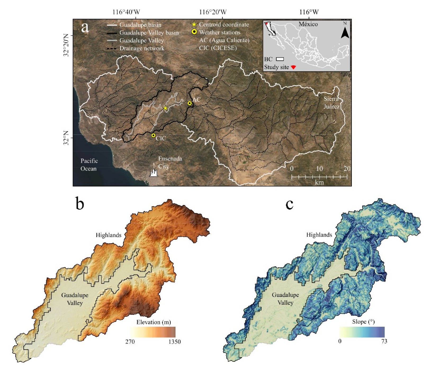
2.1. Study Area

The study area comprises the Guadalupe Valley Basin (GVB) (centroid coordinates; 32°06′01″ N, 116°33′13″ W), located 37 km north of the city of Ensenada in Baja California, Mexico (Figure 1a). Hydrographically, it includes the Guadalupe Valley and its aquifer (Guadalupe aquifer). The GVB comprises the central portion of a larger basin (Guadalupe Basin) with runoff flowing east-west (from the Sierra de Juárez to the Pacific Ocean). The geomorphology of the GVB (315 km²) is divided into the following two main areas: a zone with steep topography (highlands, 220 km²), mainly covered by natural vegetation (Chaparral), and a flat zone, dominated by an agricultural inter-mountain alluvial valley (95 km²), which constitutes the principal wine producing region in Mexico (Figure 1b,c).

The climate type is semi–arid Mediterranean [34], with rainfall during the cool–winters (December–March), dry warm–summers (June–September), and the hydrological year ranges from October to September. Annual precipitation varies from ca. 60 mm to 600 mm, and the average is ca. 264 mm y⁻¹. Approximately 77% of total rainfall falls in winter and around 2% in summer; the remaining 21% occurs in the other two intervening seasons. The average temperature varies from 13 °C in December to 25 °C in August and an annual 18.3 °C [12]. This region is included in the California Floristic Province, a hot spot of biological diversity. The main vegetation types in the GVB highlands are evergreen sclerophyllous chaparral and Diegan coastal sage scrub vegetation species [35,36]. The natural ecosystem presents low anthropogenic disturbance. The slope gradient (Slo) in the GVB was calculated using a 5–m digital elevation model (DEM) from the Mexican National Institute of Statistics and Geography (INEGI, [37]). The slope surface was reclassified considering a Slo ≤ 8° and Slo > 8° to fragment the agricultural valley and natural zones, and further visual inspection with Google Earth imagery and field observations. For the purpose of this study, GVB will refer only to hillslopes (highlands) above 8°. Elevation and slope gradient in the valley range from 270 to 460 m (average, 331 m) and 0–8° (average, 2°), excluding small hilly areas immersed on the valley surface with steeper slopes (Figure 1b,c). Elevation and slope gradients in the GVB range from 274 to 1350 m (average, 584 m) and 0–73° (average, 18°), including areas with slopes of less than 8° that occupy small valleys located in the highlands (Figure 1b,c). The dominant slope gradient in GVB ranges from 14 to 23°.

2.2. Meteorological–Based Drought Indices

Drought indices based on weather–station datasets have been used as agents for meteorological drought evaluation [2]. This research uses two of the most widely used drought indices for monitoring meteorological drought, the RDI and SPI. The RDI is based on the relationship between precipitation and potential evapotranspiration fluxes (Figure 2), thus providing a long–term trend for temperature and precipitation [8]. The SPI is calculated by fitting historical precipitation into a Gamma probability distribution function and re–transforming it to a normal distribution [7]. The data are fitted to a mean of zero in both indices and a standard deviation of one; this allows for identifying historical wet, dry, and neutral periods (positive, negative, and zero values, respectively) (

Table 1. Drought severity classification according to the Standardized Precipitation Index (SPI) modified from [7], applied to the classification of drought in the Guadalupe Valley Basin, Baja California, Mexico.

Drought Classification	SPI
Normal (NOR)	>−0.5
Abnormally dry (AD)	−0.5 to −0.8
Moderate drought (MD)	−0.8 to −1.3
Severe drought (SD)	−1.3 to −1.6
Extreme drought (ED)	−1.6 to −2
Exceptional drought (ExD)	<−2

).

RDI and SPI were calculated with monthly precipitation and potential evapotranspiration data (from mean temperature) obtained from the Agua Caliente (AC) weather station of the Mexican National Water Commission (CONAGUA) during the 1979–2016 period and the Guadalupe Valley (CIC) weather station of the Ensenada Center for Scientific Research and Higher Education (CICESE) for 2017–2018 period (location, Figure 1; data, Figure 2).

Potential evapotranspiration was calculated using monthly mean temperature with Thornthwaite’s methodology [38]. We tested the meteorological sensitivity and surface reflectance–derived spectral indices to drought conditions in the region on an annual (AN) and seasonal basis. Seasons were divided into wet (WS), dry (DS), and the following two intervening hydrological seasons (IS): IS1, October–November, WS, December–March, IS2, April–May, and DS, June–September [39]. In subsequent analyses, the precipitation, RDI, and SPI time–series from October 1992 to September 2018 were used congruently with Landsat time–series data (26 hydrological years, 1992/93–2017/18) per each of these seasons.

2.3. Imagery Processing

We compiled a terrain precision correction (L1TP) 30–m Landsat monthly dataset from October 1992 to September 2018, covering 26 hydrological years. Data were acquired from the U.S. Geological Survey (USGS) EarthExplorer website [40] (Landsat 5 TM, 1992–2011; Landsat 7 ETM+ and Landsat 8 OLI/TIRS from 2012–2018). In total, we processed 307 Landsat tiles Path 39/Row 38 and Path 40/Row 38 (<10% cloud cover) that encompassed the study area in QGIS 3.14.16 with GRASS 7.8.3 [41,42]. Moreover, a 5–m spatial resolution DEM from INEGI was used to delineate the basins, the hydrographic network, and hillslope zones within GVB (Figure 1).

Landsat datasets were missing data for six months (December 1994; February 1995; April 1999; November 2013; January 2014; December 2016) due to cloud cover and no data from the EarthExplorer platform. The original data (spectral bands) were corrected for atmospheric effects, and the original image format of Digital Numbers was converted to radiance and then into surface reflectance with the semi–automatic classification plug–in in QGIS 3.14.16 [43]. Moreover, inter–calibration of spectral bands between TM, ETM+, and OLI sensors was performed [44]. Then, we calculate the NDVI as the ratio between reflectance in the near–infrared (NIR) minus the reflectance of visible red (R) band of the electromagnetic spectrum and the sum of the NIR and R bands (NDVI = (NIR-R/NIR + R)) [23] and land surface emissivity by the logarithmic relationship between temperature emissivity and NDVI as described in [45]. The LST [46,47] was computed with the spectral radiance conversion to at–sensor brightness temperature, land surface emissivity, and NDVI. The details of the image preprocessing are described in

Table 2. Spectral bands preprocessing procedure. Radiometric and atmospheric corrections, brightness conversion to temperature, and the Normalized Difference Vegetation Index calculation steps for 307 tiles of Landsat. Datasets covered 26 hydrological years in the Guadalupe Valley Basin, Baja California, Mexico.

Image Conversion to Reflectance	Equation		Equation Notation
Spectral Radiance at the Sensor’s Aperture (Lλ) [43]	$\mathrm{L}\mathsf{\lambda }=\mathrm{ML}\ast \mathrm{DN}+\mathrm{AL}$	(1)	ML = Multiplicative rescaling factor AL = Additive rescaling factor DN = Digital number d = Earth-Sun distance ESUNλ = Mean solar exo-atmospheric irradiance θs = Solar zenith angle Lp = Path radiance DNmin = Minimum DN value K1, K2 = Band specific thermal constants λ = Mean wavelength of emitted radiance c2 = h ∗ c/s (1.4388 ∗ 10−2 m K) h = Plank’s constant (6.626 ∗ 10−34 J s) s = Boltzmann constant (1.38 ∗ 10−23 J K) c = Velocity of light (2.998 ∗ 108 m s−1)
Top of Atmosphere (TOA) Reflectance (ρp) [43]	$\mathsf{\rho }\mathrm{p}=\frac{\left(\mathsf{\pi }\ast \mathrm{L}\mathsf{\lambda }\ast {\mathrm{d}}^2\right)}{\mathrm{ESUN}\mathsf{\lambda }\ast \cos \mathsf{\theta }\mathrm{s}}$	(2)
Land Surface Reflectance (ρ) [43]	$\mathsf{\rho }=\frac{\left(\mathsf{\pi }\ast \left(\mathrm{L}\mathsf{\lambda }-{\mathrm{L}}_{\mathrm{p}}\right){\ast \mathrm{d}}^2\right)}{\mathrm{ESUN}\mathsf{\lambda }\ast \cos \mathsf{\theta }\mathrm{s}}$	(3)
Atmospheric correction	Equation
Dark Object Subtraction Method (DOS1) [43,48]	${\mathrm{L}}_{\mathrm{p}}=\frac{{\mathrm{ML}\ast \mathrm{DN}}_{\min }+\mathrm{AL}-0.01\ast \mathrm{ESUN}\mathsf{\lambda }\ast \cos \mathsf{\theta }\mathrm{s}}{{\mathsf{\pi }\ast \mathrm{d}}^2}$	(4)
Brightness conversion to Temperature	Equation
Satellite Brightness Temperature (TB) [43]	$\mathrm{TB}=\frac{{\mathrm{K}}_2}{\ln \left[\left({\mathrm{K}}_1/\mathrm{L}\mathsf{\lambda }\right)+1\right]}$	(5)
Land Surface Temperature (LST) [46]	$\mathrm{LST}=\frac{\mathrm{TB}}{\left[1+\left(\mathrm{TB}/{\mathrm{c}}_2\right)\ast \ln \left(\mathrm{e}\right)\right]}$	(6)
Land Surface Emissivity (e) [45]	$\mathrm{e}=1.009+0.047\ast \ln \left(\mathrm{NDVI}\right)$	(7)
Surface reflectance vegetation index	Equation
Normalized Difference Vegetation Index (NDVI) [23]	$\mathrm{NDVI}=\frac{\mathrm{NIR}-\mathrm{R}}{\mathrm{NIR}+\mathrm{R}}$	(8)

. To avoid human disturbances (e.g., irrigation), we eliminated the agricultural land (flat slopes within GVB); then, each image was clipped to the GVB boundaries to obtain the hillslope surface of the GVB. Monthly Landsat bands were stacked, and surface reflectance–derived spectral indices were calculated per dataset (NDVI, VCI, TCI, VHI, MSAVI, NDWI).

2.4. Surface Reflectance–Derived Spectral Indices

Using corrected Landsat data, the biophysical responses of the vegetation to annual and seasonal climatic conditions, precipitation, and potential evapotranspiration fluxes included in the RDI and SPI calculation were represented by the values of the NDVI [23], the LST [46], the VCI, the TCI, the VHI [27], the MSAVI [29] and the NDWI [31]. The VCI and TCI were estimated from NDVI and LST values following the procedure illustrated in Table 2.

$$\mathrm{VCI}=\frac{\mathrm{NDVI}-{\mathrm{NDVI}}_{\left(\min \right)}}{{\mathrm{NDVI}}_{\left(\max \right)}-{\mathrm{NDVI}}_{\left(\min \right)}}$$

(9)

The VCI equation relates the NDVI values in a determined period using the long–term minimum NDVI value (NDVI_(min)), normalized by the range of NDVI values calculated in the same period.

$$\mathrm{TCI}=\frac{{\mathrm{LST}}_{\left(\max \right)}-\mathrm{LST}}{{\mathrm{LST}}_{\left(\max \right)}-{\mathrm{LST}}_{\left(\min \right)}}$$

(10)

The TCI equation was formulated in reversed quotient to the VCI where LST_(max) and LST_(min) are the long–term maximum and minimum LST values in a defined period, based on the assumption that higher temperatures would fare worst for the vegetation development, and vice versa [24]. A combination of VCI and TCI to form VHI has proven to be a valuable tool for meteorological and agricultural drought detection in climatic regions where water availability is the main restriction for the development of natural vegetation (arid, semi–arid, and sub–humid zones) [13,27,49,50,51]. We assigned an α value of 0.5, assuming an even contribution from both indices (VCI, TCI) in the VHI [52] to drought classification.

$$\mathrm{VHI}=\mathsf{\alpha }\mathrm{VCI}+\left(1-\mathsf{\alpha }\right)\mathrm{TCI}$$

(11)

The MSAVI was proposed to correct the soil factor (L) in the Soil Adjusted Vegetation Index (SAVI, [53]), minimizing soil background reflectance in vegetation spectral signature [29]. MSAVI was developed aiming to produce a more reliable indicator of vegetation spectral signature than NDVI on deciduous vegetation surfaces [29,54]. Therefore, it could be a better indicator of vegetation greenness and response to meteorological drought in sparse vegetation sites than NDVI, VCI, and VHI. In equation 4, NIR and R are the near–infrared and red reflectance bands, respectively.

$$\mathrm{MSAVI}=\frac{2\mathrm{NIR}+1-\sqrt{{\left(2\mathrm{NIR}+1\right)}^2-8\left(\mathrm{NIR}-\mathrm{R}\right)}}{2}$$

(12)

We also included the NDWI because it is considered a reflectance–based water–sensitive vegetation index [31]. The NDWI was calculated as the ratio between reflectance in the near–infrared (NIR) minus the reflectance of the short–wave infrared (SWIR) band of the electromagnetic spectrum and the sum of the NIR and SWIR bands.

$$\mathrm{NDWI}=\frac{\mathrm{NIR}-\mathrm{SWIR}}{\mathrm{NIR}+\mathrm{SWIR}}$$

(13)

2.5. Statistical Analyses

Mean monthly and seasonal (IS1, WS, IS2, DS, AN) surface reflectance–derived indices values were calculated and extracted with the Zonal Statistics function. The strength and direction of linear relationships between surface reflectance–derived indices and meteorological drought indices were evaluated by means of correlation coefficients (R), using Pearson correlations, either in a seasonal or annual time frame for the entire period (October 1992 to September 2018), only for hillslopes within the GVB. A standardized deviation from the long–term mean was calculated to find anomalies in the surface reflectance–derived indices by applying the Standardized Anomaly Index (SAI) [55]. Lastly, we compare the seasonal response of vegetation with the meteorological drought indices (RDI, SPI) as follows:

$${\mathrm{SAI}}_{\mathrm{i}}=\frac{{\mathrm{x}}_{\mathrm{i}}-\overline{\mathrm{x}}}{\mathsf{\sigma }}$$

(14)

where x_i, $\overline{\mathrm{x}}$, and σ are the seasonal mean of reflectance–based indices, the long–term mean, and the standard deviation, respectively. Then, simple linear regression models were developed with the surface reflectance–derived spectral indices best correlated with RDI and SPI in hydrological seasons to apply a per–pixel correction and establish the drought–affected area in the GVB highlands during 1992/93–2017/18 hydrological years.

3. Results

3.1. Linking Climatic and Biophysical Parameters

In the Guadalupe Valley Basin (GVB), during the study period (October 1992–September 2018), the occurrence of meteorological droughts comprised time intervals with high temperatures and low precipitation. Drought periods were successfully visualized by the monthly and seasonal time–series of the NDVI, and LST hillslopes values, as well as the daily and seasonal precipitation datasets from Agua Caliente and CICESE weather stations (Figure 3).

The NDVI values from each season provided information on the GVB’s historical and recent greenness variability. Figure 3a shows the time series of NDVI calculated with Landsat 5, 7, and 8 datasets. From 2013 onwards, the NDVI values were calculated with Landsat 8 (dark green line) and Landsat 7 (light green line). Oddly, the Landsat 8 NDVI values from 2013 onwards increased after the inter–calibration process, which does not coincide with the daily (Figure 3c) and seasonal (Figure 3f) precipitation records. Therefore, all further analyses and results are presented from the Landsat 5 and 7 datasets. We corrected the Landsat 7 striped band errors with the GRASS 7.8.3 r.fillnulls function included in QGIS 3.14.16 [41,42]. The NDVI values showed a seasonal progression with peak values during IS2 (April–May), WS (December–March) and a minimum through IS1 (October–November), DS (June–September) (Figure 3a,d), which are inverse to the LST values. Overall, NDVI peak values (NDVI ≥ 0.4) occurred at the end of WS and during IS2 (e.g., 1992/93, April; 1995/96, March; 1997/98, April; 2000/01, April; 2012/13, March; 2016/17, March), preceded by the maximum accumulated rainfall during WS of 146–504 mm (Figure 3f) and the lowest LST values (on average 13–23 °C) (Figure 3b), due to the delay of biomass production. Lower NDVI values (NDVI ≤ 0.2) occurred regularly between June and July and remained nearly constant from months (e.g., July 97 to September 97) to years (e.g., April 02–February 03, July 05–January 08, June 13–January 15) (Figure 3a). In those periods, precipitation in WS did not exceed 125 mm, and maximum LST values identified mainly in DS, and IS2 ranged from 31 to 36 °C (Figure 3e). Overall, lower NDVI values (Figure 3a,d) strongly corresponded with the driest hydrological wet seasons and years. For instance, WS precipitation in 2001/02 (54 mm), 2005/06 (74 mm), 2006/07 (65 mm), 2013/14 (48 mm), 2017/18 (49 mm). In the studied climatic period (1992–2018), the 2017/18 hydrological year stands as the driest year in our record (annual precipitation = 58 mm) (Figure 3c,f).

3.2. Seasonal and Annual Correlations

There were strong correlations between seasonal NDVI, LST, and precipitation (

Table 3. Seasonal Pearson’s correlation coefficients between the Land Surface Temperature (LST), the Normalized Difference Vegetation Index (NDVI), and Precipitation (P) in the Guadalupe Valley Basin, Baja California, Mexico.

P						P						LST
LST	IS1	WS	IS2	DS	AN	NDVI	IS1	WS	IS2	DS	AN	NDVI	IS1	WS	IS2	DS	AN
IS1	−0.18	−0.20	−0.07	−0.33	−0.25	IS1	0.07	−0.03	0.00	0.47	0.02	IS1	−0.25	−0.36	−0.08	−0.18	−0.15
WS	−0.28	−0.82	−0.17	−0.28	−0.82	WS	0.41	0.69	0.02	0.33	0.73	WS	−0.51	−0.24	−0.54	−0.32	−0.33
IS2	−0.06	−0.59	−0.34	−0.23	−0.59	IS2	0.20	0.78	0.28	0.31	0.78	IS2	−0.72	−0.20	−0.64	−0.54	−0.62
DS	−0.01	−0.59	−0.47	−0.37	−0.60	DS	0.11	0.76	0.25	0.32	0.74	DS	−0.68	−0.26	−0.59	−0.49	−0.63
AN	−0.21	−0.74	−0.36	−0.42	−0.77	AN	0.28	0.79	0.17	0.40	0.81	AN	−0.70	−0.28	−0.63	−0.49	−0.56
				Strong			Moderate				Weak			Negligible

). For instance, LST and precipitation negatively co–vary for WS and AN (R = −0.74–−0.82), resulting in lower LST values during rainy periods. Moreover, strong positive correlations (from R = 0.73 to 0.81) between NDVI and precipitation were found in AN, IS2, WS, and DS. Water availability enhanced vegetation greening responses during (WS), development (IS2), and water shortage (DS), which diminished greenness throughout the hydrological seasons (Table 3). Seasonal and annual variation in vegetation greenness (NDVI, Figure 3a,d) and its correlation with precipitation and LST showed a clear positive linear response with precipitation (WS R = 0.69; AN R = 0.81) and moderate–weak negative associations with LST (WS R = −0.24; AN R = −0.56). Both factors (precipitation and LST) affected the NDVI (positively/negatively), but the correlations pointed to precipitation as the primary seasonal control on NDVI more than LST.

The Pearson’s correlation coefficient analysis of five surface reflectance–derived spectral indices (NDVI, LST, VHI, MSAVI, NDWI) with the meteorological drought indices (RDI, SPI) across the hydrological seasons showed a consistently higher correlation for MSAVI than for VHI, NDWI, NDVI, and finally LST (

Table 4. Seasonal Pearson correlation coefficients (Annual, AN; Intervening Season 1, IS1; Wet Season, WS; Intervening Season 2, IS2; Dry Season, DS) for vegetation/water indices (Normalized Difference Vegetation Index, NDVI; Land Surface Temperature, LST; Vegetation Health Index, VHI; Normalized Difference Water Index, NDWI; Modified Soil Adjusted Vegetation Index, MSAVI) and meteorological drought indices (Reconnaissance Drought Index, RDI; Standardized Precipitation Index, SPI) in the Guadalupe Valley Basin, Baja California, Mexico. p-Value < 0.01 for all cases.

	NDVI					LST					VHI
Seasons	AN	IS1	WS	IS2	DS	AN	IS1	WS	IS2	DS	AN	IS1	WS	IS2	DS
RDI AN	0.80	0.00	0.73	0.79	0.73	−0.78	−0.26	−0.83	−0.59	−0.60	0.86	0.19	0.86	0.81	0.75
RDI IS1	0.33	0.17	0.41	0.24	0.18	−0.26	−0.23	−0.33	−0.11	−0.08	0.33	0.25	0.43	0.22	0.17
RDI WS	0.80	0.01	0.73	0.77	0.74	−0.74	−0.26	−0.79	−0.55	−0.54	0.84	0.19	0.85	0.78	0.74
RDI IS2	0.10	0.00	−0.03	0.22	0.16	−0.38	−0.14	−0.16	−0.40	−0.45	0.21	0.09	0.04	0.32	0.27
RDI DS	0.40	0.31	0.33	0.36	0.35	−0.45	−0.37	−0.35	−0.19	−0.40	0.45	0.42	0.37	0.33	0.39
SPI AN	0.78	−0.03	0.72	0.77	0.71	−0.77	−0.26	−0.82	−0.58	−0.60	0.84	0.17	0.84	0.79	0.74
SPI IS1	0.31	0.12	0.40	0.23	0.17	−0.23	−0.16	−0.32	−0.09	−0.09	0.30	0.17	0.42	0.20	0.16
SPI WS	0.78	−0.09	0.69	0.77	0.74	−0.76	−0.20	−0.82	−0.59	−0.61	0.83	0.10	0.83	0.80	0.76
SPI IS2	0.09	−0.04	−0.05	0.22	0.16	−0.36	−0.11	−0.16	−0.37	−0.43	0.20	0.06	0.02	0.31	0.26
SPI DS	0.36	0.34	0.30	0.29	0.30	−0.41	−0.41	−0.30	−0.16	−0.35	0.40	0.46	0.33	0.27	0.34
	NDWI					MSAVI					Correlation level
Seasons	AN	IS1	WS	IS2	DS	AN	IS1	WS	IS2	DS
RDI AN	0.82	0.15	0.75	0.88	0.68	0.88	0.03	0.67	0.90	0.84			Very Strong
RDI IS1	0.49	0.03	0.54	0.41	0.37	0.43	0.10	0.50	0.32	0.29			Strong
RDI WS	0.74	0.17	0.67	0.83	0.60	0.87	0.05	0.66	0.87	0.83			Moderate
RDI IS2	0.30	−0.07	0.19	0.30	0.44	0.15	−0.12	−0.01	0.24	0.26			Weak
RDI DS	0.03	−0.40	−0.02	0.23	0.09	0.24	−0.04	0.11	0.30	0.27			Negligible
SPI AN	0.81	0.12	0.73	0.89	0.69	0.85	−0.03	0.65	0.88	0.82
SPI IS1	0.50	−0.01	0.54	0.42	0.39	0.42	0.04	0.49	0.32	0.28
SPI WS	0.77	0.13	0.68	0.88	0.65	0.85	−0.04	0.61	0.89	0.83
SPI IS2	0.27	−0.08	0.17	0.28	0.41	0.14	−0.17	−0.02	0.24	0.25
SPI DS	−0.02	−0.43	−0.07	0.19	0.07	0.19	−0.04	0.09	0.23	0.21

). In seasonal terms, surface reflectance–derived spectral indices presented the weakest correlations in IS1 (October–November) and the highest association in AN (annual) and IS2 (April–May). Meteorological drought indices presented the lowest association in both intervening seasons and in DS (June–September) and the most robust correlations during AN and WS (December–March). Overall, surface reflectance–derived vegetation indices MSAVI, NDWI, and VHI consistently showed stronger associations (R = 0.73–0.90) with meteorological drought indices (RDI AN, WS; SPI AN, WS) across almost all hydrological seasons (WS, IS2, DS, AN). Due to RDI and SPI’s close relationship with precipitation, the strongest correlations between LST–RDI and LST–SPI occurred during WS and AN (R = −0.74–−0.83). The robust associations between NDWI–RDI and NDWI–SPI were found mainly during seasons with high water availability (WS, IS2) and in the annual context (R = 0.73–0.89) (Table 4).

3.3. Meteorological–Based and Surface Reflectance–Derived Drought Indices

Per–pixel surface reflectance–derived spectral indices were standardized with the long–term average and standard deviation in VHI AN, NDWI IS2, and MSAVI IS2 (Figure 4).

The meteorological drought indices (RDI, SPI) did not show representative differences in their values. Positive/negative values indicate wet/dry years, respectively. Consecutive wet years are infrequent and only occurred in 2009/10–2011/12, while periods with several dry years were more frequent (1995–1997, 1998–2000, 2001–2004, 2005–2009, 2012–2016). The results indicate that the duration of dry periods was increased for the studied years. The driest hydrological years from 1992 to 2018 were 2001/02, 2006/07, 2013/14, and 2017/18 (Figure 4). The surface reflectance–derived spectral drought indices that showed higher correlations with RDI and SPI (VHI, NDWI, MSAVI) were included in a multiple regression analysis, indicating that they are robust to predicting RDI and SPI in selected hydrological seasons (multiple R² = 0.86–0.90, adjusted R² = 0.73–0.81, with p-Values far lower than 0.01) (

Table 5. Linear regression models for three selected surface reflectance-derived drought indices (VHI, NDWI, MSAVI) and seasons (intervening season 2, IS2; annual, AN) and the annual meteorological drought indices (Reconnaissance Drought Index, RDI; Standardized Precipitation Index, SPI) to assess drought classification, affected area, and duration at the Guadalupe Valley Basin, Baja California, Mexico.

Variable	Multiple R	Adjusted R	Intercept (I)	Coefficient (C)	p-Values
VHI AN–RDI AN	0.86	0.73	−5.2862	12.7159	1.82 × 10−8 (I); 2.34 × 10−8 (C)
NDWI IS2–SPI AN	0.89	0.79	0.9202	13.8414	1.52 × 10−6 (I); 1.07 × 10−9 (C)
MSAVI IS2–RDI AN	0.90	0.81	−3.9754	26.9899	2.27 × 10−10 (I); 2.74 × 10−10 (C)

). The IS2 standardized values of NDWI and MSAVI were selected to obtain the RDI AN and SPI AN predictor values to perform pixel–correction and establish the spatial extension of meteorological drought on the GVB during the study period (NDWI in Figure 5; MSAVI in Figure 6).

3.4. Surface Reflectance–Derived Drought Assessment

The drought severity classification and drought–affected areas were calculated based on standardized NDWI IS2 and MSAVI IS2 predicted values from 1992/93 to 2018/19 hydrological years. Both drought classification maps (Figure 5 and Figure 6) agree on the detection of drought trends. The spatial patterns of drought were classified according to SPI class values in Table 1, from exceptional drought to normal conditions (from light to dark colors). Seasonal and annual differences (dry/wet years) can be monitored with surface reflectance–derived vegetation/water indices (Table 3). In the MSAVI IS2 historical record (Figure 6), the drought–affected area in the GVB (Figure 7) showed only seven years of normal hydrological conditions, according to Table 1. Under normal conditions, a relatively stable period occurred between 2007/08 and 2011/12 (five years). Dry conditions affected at least 50% of the GVB surface for 11 years in two–year cycles during 1995/96–2006/07, interrupted by years with annual precipitation ≥ 245 mm (historical mean, Figure 3f). Then, a sequence of dry years occurred from 2012/13 to 2015/16 and 2017/18 (Figure 7). The driest ten–year sequence affected a high percentage of the GVB area. The overall GVB area affected by moderate to exceptional drought during this extreme anomaly ranged from 99% in 2017/18, 96% in 2006/07, 87% in 2013/14, 73% in 2005/06, and 58% in 2014/15 (Figure 7). A fire scar (ca. 11 km²) was detected during the period of 2006/07–2007/08 in the southern limit of the GVB, and by 2008/09, the vegetation apparently recovered (Figure 5 and Figure 6).

4. Discussion

Traditional drought monitoring methods based on ground–weather observations depend entirely on weather station data. Incomplete data series and the absence of a continuous record of the spatial extent of droughts are common issues in Mexico [56,57,58]. Given that the vegetation development throughout the hydrological year is sensitive to climatic variation (temperature and precipitation) [59,60], Landsat’s long–term observations allowed us to derive the surface reflectance–derived spectral indices and to observe changes in vegetation reflectance induced by meteorological droughts. The strong correlations between the surface reflectance–derived spectral indices MSAVI, NDWI, and VHI with both meteorological drought indices (RDI, SPI) (Table 4) allowed us to quantify the drought–affected hillslope area across the Guadalupe Valley Basin (GVB) over a time span of 26 years. Therefore, this procedure is suitable to be used to determine the spatial and temporal trends of meteorological drought in areas lacking adequate coverage of weather stations.

4.1. Seasonal and Annual Responses of NDVI to Precipitation and LST

Temperature and precipitation are the main climatic factors that produce changes in soil water content and thus modulate vegetation growth and health [59,61]. The NDVI has been frequently used to study vegetation dynamics in arid and semi–arid areas, the degree of aridity, and desertification and to assess meteorological drought due to its relationship with climatic factors (e.g., LST, precipitation) [18,20,62,63,64]. Significant associations between NDVI–LST and NDVI–precipitation in all hydrological seasons reflect the tight control of vegetation reflectance on the upper layer of soil water content [65]; however, there is wide variability, particularly when the water content is lower, which results in a lowering of the strength of the correlation between seasonal NDVI–LST. [39] showed that surface soil water content (ca. 0.4 m) in the mountainous regions of this same study area is enriched during the wet season (WS) and almost totally depleted towards the end of the dry season (DS). We found low negative seasonal NDVI–LST correlations, implying a weak control of temperature on vegetation greenness. Therefore, it is the lack of soil water availability at the beginning of the hydrological year (IS1) and the gradual replenishment of soil water content in WS that is the main correlate of greenness. With the increase in soil water content by precipitation in WS, the degree of correlation between NDVI–LST tends to increase because of the peak of vegetation development and greenness (IS2) and, later, the gradual reduction of the soil water content by the end of the hydrological year (DS) (Table 3). In mid–latitude semi–arid and drylands, the relationships between NDVI and LST typically show negative correlations [66,67], and vegetation greenness (NDVI), cover, and density are usually linked with LST changes [49,50,51,68,69]. Although correlations showed that LST still exerts a relevant control on the availability of soil water for vegetation development in the GVB highlands, the distribution of precipitation over the hydrological seasons (WS, IS2, DS, AN) exerts a much greater positive control related to the evolution of NDVI (Table 3). Moreover, variations in precipitation during WS and across the years (Figure 3f) were reflected in the seasonal NDVI values (Figure 3d) better than LST (Figure 3e).

4.2. Relationships between Surface Reflectance–Derived Spectral Indices and Meteorological Drought Indices

The NDVI–AN and NDVI–IS2 are strongly associated with meteorological indices RDI–WS, AN, and SPI–WS, AN (Table 4); however, climatic–related temporal changes in the drought assessment using only NDVI variations could lead to misinterpretations [27]. Therefore, we include the VHI, NDWI, and MSAVI in the meteorological drought assessment. VHI is a derivative of the inverse relationship between NDVI and LST. If positive correlations between NDVI and LST are found, the VHI indicates an energy–limited rather than a soil water–limited region [48,70], and the VHI is inadequate for meteorological drought monitoring [71]. In our dataset, we found negative correlations between NDVI and LST, and thus, the VHI adequately described the acclimation of the vegetation to precipitation and temperature over the study period. VHI preserved the seasonal pattern of NDVI values but increased the degree of association with meteorological drought indices (RDI and SPI) in all hydrological seasons, particularly during AN and IS2 (Table 4). Therefore, VHI results for the GVB support previous studies that identified a strong correlation between meteorological drought indices and hydrological variables (e.g., [13,70,71,72]).

Although not as popular as NDVI and VHI for meteorological drought monitoring, NDWI and MSAVI were the indices with the most robust correlations with meteorological drought indices, especially during WS and annually in the GVB (Table 4). NDWI has been found to be responsive to variations in plant leaf water content and soil moisture, being useful for monitoring drought status from agricultural [32] and natural vegetation at different spatial and temporal scales [57,72,73]. The MSAVI has been less used for meteorological drought detection than the other indices evaluated in this research [57]. However, MSAVI effectively responds to chlorophyll content changes within the intracellular spaces of leaves [29,74] and strongly colligated surface reflectance vegetation seasonal variation to meteorological indices (Table 4). Moreover, it prevented the vegetation spectral signature from being distorted by background soil surface reflectance, a common effect in arid and semi–arid regions [75] because of the low vegetation cover present in some areas (e.g., south–facing slopes, such as in the GVB highlands). Interestingly, the strongest associations between NDWI and MSAVI with RDI and SPI were found after WS, during IS2 due to the delay of growth in natural vegetation to reach the growing peak development and greenness after WS. Standardizing MSAVI, NDWI, and VHI with the meteorological indices (RDI, SPI) during the seasons with higher correlation (IS2, AN) (Figure 4), revealed that MSAVI and NDWI were more sensitive to meteorological drought monitoring in the study area. This advantage allowed us to model the spatial drought distribution and classify the drought severity (Table 1) in the GVB (Figure 5 and Figure 6).

4.3. Surface Reflectance–Derived Spectral Indices and Climatic Variations

The temporal and spatial variation in the surface reflectance–derived spectral indices suggest that the occurrence of dry years and periods in the GVB were due to reductions in precipitation during the wet season. In this region, intra–annual and inter–annual variations in precipitation have been associated with El Niño/Southern Oscillation (ENSO) and the Pacific Decadal Oscillation [76,77,78,79]. For instance, in the NW–Mexico and SW–U.S., ENSO (El Niño warm phase) coincided with the hydrological years 1992/93, 1994/95, 1997/98, 2004/05, 2009/10, and 2016/17, and the most severe dry effect of ENSO (La Niña cold phase) occurred in 2001/02, 2005/07, 2013/14, 2017/18 in the GVB (Figure 5 and Figure 6) (ENSO data, [80]). According to [12], regional climatic gradual changes have occurred in the last ca. twenty years due to the reduction of precipitation in the wet season and annual total precipitation patterns. This is coincident with the mega–drought of the beginning of the 21st century in California, a period of time in which recurring dry periods were common, and the effects were highly apparent at the GVB. For instance, in 2000–2002, abnormally dry years affected the SW–U.S. and NW–Mexico [15], and 2001/02 stood as the driest year in recorded history in southern California until 2007 [81]. A severe drought occurred from 2007 to 2009 in California [82], and an exceptional drought period befell between 2012 and 2014 [83]. Moreover, 2018 was the third warmest year in the Mexican historical record since 1953 [84] and the driest in the GVB region during the study period (Figure 3f). The drought impacts were observed on the GVB surface during those years (Figure 5 and Figure 6).

Although the results of this study revealed the extent of meteorological droughts in the GVB highlands, there are still limitations associated with the present study. Climatic factors are the main controls on the development and variation of the spectral signature of natural vegetation, which allows us to establish a relationship with meteorological drought. However, the relationship between meteorological drought and the spectral signature of plant communities is subject to uncertainty due to aspect (orientation) (e.g., evergreen vegetation, north–facing slopes; deciduous vegetation, south–facing slopes) and other possible sources of variation. Future research could provide more detail on surface reflectance–derived spectral indices applied specifically to vegetation/aspect types and soil moisture variation and describe the particular effect of meteorological drought modulated by aspect within this region.

5. Conclusions

This paper explored the long–term seasonal relationship between climatic (precipitation, LST) and biophysical (NDVI) parameters, and the long–term seasonal relationship between surface reflectance–derived spectral indices (NDVI, LST, VHI, NDWI, MSAVI) with meteorological drought indices (RDI, SPI) to assess and monitor drought in the Guadalupe Valley Basin highlands. Our main findings were as follows:

(a)

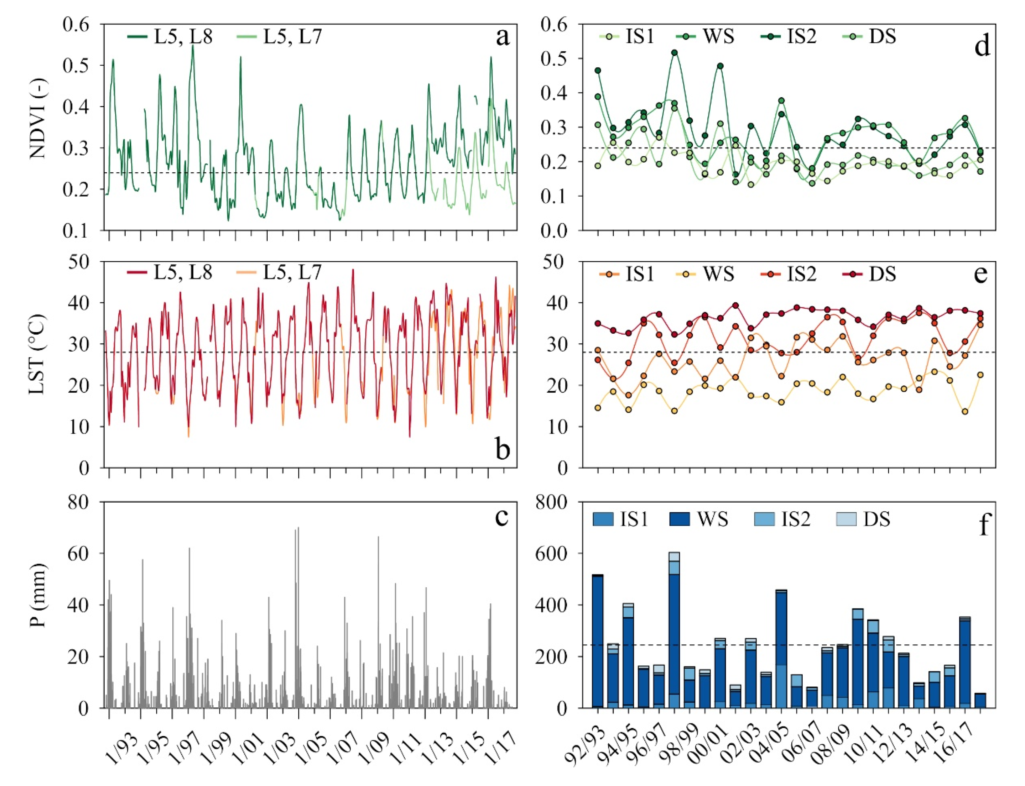
Both precipitation and LST factors affect the NDVI (positively/negatively), but stronger correlations revealed that precipitation is the primary seasonal control on NDVI across the hydrological seasons in the study area;

(b)

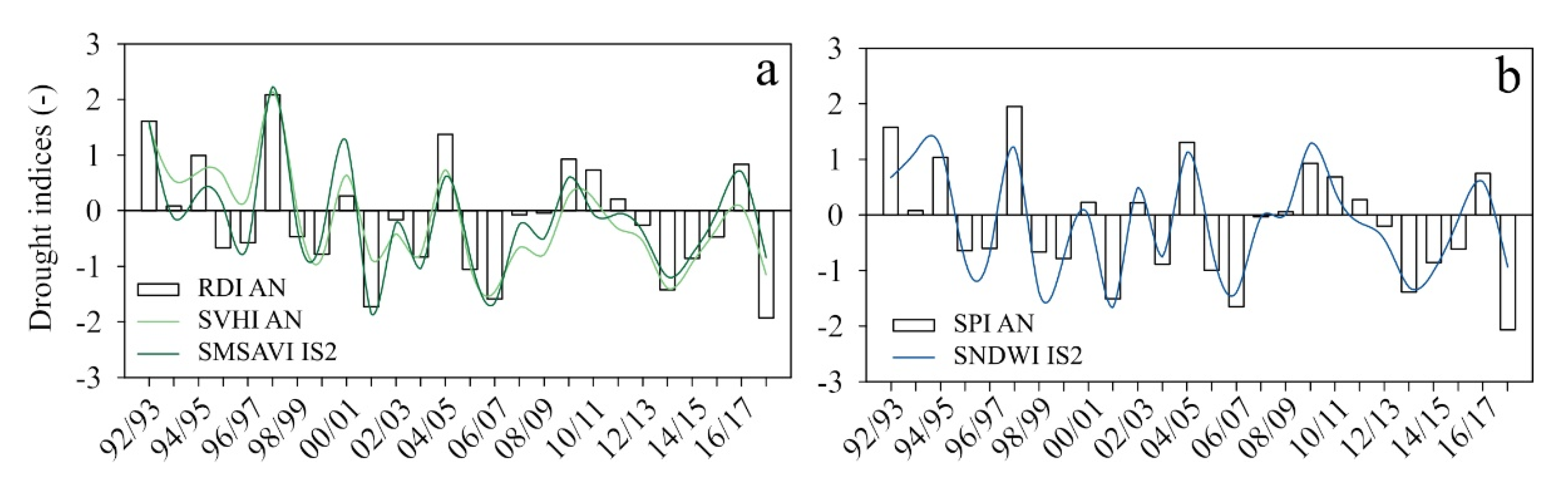
The VHI, NDWI, and MSAVI consistently showed stronger associations (R = 0.71–0.90) with meteorological drought indices (RDI AN, WS; SPI AN, WS) across almost all hydrological seasons (WS, IS2, DS, AN);

(c)

The strong correlations between VHI AN, NDWI IS2, and MSAVI IS2 with RDI AN and SPI AN suggest that this set of surface reflectance–derived spectral indices are the best predictors of meteorological drought in the GVB (Table 4);

(d)

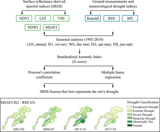
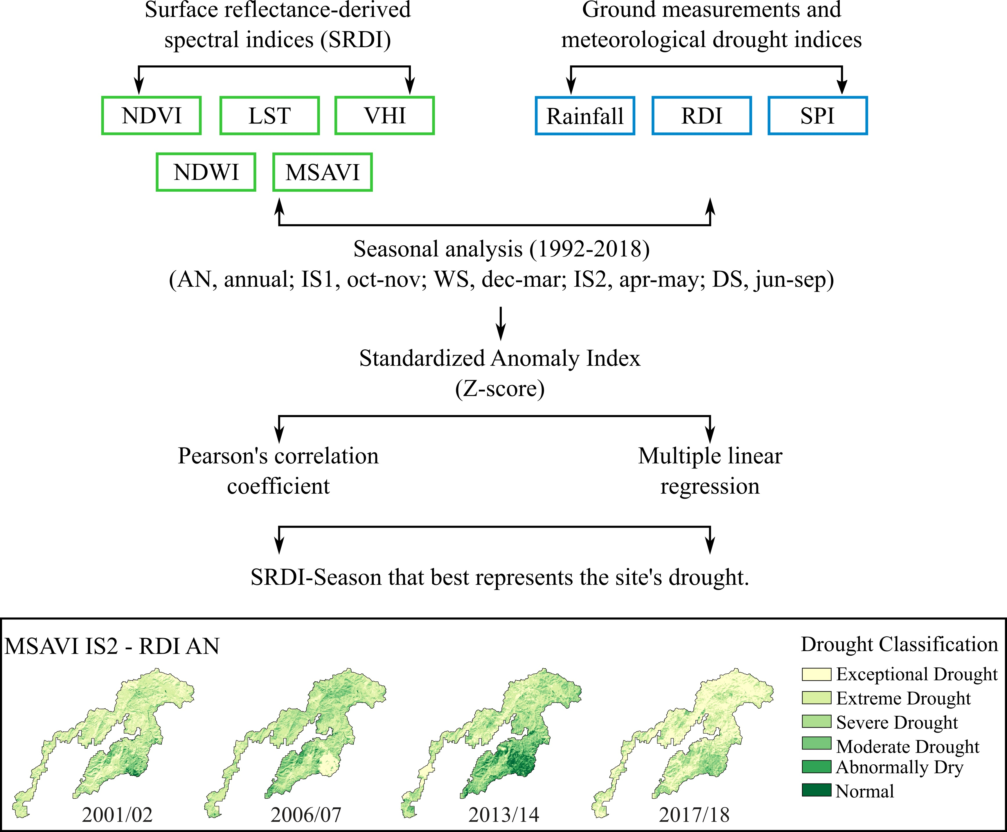
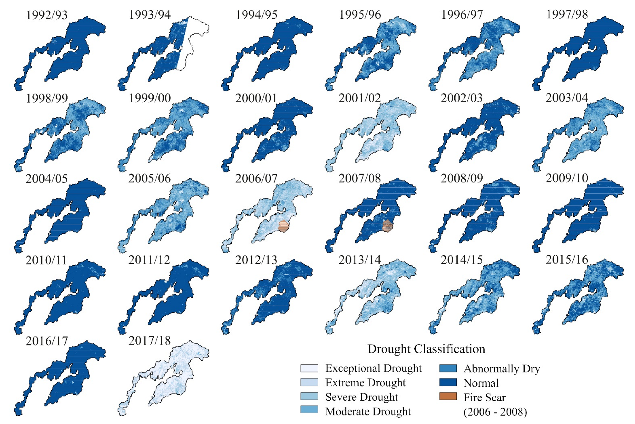
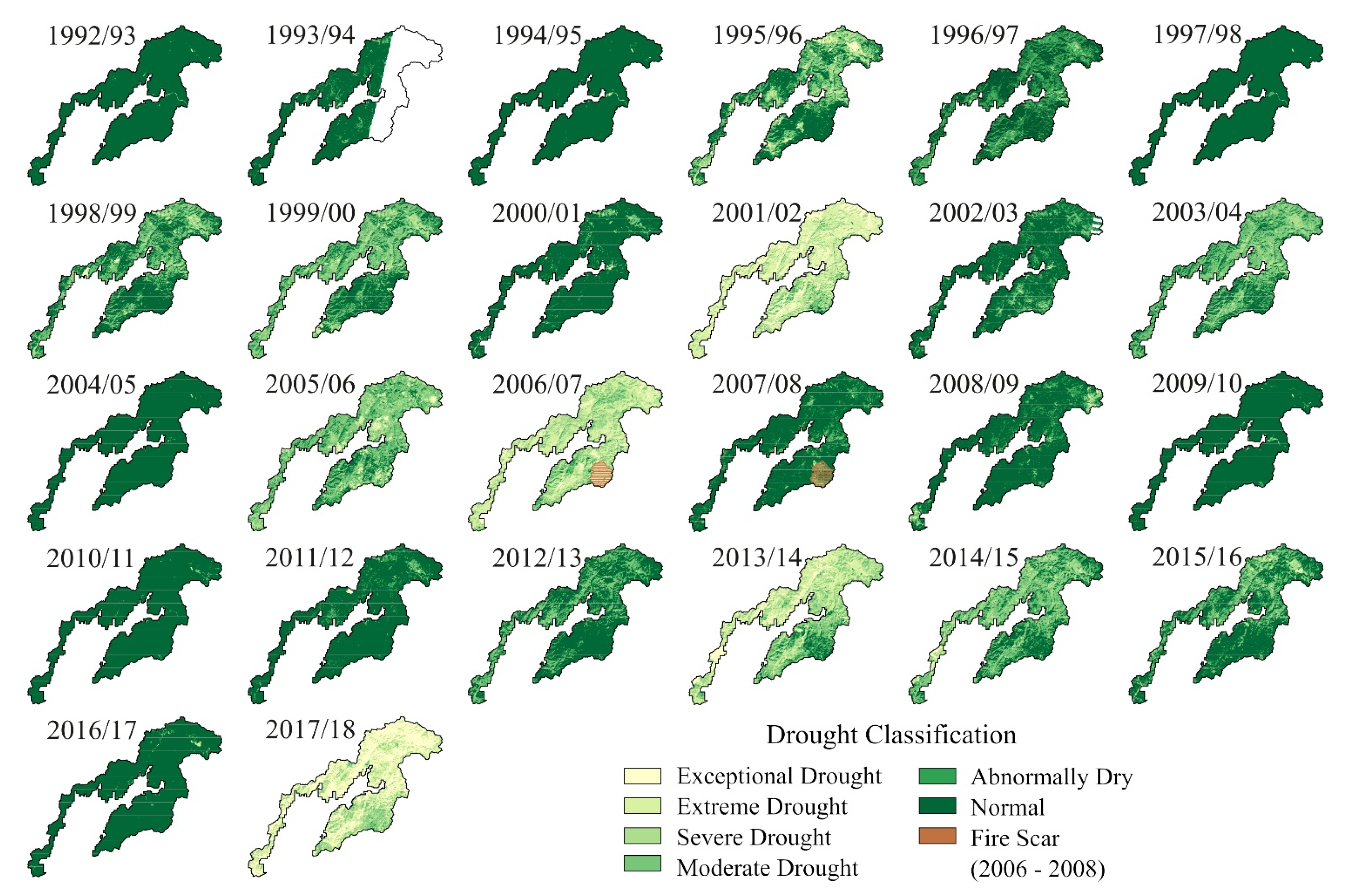
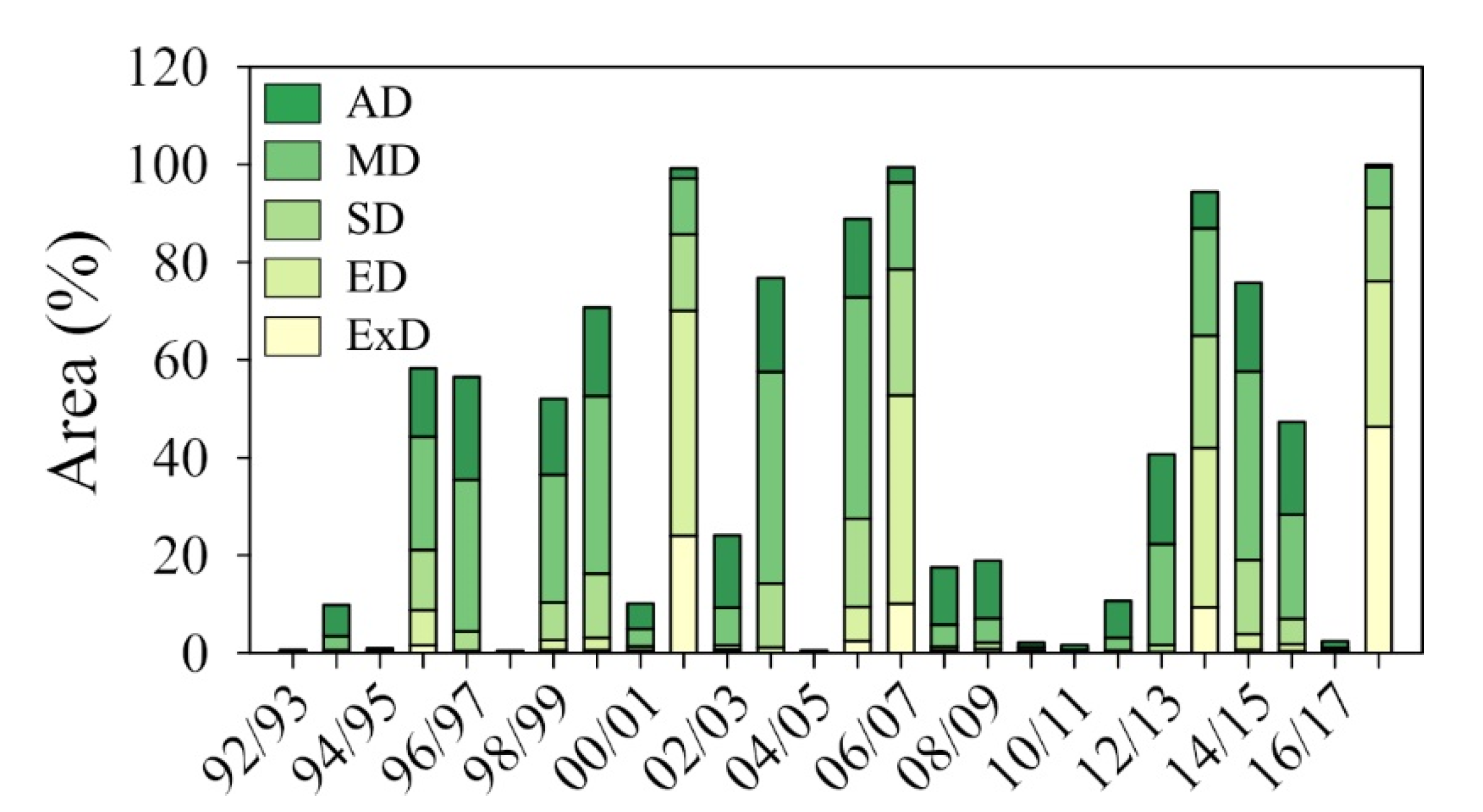
The maps generated from MSAVI and NDWI in the GVB (Figure 5 and Figure 6) adequately reproduce the dry/wet periods in the region. For instance, the worst dry years that affected the GVB area were 2017/18 (99%), 2001/02 (97%), 2006/07 (96%), and 2013/14 (87%), and coincided with extreme drought periods documented in the literature.

Given the limited availability of weather stations in this region, the spatial impact of drought would have been almost impossible to detect, so the integration of satellite–based observations and spectral indices derived from surface reflectance provides a valuable tool for establishing policies to mitigate and adapt to future climate anomalies. In particular, the spectral indices MSAVI, NDWI, and VHI were suitable indicators of meteorological drought using long–term data. These indices complement the weather station data in drought assessment, allowing more accurate modeling of the drought–affected area in the GVB and other areas subject to similar climatic conditions without adequate weather records.

References

1. Tsakiris, G.; Pangalou, D. Drought Characterisation in the Mediterranean. In Coping with Drought Risk in Agriculture and Water Supply Systems; Iglesias, A., Cancelliere, A., Wilhite, D.A., Garrote, L., Cubillo, F., Eds.; Springer: Dordrecht, The Netherlands, 2009; Volume 26, pp. 69–80. [Google Scholar]
2. Mishra, A.K.; Singh, V.P. A Review of Drought Concepts. J. Hydrol. 2010, 391, 202–216. [Google Scholar] [CrossRef]
3. Dai, A. Drought under Global Warming: A Review: Drought under Global Warming. WIREs Clim. Chang. 2011, 2, 45–65. [Google Scholar] [CrossRef] [Green Version]
4. Wilhite, D.A.; Svoboda, M.D.; Hayes, M.J. Understanding the Complex Impacts of Drought: A Key to Enhancing Drought Mitigation and Preparedness. Water Resour. Manag. 2007, 21, 763–774. [Google Scholar] [CrossRef] [Green Version]
5. Riebsame, W.E. Drought and Natural Resources Management in the United States: Impacts and Implications of the 1987–89 Drought; Routledge: New York, NY, USA, 2020. [Google Scholar]
6. Jain, S.K.; Keshri, R.; Goswami, A.; Sarkar, A. Application of Meteorological and Vegetation Indices for Evaluation of Drought Impact: A Case Study for Rajasthan, India. Nat. Hazards 2010, 54, 643–656. [Google Scholar] [CrossRef]
7. McKee, T.B.; Doesken, N.J.; Kleist, J. The Relationship of Drought Frequency and Duration to Time Scales. In Proceedings of the 8th Conference on Applied Climatology, Anaheim, CA, USA, 17–22 January 1993; Volume 17. [Google Scholar]
8. Tsakiris, G.; Vangelis, H. Establishing a Drought Index Incorporating Evapotranspiration. Eur. Water 2005, 9, 3–11. [Google Scholar]
9. Stagge, J.H.; Kohn, I.; Tallaksen, L.M.; Stahl, K. Modeling Drought Impact Occurrence Based on Meteorological Drought Indices in Europe. J. Hydrol. 2015, 530, 37–50. [Google Scholar] [CrossRef]
10. Sheffield, J.; Wood, E.F.; Roderick, M.L. Little Change in Global Drought over the Past 60 Years. Nature 2012, 491, 435–438. [Google Scholar] [CrossRef]
11. AghaKouchak, A.; Farahmand, A.; Melton, F.S.; Teixeira, J.; Anderson, M.C.; Wardlow, B.D.; Hain, C.R. Remote Sensing of Drought: Progress, Challenges and Opportunities: Remote Sensing of Drought. Rev. Geophys. 2015, 53, 452–480. [Google Scholar] [CrossRef] [Green Version]
12. Del-Toro-Guerrero, F.J.; Kretzschmar, T. Precipitation-Temperature Variability and Drought Episodes in Northwest Baja California, México. J. Hydrol. Reg. Stud. 2020, 27, 100653. [Google Scholar] [CrossRef]
13. Sandeep, P.; Obi Reddy, G.P.; Jegankumar, R.; Arun Kumar, K.C. Monitoring of Agricultural Drought in Semi-Arid Ecosystem of Peninsular India through Indices Derived from Time-Series CHIRPS and MODIS Datasets. Ecol. Indic. 2021, 121, 107033. [Google Scholar] [CrossRef]
14. Bento, V.A.; Gouveia, C.M.; DaCamara, C.C.; Libonati, R.; Trigo, I.F. The Roles of NDVI and Land Surface Temperature When Using the Vegetation Health Index over Dry Regions. Glob. Planet. Chang. 2020, 190, 103198. [Google Scholar] [CrossRef]
15. Groisman, P.; Knight, R.W. Prolonged Dry Episodes over the Conterminous United States: New Tendencies Emerging during the Last 40 Years. J. Clim. 2008, 21, 1850–1862. [Google Scholar] [CrossRef]
16. Stahle, D.W.; Cook, E.R.; Díaz, J.V.; Fye, F.K.; Burnette, D.J.; Soto, R.A.; Seager, R.; Heim, R.R. Early 21st-Century Drought in Mexico. Eos Trans. Am. Geophys. Union 2009, 90, 86–90. [Google Scholar] [CrossRef]
17. Thomas, T.; Jaiswal, R.K.; Galkate, R.V.; Nayak, T.R. Reconnaissance Drought Index Based Evaluation of Meteorological Drought Characteristics in Bundelkhand. Procedia Technol. 2016, 24, 23–30. [Google Scholar] [CrossRef] [Green Version]
18. Zhang, Y.; Yao, Y.; Lin, Y.; Xiang, L. Satellite Characterization of Terrestrial Drought over Xinjiang Uygur Autonomous Region of China over Past Three Decades. Environ. Earth Sci. 2016, 75, 451. [Google Scholar] [CrossRef]
19. Cunha, A.P.M.A.; Zeri, M.; Deusdará Leal, K.; Costa, L.; Cuartas, L.A.; Marengo, J.A.; Tomasella, J.; Vieira, R.M.; Barbosa, A.A.; Cunningham, C.; et al. Extreme Drought Events over Brazil from 2011 to 2019. Atmosphere 2019, 10, 642. [Google Scholar] [CrossRef] [Green Version]
20. Khan, R.; Gilani, H.; Iqbal, N.; Shahid, I. Satellite-Based (2000–2015) Drought Hazard Assessment with Indices, Mapping, and Monitoring of Potohar Plateau, Punjab, Pakistan. Environ. Earth Sci. 2020, 79, 23. [Google Scholar] [CrossRef]
21. Zhang, L.; Jiao, W.; Zhang, H.; Huang, C.; Tong, Q. Studying Drought Phenomena in the Continental United States in 2011 and 2012 Using Various Drought Indices. Remote Sens. Environ. 2017, 190, 96–106. [Google Scholar] [CrossRef]
22. Karnieli, A.; Ohana-Levi, N.; Silver, M.; Paz-Kagan, T.; Panov, N.; Varghese, D.; Chrysoulakis, N.; Provenzale, A. Spatial and Seasonal Patterns in Vegetation Growth-Limiting Factors over Europe. Remote Sens. 2019, 11, 2406. [Google Scholar] [CrossRef] [Green Version]
23. Tucker, C.J. Red and Photographic Infrared Linear Combinations for Monitoring Vegetation. Remote Sens. Environ. 1979, 8, 127–150. [Google Scholar] [CrossRef] [Green Version]
24. Karnieli, A.; Bayasgalan, M.; Bayarjargal, Y.; Agam, N.; Khudulmur, S.; Tucker, C.J. Comments on the Use of the Vegetation Health Index over Mongolia. Int. J. Remote Sens. 2006, 27, 2017–2024. [Google Scholar] [CrossRef]
25. Mildrexler, D.; Yang, Z.; Cohen, W.B.; Bell, D.M. A Forest Vulnerability Index Based on Drought and High Temperatures. Remote Sens. Environ. 2016, 173, 314–325. [Google Scholar] [CrossRef] [Green Version]
26. Ali, S.; Henchiri, M.; Yao, F.; Zhang, J. Analysis of Vegetation Dynamics, Drought in Relation with Climate over South Asia from 1990 to 2011. Environ. Sci. Pollut. Res. 2019, 26, 11470–11481. [Google Scholar] [CrossRef]
27. Kogan, F.N. Application of Vegetation Index and Brightness Temperature for Drought Detection. Adv. Space Res. 1995, 15, 91–100. [Google Scholar] [CrossRef]
28. Wiegand, C.L.; Richardson, A.J.; Escobar, D.E.; Gerbermann, A.H. Vegetation Indices in Crop Assessments. Remote Sens. Environ. 1991, 35, 105–119. [Google Scholar] [CrossRef]
29. Qi, J.; Chehbouni, A.; Huete, A.R.; Kerr, Y.H.; Sorooshian, S. A Modified Soil Adjusted Vegetation Index. Remote Sens. Environ. 1994, 48, 119–126. [Google Scholar] [CrossRef]
30. Wei, H.; Wang, J.; Cheng, K.; Li, G.; Ochir, A.; Davaasuren, D.; Chonokhuu, S. Desertification Information Extraction Based on Feature Space Combinations on the Mongolian Plateau. Remote Sens. 2018, 10, 1614. [Google Scholar] [CrossRef] [Green Version]
31. Gao, B. NDWI—A Normalized Difference Water Index for Remote Sensing of Vegetation Liquid Water from Space. Remote Sens. Environ. 1996, 58, 257–266. [Google Scholar] [CrossRef]
32. Serrano, J.; Shahidian, S.; Marques da Silva, J. Evaluation of Normalized Difference Water Index as a Tool for Monitoring Pasture Seasonal and Inter-Annual Variability in a Mediterranean Agro-Silvo-Pastoral System. Water 2019, 11, 62. [Google Scholar] [CrossRef] [Green Version]
33. Daesslé, L.W.; Mendoza-Espinosa, L.G.; Camacho-Ibar, V.F.; Rozier, W.; Morton, O.; Van Dorst, L.; Lugo-Ibarra, K.C.; Quintanilla-Montoya, A.L.; Rodríguez-Pinal, A. The Hydrogeochemistry of a Heavily Used Aquifer in the Mexican Wine-Producing Guadalupe Valley, Baja California. Environ. Geol. 2006, 51, 151–159. [Google Scholar] [CrossRef]
34. García, E. Modifications to the Köppen Climate Classification System (In Spanish). Available online: http://www.publicaciones.igg.unam.mx/index.php/ig/catalog/view/83/82/251-1 (accessed on 20 April 2020).
35. Cooper, W.S. The Broad-Sclerophyll Vegetation of California; An Ecological Study of the Chaparral and Its Related Communities; Cornegie Institution of Washington: Washington, DC, USA, 1922; p. 176. [Google Scholar]
36. Westman, W.E. Xerie Mediterranean-Type Shrubland Associations of Alta and Baja California and the Community/Continuum Debate. Vegetatio 1983, 52, 3–19. [Google Scholar] [CrossRef]
37. Geografía (INEGI), I.N. de E. y Relieve Eontinental. Available online: https://www.inegi.org.mx/temas/relieve/continental/ (accessed on 11 May 2021).
38. Thornthwaite, C.W. An Approach toward a Rational Classification of Climate. Geogr. Rev. 1948, 38, 55–94. [Google Scholar] [CrossRef]
39. Del Toro-Guerrero, F.; Vivoni, E.; Kretzschmar, T.; Bullock Runquist, S.; Vázquez-González, R. Variations in Soil Water Content, Infiltration and Potential Recharge at Three Sites in a Mediterranean Mountainous Region of Baja California, Mexico. Water 2018, 10, 1844. [Google Scholar] [CrossRef] [Green Version]
40. EarthExplorer. Available online: https://earthexplorer.usgs.gov/ (accessed on 1 June 2021).
41. QGIS Development Team. QGIS Geographic Information System. Open-Source Geospatial Foundation Project. 2019. Available online: http://qgis.osgeo.org (accessed on 20 March 2021).
42. GRASS Development Team. Geographic Resources Analysis Support System (GRASS). Open Source Geospatial Foundation. 2017. Available online: http://grass.osgeo.org (accessed on 20 March 2021).
43. Congedo, L. Semi-Automatic Classification Plugin Documentation. Release 2016, 4, 29. [Google Scholar] [CrossRef]
44. Roy, D.P.; Kovalskyy, V.; Zhang, H.K.; Vermote, E.F.; Yan, L.; Kumar, S.S.; Egorov, A. Characterization of Landsat-7 to Landsat-8 Reflective Wavelength and Normalized Difference Vegetation Index Continuity. Remote Sens. Environ. 2016, 185, 57–70. [Google Scholar] [CrossRef] [PubMed] [Green Version]
45. Van De Griend, A.A.; Owe, M. On the Relationship between Thermal Emissivity and the Normalized Difference Vegetation Index for Natural Surfaces. Int. J. Remote Sens. 1993, 14, 1119–1131. [Google Scholar] [CrossRef]
46. Artis, D.A.; Carnahan, W.H. Survey of Emissivity Variability in Thermography of Urban Areas. Remote Sens. Environ. 1982, 12, 313–329. [Google Scholar] [CrossRef]
47. Weng, Q.; Lu, D.; Schubring, J. Estimation of Land Surface Temperature–Vegetation Abundance Relationship for Urban Heat Island Studies. Remote Sens. Environ. 2004, 89, 467–483. [Google Scholar] [CrossRef]
48. Moran, M.S.; Jackson, R.D.; Slater, P.N.; Teillet, P.M. Evaluation of Simplified Procedures for Retrieval of Land Surface Reflectance Factors from Satellite Sensor Output. Remote Sens. Environ. 1992, 41, 169–184. [Google Scholar] [CrossRef]
49. Bhuiyan, C.; Singh, R.P.; Kogan, F.N. Monitoring Drought Dynamics in the Aravalli Region (India) Using Different Indices Based on Ground and Remote Sensing Data. Int. J. Appl. Earth Obs. Geoinf. 2006, 8, 289–302. [Google Scholar] [CrossRef]
50. Karnieli, A.; Agam, N.; Pinker, R.T.; Anderson, M.; Imhoff, M.L.; Gutman, G.G.; Panov, N.; Goldberg, A. Use of NDVI and Land Surface Temperature for Drought Assessment: Merits and Limitations. J. Clim. 2010, 23, 618–633. [Google Scholar] [CrossRef]
51. Chen, C.F.; Son, N.T.; Chen, C.R.; Chiang, S.H.; Chang, L.Y.; Valdez, M. Drought Monitoring in Cultivated Areas of Central America Using Multi-Temporal MODIS Data. Geomat. Nat. Hazards Risk 2017, 8, 402–417. [Google Scholar] [CrossRef] [Green Version]
52. Kogan, F. Satellite-Observed Sensitivity of World Land Ecosystems to El Niño/La Niña. Remote Sens. Environ. 2000, 74, 445–462. [Google Scholar] [CrossRef]
53. Huete, A.R. A Soil-Adjusted Vegetation Index (SAVI). Remote Sens. Environ. 1988, 25, 295–309. [Google Scholar] [CrossRef]
54. Liu, Z.Y.; Huang, J.F.; Wu, X.H.; Dong, Y.P. Comparison of Vegetation Indices and Red-Edge Parameters for Estimating Grassland Cover from Canopy Reflectance Data. J. Integr. Plant Biol. 2007, 49, 299–306. [Google Scholar] [CrossRef]
55. Liou, Y.A.; Mulualem, G.M. Spatio–Temporal Assessment of Drought in Ethiopia and the Impact of Recent Intense Droughts. Remote Sens. 2019, 11, 1828. [Google Scholar] [CrossRef] [Green Version]
56. Peters, A.J.; Walter-Shea, E.A.; Ji, L.; Viña, A.; Hayes, M.; Svoboda, M.D. Drought monitoring with NDVI-based standardized vegetation index. Photogramm. Eng. Remote Sens. 2002, 68, 71–75. [Google Scholar]
57. Gu, Y.; Brown, J.F.; Verdin, J.P.; Wardlow, B. A Five-Year Analysis of MODIS NDVI and NDWI for Grassland Drought Assessment over the Central Great Plains of the United States. Geophys. Res. Lett. 2007, 34, L06407. [Google Scholar] [CrossRef] [Green Version]
58. Gidey, E.; Dikinya, O.; Sebego, R.; Segosebe, E.; Zenebe, A. Using Drought Indices to Model the Statistical Relationships Between Meteorological and Agricultural Drought in Raya and Its Environs, Northern Ethiopia. Earth Syst. Environ. 2018, 2, 265–279. [Google Scholar] [CrossRef]
59. Wang, J.; Rich, P.M.; Price, K.P. Temporal Responses of NDVI to Precipitation and Temperature in the Central Great Plains, USA. Int. J. Remote Sens. 2003, 24, 2345–2364. [Google Scholar] [CrossRef]
60. Suzuki, R.; Xu, J.; Motoya, K. Global Analyses of Satellite-Derived Vegetation Index Related to Climatological Wetness and Warmth. Int. J. Climatol. 2006, 26, 425–438. [Google Scholar] [CrossRef]
61. Chuai, X.W.; Huang, X.J.; Wang, W.J.; Bao, G. NDVI, Temperature and Precipitation Changes and Their Relationships with Different Vegetation Types during 1998–2007 in Inner Mongolia, China: Changes in NDVI, Temperature and Precipitation in Inner Mongolia. Int. J. Climatol. 2013, 33, 1696–1706. [Google Scholar] [CrossRef]
62. Miao, L.; Jiang, C.; Xue, B.; Liu, Q.; He, B.; Nath, R.; Cui, X. Vegetation Dynamics and Factor Analysis in Arid and Semi-Arid Inner Mongolia. Environ. Earth Sci. 2015, 73, 2343–2352. [Google Scholar] [CrossRef]
63. Zhu, L.; Gong, H.; Dai, Z.; Xu, T.; Su, X. An Integrated Assessment of the Impact of Precipitation and Groundwater on Vegetation Growth in Arid and Semiarid Areas. Environ. Earth Sci. 2015, 74, 5009–5021. [Google Scholar] [CrossRef] [Green Version]
64. Daham, A.; Han, D.; Rico-Ramirez, M.; Marsh, A. Analysis of NVDI Variability in Response to Precipitation and Air Temperature in Different Regions of Iraq, Using MODIS Vegetation Indices. Environ. Earth Sci. 2018, 77, 389. [Google Scholar] [CrossRef] [Green Version]
65. Guha, S.; Govil, H.; Besoya, M. An Investigation on Seasonal Variability between LST and NDWI in an Urban Environment Using Landsat Satellite Data. Geomat. Nat. Hazards Risk 2020, 11, 1319–1345. [Google Scholar] [CrossRef]
66. Nemani, R.R. Climate-Driven Increases in Global Terrestrial Net Primary Production from 1982 to 1999. Science 2003, 300, 1560–1563. [Google Scholar] [CrossRef] [Green Version]
67. Julien, Y.; Sobrino, J.A. The Yearly Land Cover Dynamics (YLCD) Method: An Analysis of Global Vegetation from NDVI and LST Parameters. Remote Sens. Environ. 2009, 113, 329–334. [Google Scholar] [CrossRef]
68. Xu, W.; Gu, S.; Zhao, X.; Xiao, J.; Tang, Y.; Fang, J.; Zhang, J.; Jiang, S. High Positive Correlation between Soil Temperature and NDVI from 1982 to 2006 in Alpine Meadow of the Three-River Source Region on the Qinghai-Tibetan Plateau. Int. J. Appl. Earth Obs. Geoinf. 2011, 13, 528–535. [Google Scholar] [CrossRef]
69. Tariq, A.; Riaz, I.; Ahmad, Z.; Yang, B.; Amin, M.; Kausar, R.; Andleeb, S.; Farooqi, M.A.; Rafiq, M. Land Surface Temperature Relation with Normalized Satellite Indices for the Estimation of Spatio-Temporal Trends in Temperature among Various Land Use Land Cover Classes of an Arid Potohar Region Using Landsat Data. Environ. Earth Sci. 2020, 79, 40. [Google Scholar] [CrossRef]
70. Choi, M.; Jacobs, J.M.; Anderson, M.C.; Bosch, D.D. Evaluation of Drought Indices via Remotely Sensed Data with Hydrological Variables. J. Hydrol. 2013, 476, 265–273. [Google Scholar] [CrossRef]
71. Chang, S.; Chen, H.; Wu, B.; Nasanbat, E.; Yan, N.; Davdai, B. A Practical Satellite-Derived Vegetation Drought Index for Arid and Semi-Arid Grassland Drought Monitoring. Remote Sens. 2021, 13, 414. [Google Scholar] [CrossRef]
72. Chang, S.; Wu, B.; Yan, N.; Davdai, B.; Nasanbat, E. Suitability Assessment of Satellite-Derived Drought Indices for Mongolian Grassland. Remote Sens. 2017, 9, 650. [Google Scholar] [CrossRef] [Green Version]
73. Gu, Y.; Hunt, E.; Wardlow, B.; Basara, J.B.; Brown, J.F.; Verdin, J.P. Evaluation of MODIS NDVI and NDWI for Vegetation Drought Monitoring Using Oklahoma Mesonet Soil Moisture Data. Geophys. Res. Lett. 2008, 35, L22401. [Google Scholar] [CrossRef] [Green Version]
74. Wu, Z.; Velasco, M.; McVay, J.; Middleton, B.; Vogel, J.; Dye, D.; Western Geographic Science Center, U.S. Geological Survey, United States. MODIS Derived Vegetation Index for Drought Detection on the San Carlos Apache Reservation. Int. J. Adv. Remote Sens. GIS 2016, 5, 1524–1538. [Google Scholar] [CrossRef] [Green Version]
75. Lu, L.; Kuenzer, C.; Wang, C.; Guo, H.; Li, Q. Evaluation of Three MODIS-Derived Vegetation Index Time Series for Dryland Vegetation Dynamics Monitoring. Remote Sens. 2015, 7, 7597–7614. [Google Scholar] [CrossRef] [Green Version]
76. Mantua, N.J.; Hare, S.R. The Pacific Decadal Oscillation. J. Oceanogr. 2002, 58, 35–44. [Google Scholar] [CrossRef]
77. Pavia, E.G.; Graef, F.; Reyes, J. PDO–ENSO Effects in the Climate of Mexico. J. Clim. 2006, 19, 6433–6438. [Google Scholar] [CrossRef]
78. Higgins, R.W.; Silva, V.B.S.; Shi, W.; Larson, J. Relationships between Climate Variability and Fluctuations in Daily Precipitation over the United States. J. Clim. 2007, 20, 3561–3579. [Google Scholar] [CrossRef]
79. Arriaga-Ramírez, S.; Cavazos, T. Regional Trends of Daily Precipitation Indices in Northwest Mexico and Southwest United States. J. Geophys. Res. 2010, 115, D14111. [Google Scholar] [CrossRef]
80. National Oceanic and Atmospheric Administration (NOAA). Available online: https://psl.noaa.gov/enso/mei/ (accessed on 7 June 2021).
81. Jacobsen, A.L.; Pratt, R.B.; Ewers, F.W.; Davis, S.D. Cavitation Resistance among 26 Chaparral Species of Southern California. Ecol. Monogr. 2007, 77, 99–115. [Google Scholar] [CrossRef]
82. Robeson, S.M. Revisiting the Recent California Drought as an Extreme Value. Geophys. Res. Lett. 2015, 42, 6771–6779. [Google Scholar] [CrossRef]
83. Diffenbaugh, N.S.; Swain, D.L.; Touma, D. Anthropogenic Warming Has Increased Drought Risk in California. Proc. Natl. Acad. Sci. USA 2015, 112, 3931–3936. [Google Scholar] [CrossRef] [PubMed] [Green Version]
84. Quiroz, M.L. Reporte del Clima en México. 2018. Available online: https://smn.conagua.gob.mx/tools/DATA/Climatolog%C3%ADa/Diagn%C3%B3stico%20Atmosf%C3%A9rico/Reporte%20del%20Clima%20en%20M%C3%A9xico/Anual2018.pdf (accessed on 5 May 2020).
Figure 1. (a) Macro location of the Guadalupe Basin and the study area in Baja California, Mexico, (b) elevation and (c) slope of the study area (Guadalupe Valley Basin).
Land 11 00783 g001
Figure 2. Monthly precipitation (P) and potential evapotranspiration (PET) from Agua Caliente (1979–2016) and Guadalupe Valley (2017–2018) weather stations, Baja California, Mexico. The x-axis indicates month/year.
Land 11 00783 g002
Figure 3. (a,b) Highlands average surface reflectance-derived monthly Normalized Difference Vegetation Index (NDVI) and Land Surface Temperature (LST) (L5, L7, L8 represents Landsat datasets), (c) daily precipitation (P) from Agua Caliente and Guadalupe Valley weather stations, Baja California, Mexico, from 1992/93 to 2017/18 hydrological years, the x-axis indicates month/year. (df) Seasonal NDVI, LST, and P, respectively; (IS1, intervening season 1; WS, wet season; IS2, intervening season 2; DS, dry season). Broken lines represent annual mean historical values (NDVI, 0.24; LST, 28 °C; P, 245 mm). The x-axis indicates the hydrological year.
Land 11 00783 g003
Figure 4. Meteorological drought and predicted surface reflectance–derived spectral drought indices in the Guadalupe Valley Basin, Baja California, Mexico, during 1992/93–2017/18 hydrological years. (a) Annual (AN) Reconnaissance Drought Index (RDI); standardized values (S) of Vegetation Health Index (VHI) and Modified Soil Adjusted Vegetation Index (MSAVI) during intervening season 2 (IS2). (b) Annual Standardized Precipitation Index (SPI) and standardized values of Normalized Difference Water Index (NDWI) during IS2.
Land 11 00783 g004
Figure 5. Spatial distribution of Normalized Differential Water Index standardized predicted values in the intervening season 2 (IS2) to classify annual drought severity and spatial extent from 1992/93 to 2017/18 hydrological years at the Guadalupe Valley Basin, Baja California, Mexico. During the 1993/94 hydrological year, there was a missed area due to incomplete Landsat 5 TM scene data.
Land 11 00783 g005
Figure 6. Spatial distribution of Modified Soil Adjusted Vegetation Index standardized predicted values in the intervening season 2 (IS2) to classify annual drought severity and spatial extent from 1992/93 to 2017/18 hydrological years at the Guadalupe Valley Basin, Baja California, Mexico. During the 1993/94 hydrological year, there was a missed area due to incomplete Landsat 5 TM scene data.
Land 11 00783 g006
Figure 7. Drought classification and affected areas identified with the Modified Soil Adjusted Vegetation Index standardized predicted values in the intervening season 2 (IS2) at the Guadalupe Valley Basin, Baja California, Mexico (AD–abnormally dry; MD–moderate drought; SD–severe drought; ED–extreme drought; ExD–exceptional drought). The x-axis indicates the hydrological year.
Land 11 00783 g007