
A Hierarchical Binary Process Model to Assess Deviation from Desired Ecological Condition across a Broad Forested Landscape in Alabama


Abstract
:1. Introduction
2. Materials and Methods
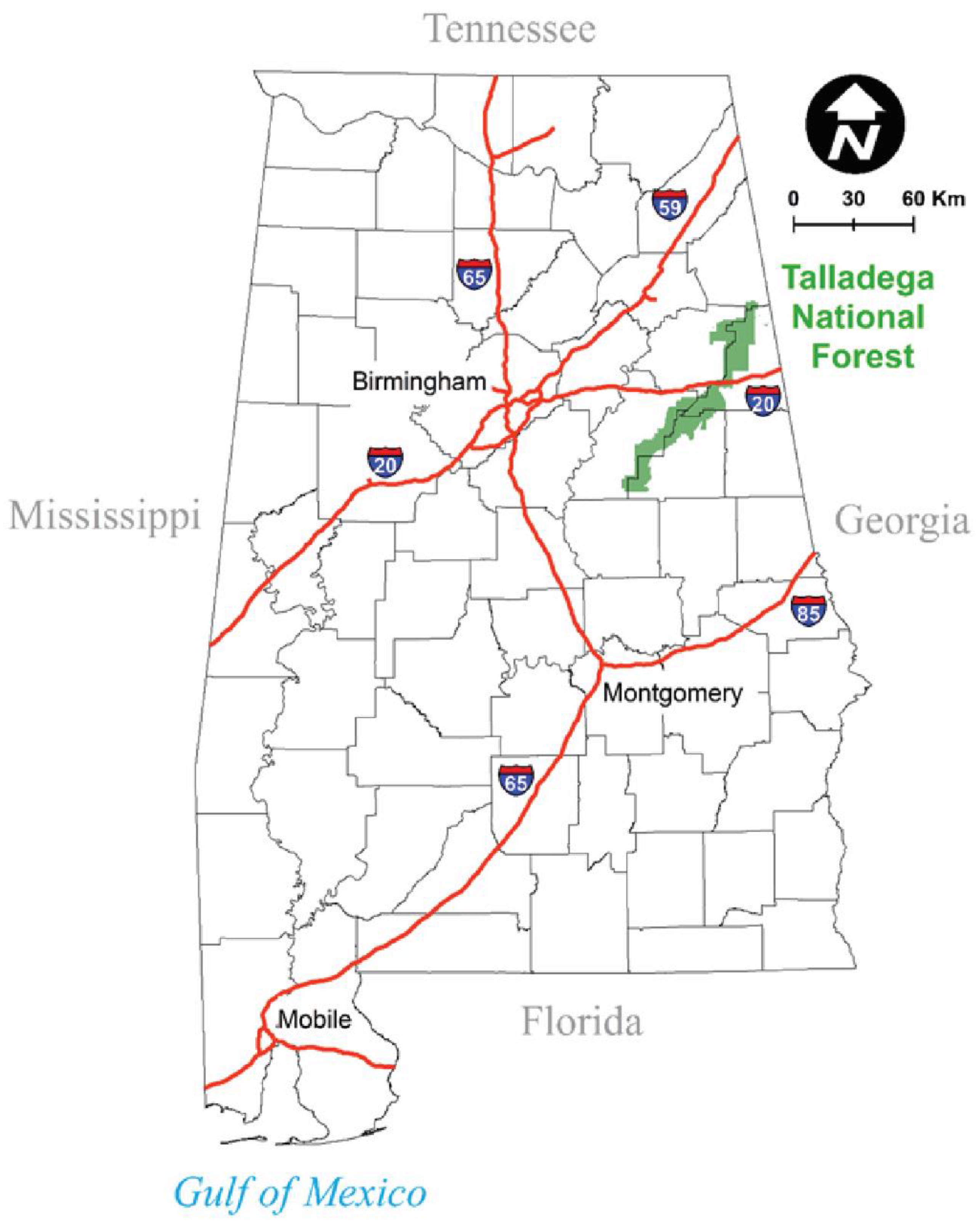
2.1. Study Area
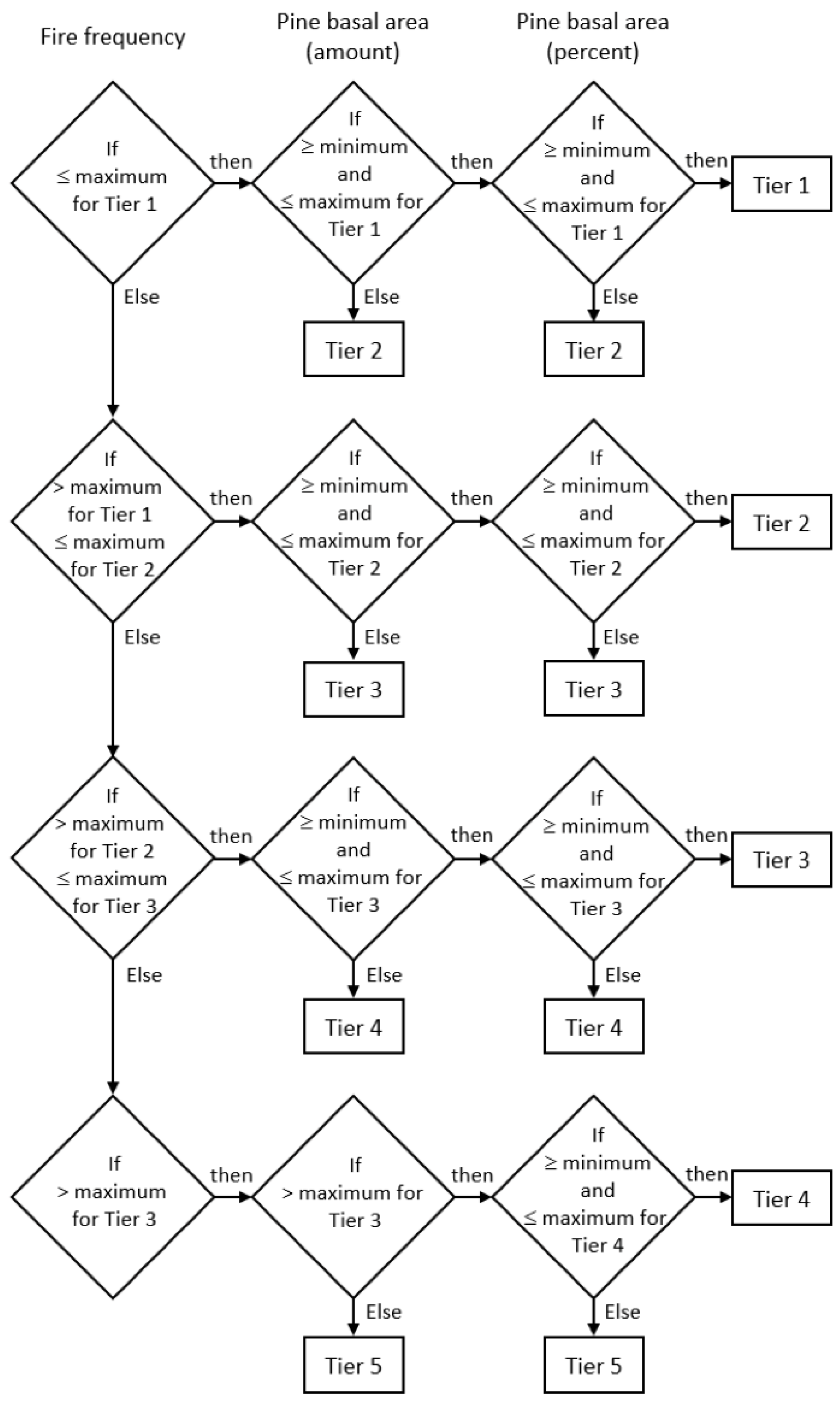
2.2. Analysis Methods
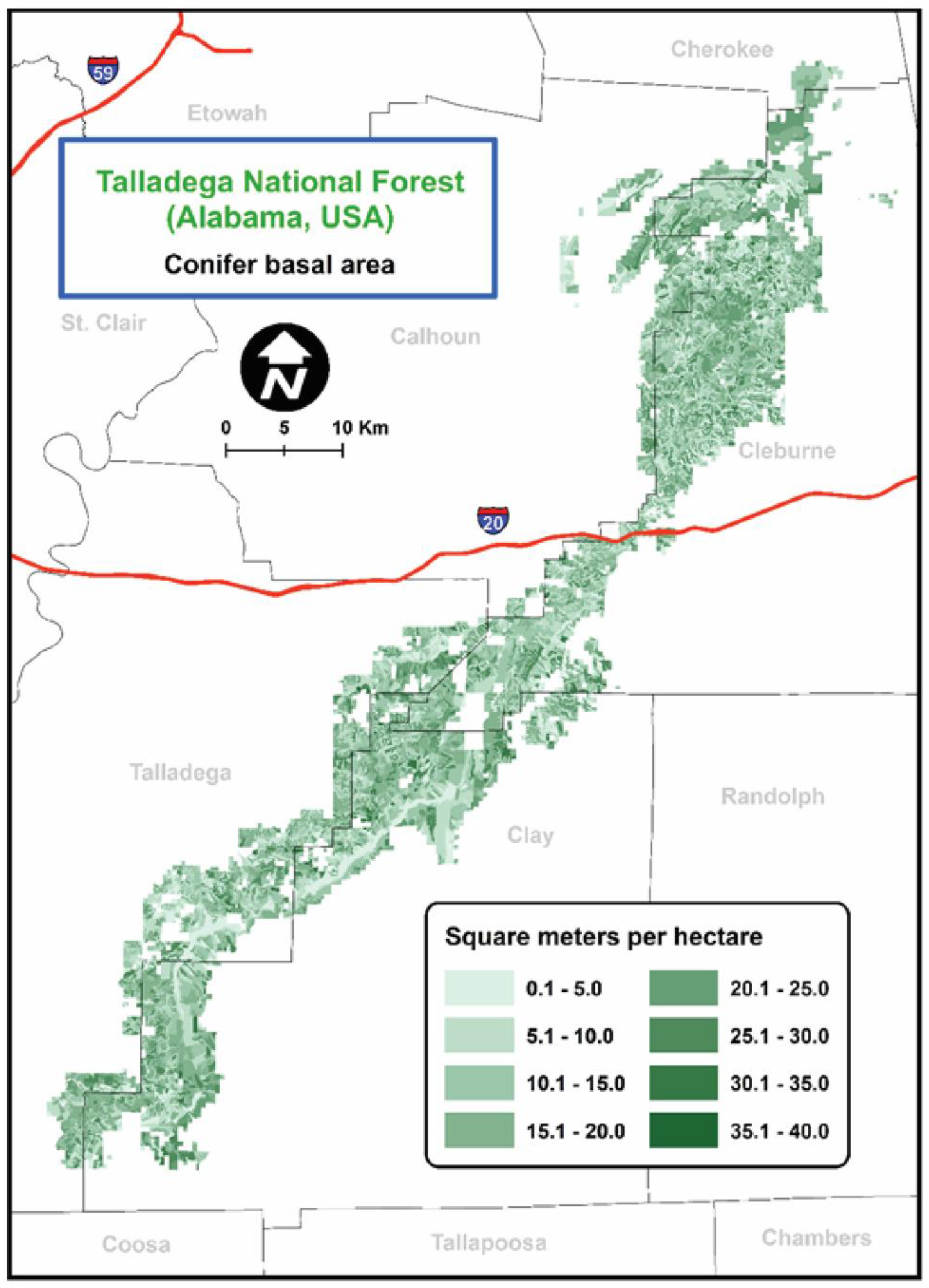
2.3. GIS Data
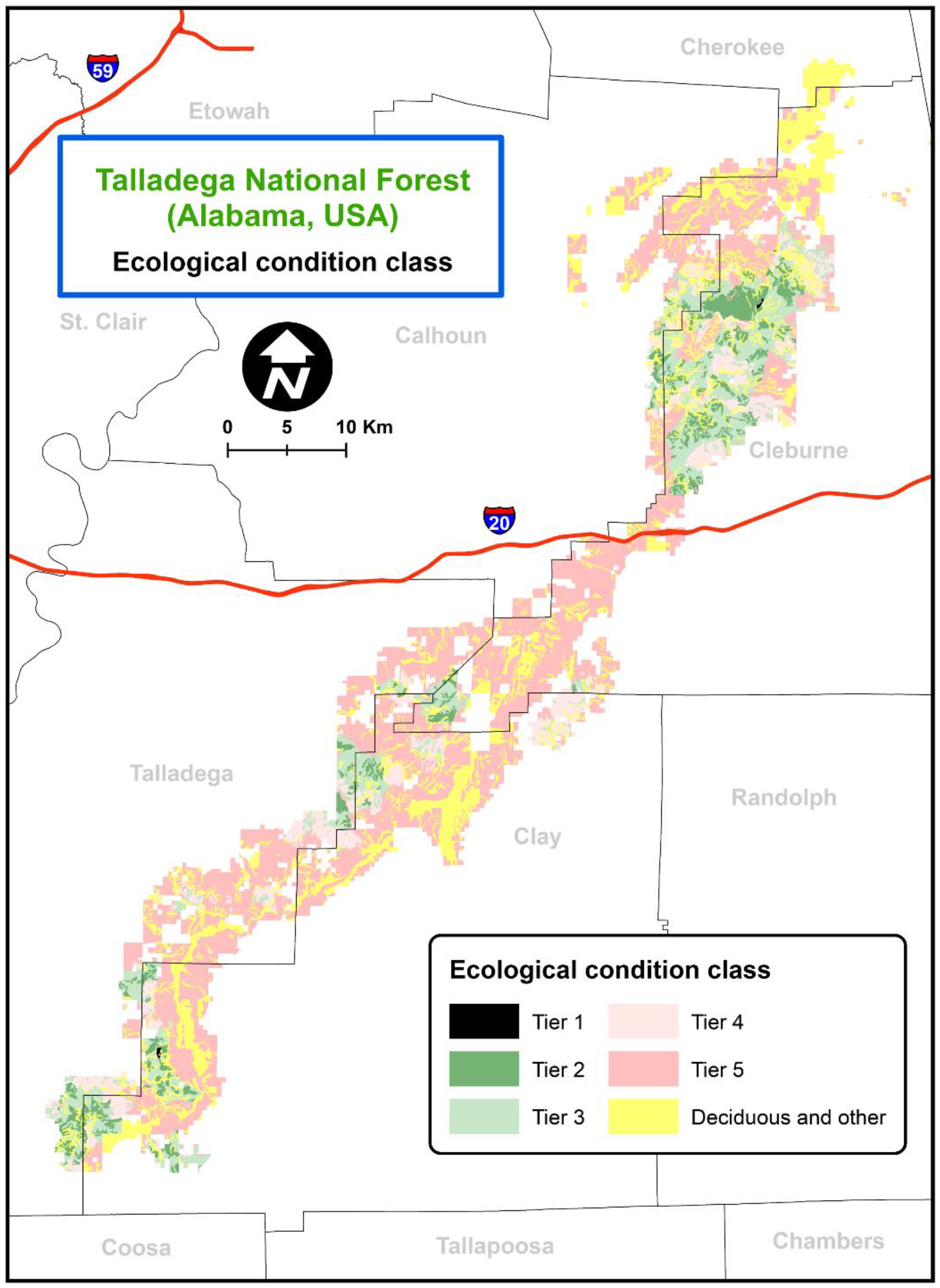
3. Results
4. Discussion
5. Conclusions
Author Contributions
Funding
Institutional Review Board Statement
Informed Consent Statement
Conflicts of Interest
References
- Waldrop, T.A.; Goodrick, S.L. Introduction to Prescribed Fires in Southern Ecosystems; Science Update SRS-054; U.S. Department of Agriculture, Forest Service, Southern Research Station: Asheville, NC, USA, 2018.
- Waldrop, T.A.; White, D.L.; Jones, S.M. Fire regimes for pine-grassland communities in the southeastern United States. For. Ecol. Manag. 1992, 47, 195–210. [Google Scholar] [CrossRef]
- Stambaugh, M.C.; Guyette, R.P.; Stroh, E.D.; Struckoff, M.A.; Whittier, J.B. Future southcentral US wildfire probability due to climate change. Clim. Chang. 2018, 147, 617–631. [Google Scholar] [CrossRef]
- Noss, R.F. Fire Ecology of Florida and the Southeastern Coastal Plain; University Press of Florida: Gainesville, FL, USA, 2018. [Google Scholar]
- Rentz, R. A brief history of reforestation and restoration in Louisiana. Tree Plant. Notes 2013, 56, 13–23. [Google Scholar]
- Bettinger, P.; Merry, K. Land cover transitions in the United States South: 2007–2013. Appl. Geogr. 2019, 105, 102–110. [Google Scholar] [CrossRef]
- U.S. Geological Survey. PAD-US Statistics and Reports, PAD-US 1.4 by State (US States and Territories) Protection Status Summary Statistics. Available online: https://www.usgs.gov/core-science-systems/science-analytics-and-synthesis/gap/science/pad-us-statistics-and-reports?qt-science_center_objects=0#qt-science_center_objects (accessed on 30 April 2022).
- Cleland, D.; Reynolds, K.; Vaughan, R.; Schrader, B.; Li, H.; Liang, L. Terrestrial condition assessment for national forests of the USDA Forest Service in the continental US. Sustainability 2017, 9, 2144. [Google Scholar] [CrossRef] [Green Version]
- Anderson, M.; Hayes, L.; Keyser, P.D.; Lituma, C.M.; Sutter, R.D.; Zollner, D. Shortleaf Pine Restoration Plan: Restoring an American Forest Legacy. Available online: https://shortleafpine.org/shortleaf-pine-initiative/shortleaf-pine-restoration-plan/shortleaf-pine-restoration-plan (accessed on 30 April 2002).
- Trager, M.D.; Drake, J.B.; Jenkins, A.M.; Petrick, C.J. Mapping and modeling ecological conditions of longleaf pine habitats in the Apalachicola National Forest. J. For. 2018, 116, 304–311. [Google Scholar] [CrossRef]
- Longleaf Partnership Council. America’s Longleaf Restoration Initiative, Strategic Priorities and Actions, 2019–2021. Available online: https://americaslongleaf.org/media/jvrle3tr/lpc-strategies-and-actions-2019.pdf (accessed on 30 April 2022).
- Martins, I.; Macedo, D.R.; Hughes, R.M.; Callisto, M. Are multiple multimetric indices effective for assessing ecological condition in tropical basins? Ecol. Indic. 2020, 110, 105953. [Google Scholar] [CrossRef]
- Evans, P.M.; Newton, A.C.; Cantarello, E.; Sanderson, N.; Jones, D.L.; Barsoum, N.; Cottrell, J.E.; A’Hara, S.W.; Fuller, L. Testing the relative sensitivity of 102 ecological variables as indicators of woodland condition in the New Forest, UK. Ecol. Indic. 2019, 107, 105575. [Google Scholar] [CrossRef]
- Constança Aguiar, F.; Rosário Fernandes, M.; Ferreira, M.T. Riparian vegetation metrics as tools for guiding ecological restoration in riverscapes. Knowl. Manag. Aquat. Ecosyst. 2011, 402, 21. [Google Scholar] [CrossRef]
- Kotze, D.C.; Ellery, W.N.; Macfarlane, W.N.; Jewitt, G.P.W. A rapid assessment method for coupling anthropogenic stressors and wetland ecological condition. Ecol. Indic. 2012, 13, 284–293. [Google Scholar] [CrossRef]
- Harwood, T.D.; Donohue, R.J.; Williams, K.J.; Ferrier, S.; McVicar, T.R.; Newell, G.; White, M. Habitat condition assess system: A new way to assess the condition of natural habitats for terrestrial biodiversity across whole regions using remote sensing data. Methods Ecol. Evol. 2016, 7, 1050–1059. [Google Scholar] [CrossRef]
- Goodridge Gaines, L.A.; Olds, A.D.; Henderson, C.J.; Connolly, R.M.; Schlacher, T.A.; Jones, T.R.; Gilby, B.L. Linking ecosystem condition and landscape context in the conservation of ecosystem multifunctionality. Biol. Conserv. 2020, 243, 108479. [Google Scholar] [CrossRef]
- Laughlin, D.C.; Strahan, R.T.; Huffman, D.W.; Sánchez Meador, A.J. Using trait-based ecology to restore resilient ecosystems: Historical conditions and the future of montane forests in western North America. Restor. Ecol. 2017, 25, S135–S146. [Google Scholar] [CrossRef]
- Cram, D.; Saud, P.; Baker, T. Structure and composition of a dry mixed-conifer forest in absence of contemporary treatments, Southwest, USA. Forests 2017, 8, 349. [Google Scholar] [CrossRef]
- Staus, N.L.; Strittholt, J.R.; Dellasala, D.A. Evaluating areas of high conservation value in western Oregon with a decision-support model. Conserv. Biol. 2010, 24, 711–720. [Google Scholar] [CrossRef]
- Hessburg, P.F.; Reynolds, K.M.; Salter, R.B.; Dickinson, J.D.; Gaines, W.L.; Harrod, R.J. Landscape evaluation for restoration planning on the Okanogan-Wenatchee National Forest, USA. Sustainability 2013, 5, 805–840. [Google Scholar] [CrossRef] [Green Version]
- Pechanec, V.; Brus, J.; Kilianová, H.; Machar, I. Decision support tool for the evaluation of landscapes. Ecol. Inform. 2015, 30, 305–308. [Google Scholar] [CrossRef]
- Sugumaran, R.; DeGroote, J. Spatial Decision Support Systems, Principles and Practices; CRC Press: Boca Raton, FL, USA, 2011. [Google Scholar]
- Bagstad, K.J.; Semmens, D.J.; Waage, S.; Winthrop, R. A comparative assessment of decision-support tools for ecosystem services quantification and valuation. Ecosyst. Serv. 2013, 5, e27–e39. [Google Scholar] [CrossRef]
- Stober, J.; Merry, K.; Bettinger, P. Analysis of fire frequency on the Talladega National Forest, USA, 1998–2018. Int. J. Wildland Fire 2020, 29, 919–925. [Google Scholar] [CrossRef]
- Varner, J.M., III; Kush, J.S.; Meldahl, R.S. Structural characteristics of frequently-burned old-growth longleaf pine stands in the mountains of Alabama. Castanea 2003, 68, 211–221. [Google Scholar]
- Shankman, D.; Wills, K.M., Jr. Pre-European settlement forest communities of the Talladega Mountains, Alabama. Southeast. Geog. 1995, 35, 118–131. [Google Scholar] [CrossRef]
- Weakley, A.S.; Evans, R.E. Pinus palustris—Pinus echinata/Quercus marilandica—(Quercus montana)/Vaccinium pallidum Woodland, CEGL003606. NatureServe Explorer: An Online Encyclopedia of Life. Available online: https://explorer.natureserve.org/Taxon/ELEMENT_GLOBAL.2.689504/Pinus_palustris_-_Pinus_echinata_-_Quercus_marilandica_-_(Quercus_montana)_-_Vaccinium_pallidum_Woodland (accessed on 30 April 2022).
- Weakley, A.S.; Govus, T. Pinus palustris—Pinus echinata—Quercus montana/Kalmia latifolia—Rhododendron minus Woodland. Available online: https://explorer.natureserve.org/Taxon/ELEMENT_GLOBAL.2.689459/Pinus_palustris_-_Pinus_echinata_-_Quercus_montana_-_Kalmia_latifolia_-_Rhododendron_minus_Woodland (accessed on 28 July 2015).
- Harper, R.M. Economic Botany of Alabama, Monograph 8, Part 1; Alabama Geological Survey: Tuscaloosa, AL, USA, 1913. [Google Scholar]
- Varner, J.M., III; Kush, J.S.; Meldahl, R.S. Vegetation of frequently-burned old-growth longleaf pine (Pinus palustris Mill.) savannas on Choccolocco Mountain, Alabama, USA. Nat. Areas J. 2003, 23, 43–52. [Google Scholar]
- Smith, G.C.; Patterson, M.W.; Trendell, H.R. The demise of the longleaf-pine ecosystem. Southeast. Geog. 2000, 40, 75–92. [Google Scholar] [CrossRef]
- U.S. Forest Service, Lands and Realty Management Staff. Establishment and Modification of National Forest Boundaries and National Grasslands. A Chronological Record 1891–2012; FS-612; U.S. Department of Agriculture, Forest Service, Lands and Realty Management Staff: Washington, DC, USA, 2012.
- Bale, A.M. Fire Effects and Litter Accumulation Dynamics in a Montane Longleaf Pine Ecosystem. Master’s Thesis, University of Missouri-Columbia, Columbia, MO, USA, 2009. [Google Scholar]
- Stambaugh, M.C.; Varner, J.M.; Jackson, S.T. Biogeography: An interweave of climate, fire, and humans. In Ecological Restoration and Management of Longleaf Pine Forests; Kirkman, K.L., Jack, S.B., Eds.; CRC Press: Boca Raton, FL, USA, 2018; pp. 17–38. [Google Scholar] [CrossRef]
- U.S. Forest Service. Revised Land and Resource Management Plan, National Forests in Alabama; Management Bulletin R8-MB 112A; U.S. Forest Service, Southern Region: Atlanta, GA, USA, 2004.
- Kirkman, L.K.; Jack, S.B. (Eds.) Ecological Restoration and Management of Longleaf Pine Forest; CRC Press: Boca Raton, FL, USA, 2018. [Google Scholar] [CrossRef]
- Rizzoli, A.E.; Young, W.J. Delivering environmental decision support systems: Software tools and techniques. Environ. Model. Softw. 1997, 12, 237–249. [Google Scholar] [CrossRef]
- Chang, K.-T. Introduction to Geographic Information Systems, 6th ed.; McGraw-Hill: New York, NY, USA, 2012. [Google Scholar]
- Hardisty, J.; Taylor, D.M.; Metcalf, S.E. Computerised Environmental Modelling, A Practical Introduction Using Excel; John Wiley & Sons: Chichester, UK, 1993. [Google Scholar]
- Hoang, T.H.; Mouton, A.; Lock, K.; De Pauw, N.; Goethals, P.L.M. Integrating data-driven ecological models in an expert-based decision support system for water management in the Du river basin (Vietnam). Environ. Monit. Assess. 2013, 185, 631–642. [Google Scholar] [CrossRef]
- Womack, B.; Carter, R. Landscape scale forest community classification in the Horseblock Mountain Region of the Talladega National Forest, Alabama. Nat. Areas J. 2011, 31, 51–64. [Google Scholar] [CrossRef]
- Mahan, C.G.; Young, J.A.; Miller, B.J.; Saunders, M.C. Using ecological indicators and a decision support system for integrated ecological assessment at two national park units in the Mid-Atlantic region, USA. Environ. Manag. 2015, 55, 508–522. [Google Scholar] [CrossRef] [Green Version]
- McNab, W.H. A topographic index to quantify the effect of mesoscale landform on site productivity. Can. J. For. Res. 1993, 23, 1100–1107. [Google Scholar] [CrossRef]
- Patterson, K.D.; White, R. Quercus montana—(Quercus coccinea)/Carya pallida/Vaccinium arboretum—Vaccinium pallidum Forest, CEGL008431. NatureServe Explorer: An Online Encyclopedia of Life. Available online: https://explorer.natureserve.org/Taxon/ELEMENT_GLOBAL.2.684808/Quercus_montana_-_(Quercus_coccinea)_-_Carya_pallida_-_Vaccinium_arboreum_-_Vaccinium_pallidum_Forest (accessed on 30 April 2022).
- Foody, G.M. Status of land cover classification accuracy assessment. Remote Sens. Environ. 2002, 80, 185–201. [Google Scholar] [CrossRef]
- Liu, C.; Frazier, P.; Kumar, L. Comparative assessment of the measures of thematic classification accuracy. Remote Sens. Environ. 2007, 107, 606–616. [Google Scholar] [CrossRef]
- Groffman, P.M.; Baron, J.S.; Blett, T.; Gold, A.J.; Goodman, I.; Gunderson, L.H.; Levinson, B.M.; Palmer, M.A.; Paerl, H.W.; Peterson, G.D.; et al. Ecological thresholds: The key to successful environmental management or an important concept with no practical application? Ecosystems 2006, 9, 1–13. [Google Scholar] [CrossRef]
- Reynolds, K.M.; Hessburg, P.F. Decision support for integrated landscape evaluation and restoration planning. For. Ecol. Manag. 2005, 207, 263–278. [Google Scholar] [CrossRef]
- Coops, N.C.; Tompalski, P.; Goodbody, T.R.H.; Achim, A.; Mulverhill, C. Framework for near real-time forest inventory using multi source remote sensing data. Forestry 2022, 2022, 1–19. [Google Scholar] [CrossRef]
- Luoma, V.; Vastaranta, M.; Eyvindson, K.; Kankare, V.; Saarinen, N.; Holopainen, M.; Hyyppä, J. Errors in the short-term forest resource information update. In The Rise of Big Spatial Data, Lecture Notes in Geoinformation and Cartography; Ivan, I., Singleton, A., Horák, J., Inspektor, T., Eds.; Springer: Cham, Switzerland, 2017; pp. 155–166. [Google Scholar] [CrossRef] [Green Version]
- Peters, S.; Liu, J.; Bruce, D.; Li, A.; Finn, A. Research note: Cost-efficient estimates of Pinus radiata wood volumes using multitemporal LiDAR data. Aust. For. 2021, 84, 206–214. [Google Scholar] [CrossRef]
- Bried, J.T.; Strout, K.L.; Portante, T. Coefficients of conservatism for the vascular flora of New York and New England: Inter-state comparisons and expert opinion bias. Northeast. Nat. 2012, 19, 101–114. [Google Scholar] [CrossRef]
- Cohen, M.J.; Carstenn, S.; Lane, C.R. Floristic quality indices for biotic assessment of depressional marsh condition in Florida. Ecol. Appl. 2004, 14, 784–794. [Google Scholar] [CrossRef] [Green Version]
- Hart, B.T.; Burgman, M.; Grace, M.; Pollino, C.; Thomas, C.; Webb, J.A. Risk-based approaches to managing contaminants in catchments. Hum. Ecol. Risk Assess. 2007, 12, 66–73. [Google Scholar] [CrossRef]
- Bettinger, P. Distributing geographic information systems capabilities to field offices: Benefits and challenges. J. For. 1999, 97, 22–26. [Google Scholar] [CrossRef]


| Tier | Minimum Pine Basal Area (m2/ha) | Maximum Pine Basal Area (m2/ha) | Minimum Pine Basal Area (%) | Maximum Pine Basal Area (%) | Maximum Fire Return Interval (years) |
|---|---|---|---|---|---|
| 1 | 9.2 | 18.4 | 80 | 100 | 3 |
| 2 | 11.5 | 18.4 | 60 | 80 | 5 |
| 3 | 18.4 | 27.6 | 40 | 60 | 7 |
| 4 | 27.6 | --- | 20 | 40 | >7 |
| 5 | --- | 27.6 | --- | --- | >7 |
| Modeled | Reference Tier (Expert Opinion) | User’s | |||||
|---|---|---|---|---|---|---|---|
| Tier | 1 | 2 | 3 | 4 | 5 | Total | Accuracy (%) |
| 1 | 1 | 0 | 0 | 0 | 0 | 1 | 100.00 |
| 2 | 11 | 23 | 8 | 5 | 0 | 47 | 48.9 |
| 3 | 9 | 14 | 10 | 4 | 1 | 38 | 26.3 |
| 4 | 0 | 5 | 12 | 10 | 0 | 27 | 37.0 |
| 5 | 0 | 2 | 5 | 20 | 33 | 60 | 55.0 |
| Total | 21 | 44 | 35 | 39 | 34 | 173 | |
| Producer’s Accuracy (%) | 4.8 | 52.3 | 28.6 | 25.6 | 97.1 | ||
| Modeled | Reference Tier (Expert Opinion) | User’s | |||||
|---|---|---|---|---|---|---|---|
| Tier | 1 | 2 | 3 | 4 | 5 | Total | Accuracy (%) |
| 1 | 1 | 0 | 0 | 0 | 0 | 1 | 100.00 |
| 2 | 11 | 23 | 8 | 5 | 0 | 47 | 89.4 |
| 3 | 9 | 14 | 10 | 4 | 1 | 38 | 73.7 |
| 4 | 0 | 5 | 12 | 10 | 0 | 27 | 81.5 |
| 5 | 0 | 2 | 5 | 20 | 33 | 60 | 88.3 |
| Total | 21 | 44 | 35 | 39 | 34 | 173 | |
| Producer’s Accuracy (%) | 57.1 | 84.1 | 85.7 | 87.2 | 97.1 | ||
Publisher’s Note: MDPI stays neutral with regard to jurisdictional claims in published maps and institutional affiliations. |
© 2022 by the authors. Licensee MDPI, Basel, Switzerland. This article is an open access article distributed under the terms and conditions of the Creative Commons Attribution (CC BY) license (https://creativecommons.org/licenses/by/4.0/).
Share and Cite
Bettinger, P.; Merry, K.; Stober, J. A Hierarchical Binary Process Model to Assess Deviation from Desired Ecological Condition across a Broad Forested Landscape in Alabama. Land 2022, 11, 775. https://doi.org/10.3390/land11060775
Bettinger P, Merry K, Stober J. A Hierarchical Binary Process Model to Assess Deviation from Desired Ecological Condition across a Broad Forested Landscape in Alabama. Land. 2022; 11(6):775. https://doi.org/10.3390/land11060775
Chicago/Turabian StyleBettinger, Pete, Krista Merry, and Jonathan Stober. 2022. "A Hierarchical Binary Process Model to Assess Deviation from Desired Ecological Condition across a Broad Forested Landscape in Alabama" Land 11, no. 6: 775. https://doi.org/10.3390/land11060775
APA StyleBettinger, P., Merry, K., & Stober, J. (2022). A Hierarchical Binary Process Model to Assess Deviation from Desired Ecological Condition across a Broad Forested Landscape in Alabama. Land, 11(6), 775. https://doi.org/10.3390/land11060775