
How Eco-Efficiency Is the Forestry Ecological Restoration Program? The Case of the Sloping Land Conversion Program in the Loess Plateau, China

 ,
,  ,
,  ,
,
Abstract
:1. Introduction
2. Materials and Methods
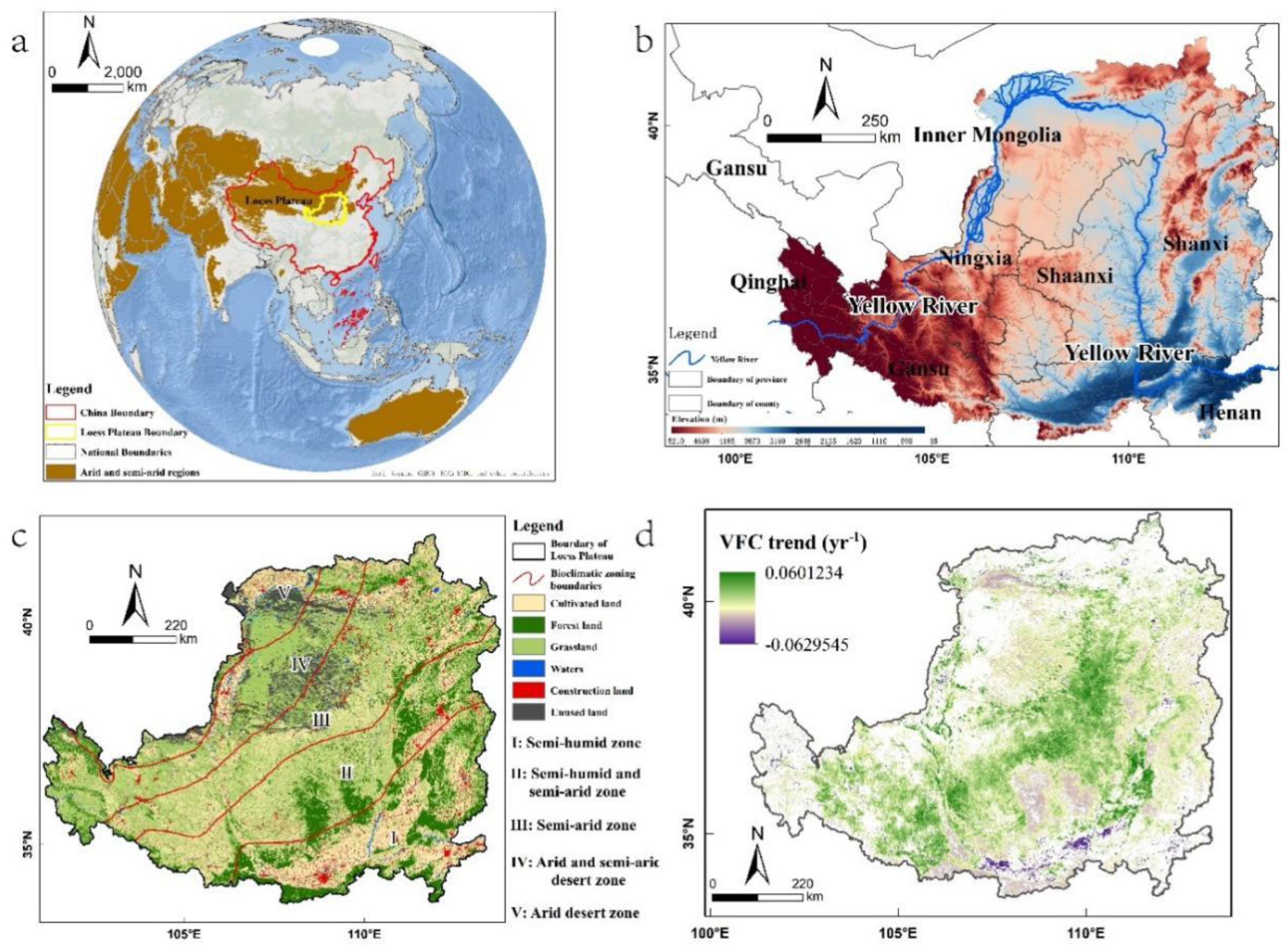
2.1. Study Area
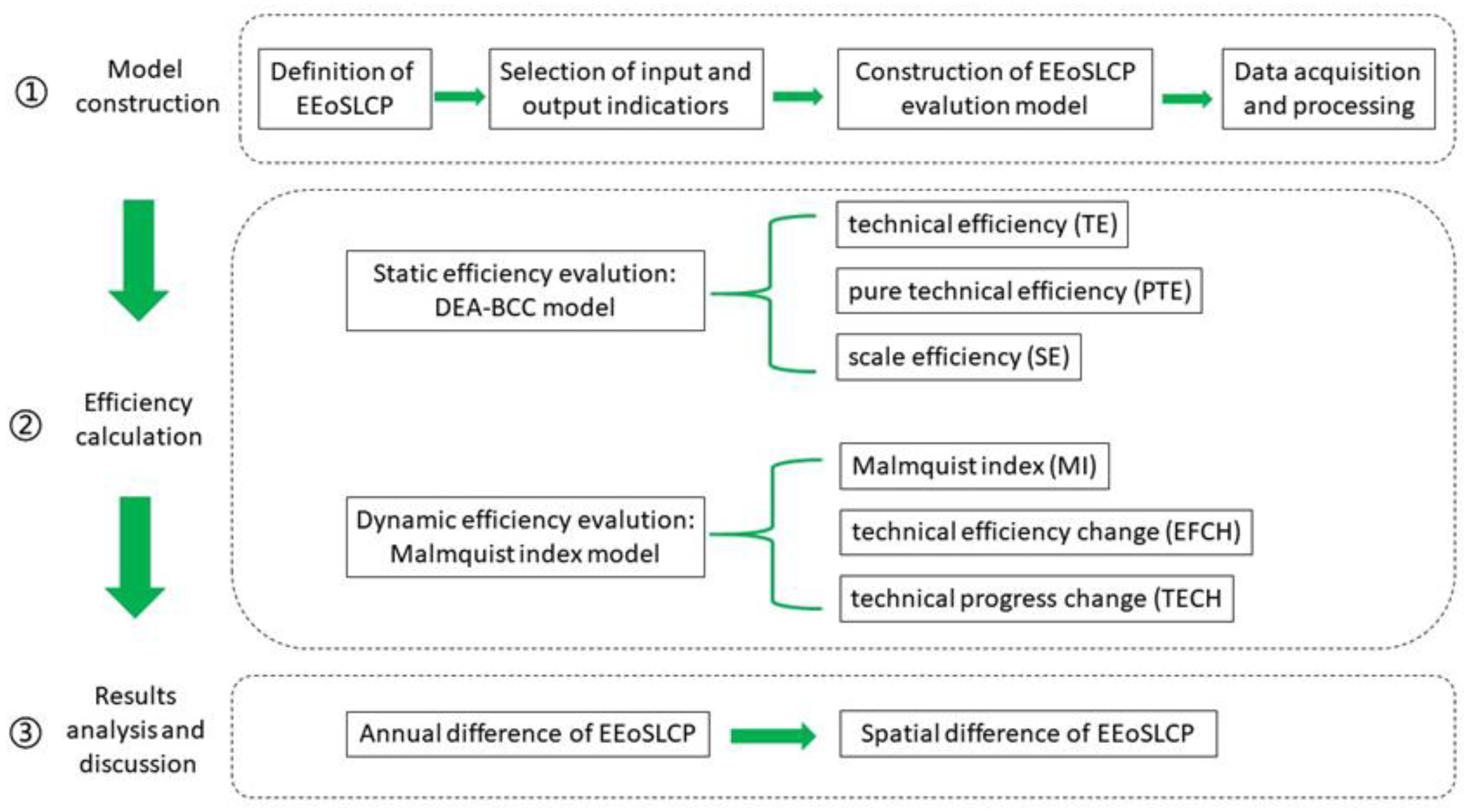
2.2. Methodology
2.3. Definition of EEoFERP
2.3.1. Input Indexes of EEoFERP
2.3.2. Output Indexes of EEoFERP
2.4. Methods
2.4.1. Ecological Effects Calculation of SLCP
2.4.2. DEA Model
2.4.3. Malmquist Index Model
2.5. Data Sources
3. Results
3.1. Static Efficiency Based on DEA–BCC Model
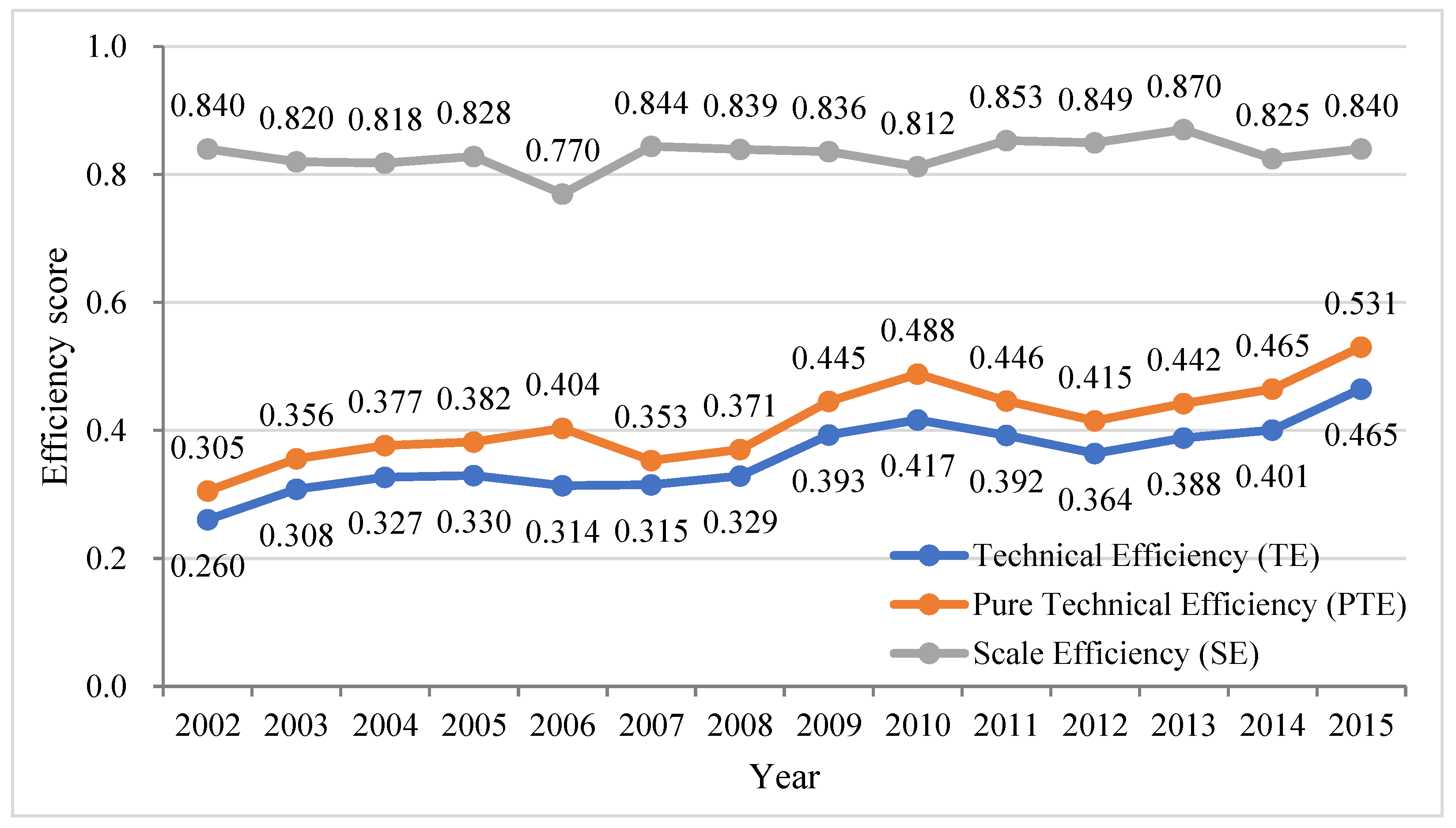
3.1.1. The Annual Difference in Static Efficiency
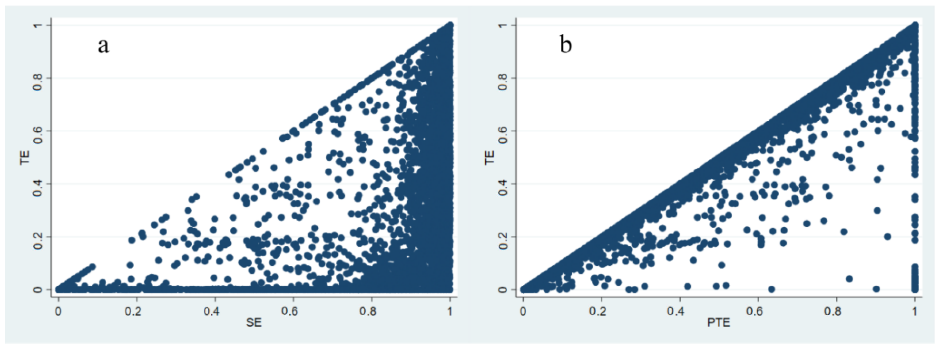
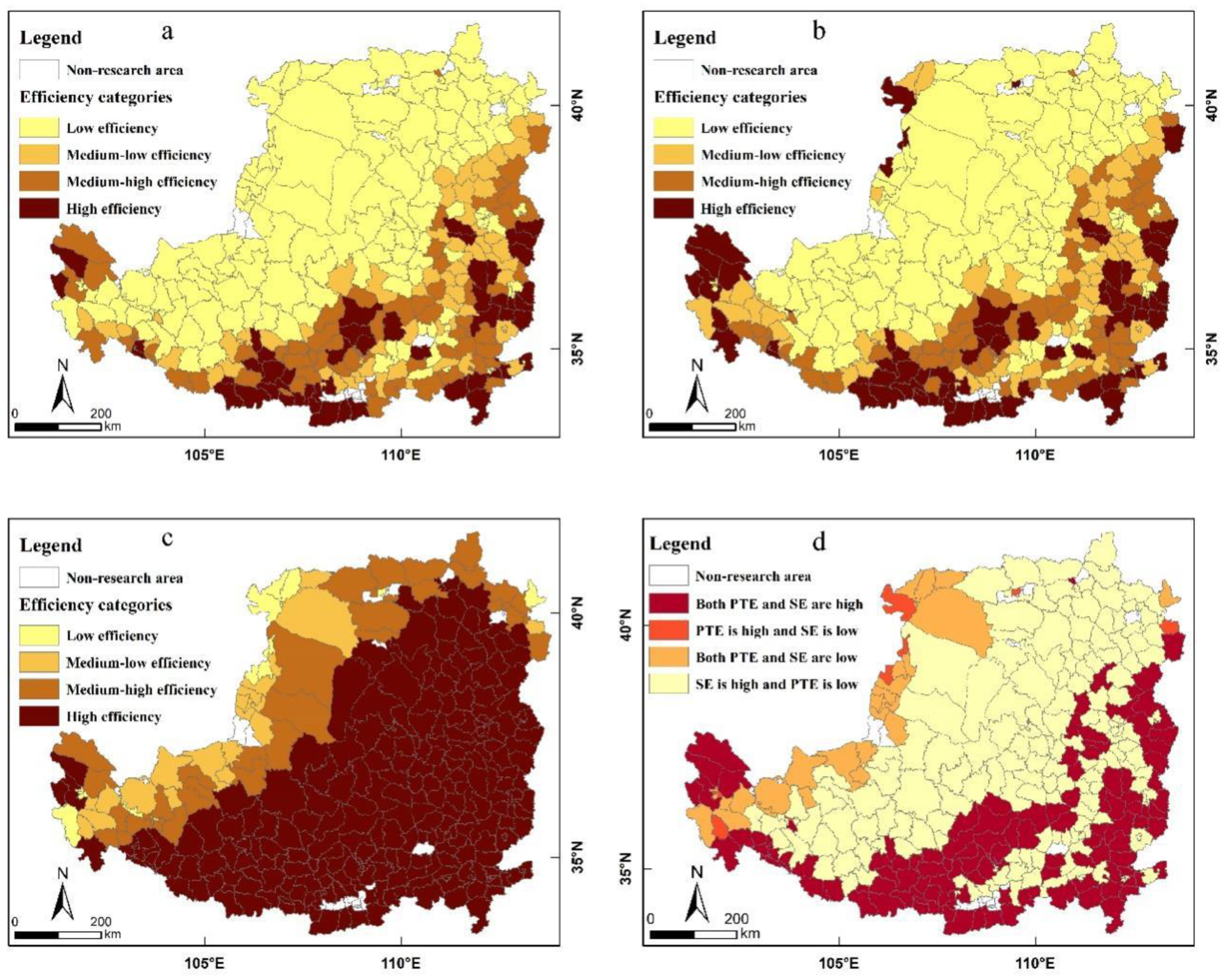
3.1.2. County Difference in Static Efficiency
3.2. Dynamic Efficiency Based on the Malmquist Index Method
3.2.1. The Annual Difference in Dynamic Efficiency
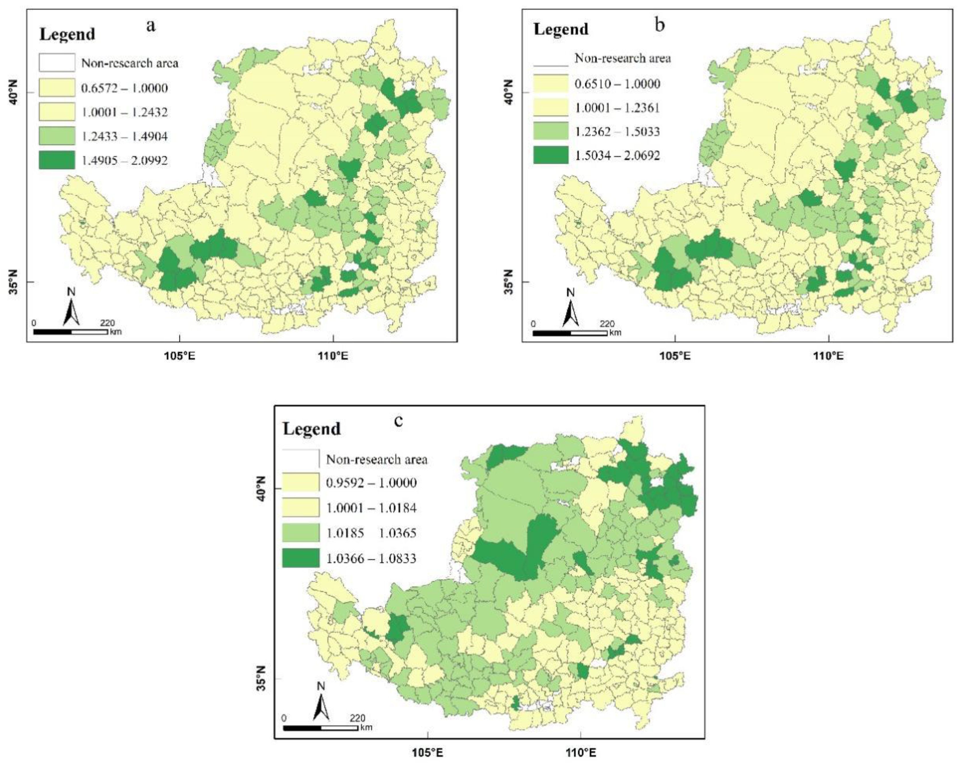
3.2.2. County Difference in Dynamic Efficiency
4. Discussion
5. Conclusions and Policy Implications
5.1. Conclusions
5.2. Policy Implications
Supplementary Materials
Author Contributions
Funding
Data Availability Statement
Acknowledgments
Conflicts of Interest
References
- Dao, H.; Peduzzi, P.; Friot, D. National Environmental Limits and Footprints Based on the Planetary Boundaries Framework: The Case of Switzerland. Glob. Environ. Chang. 2018, 52, 49–57. [Google Scholar] [CrossRef] [Green Version]
- Millennium Ecosystem Assessment. Ecosystems and Human Well-Being; Island Press: Washington, DC, USA, 2005. [Google Scholar]
- Mbow, H.-O.P.; Reisinger, A.; Canadell, J.; O’Brien, P. Special Report on Climate Change, Desertification, Land Degradation, Sustainable Land Management, Food Security, and Greenhouse Gas Fluxes in Terrestrial Ecosystems (SR2); IPCC: Ginevra, Switzerland, 2017; Volume 650. [Google Scholar]
- Georgescu-Roegen, N. The Entropy Law and the Economic Process. In The Entropy Law and the Economic Process; Harvard University Press: Cambridge, CA, USA, 2013. [Google Scholar]
- Georgescu-Roegen, N. Energy Analysis and Economic Valuation. South. Econ. J. 1979, 45, 1023–1058. [Google Scholar] [CrossRef]
- Meadows, D.H.; Meadows, D.H.; Randers, J.; Behrens, W.W., III. The Limits to Growth: A Report to the Club of Rome (1972). Google Sch. 1972, 91. [Google Scholar]
- Daly, H.E.; Farley, J. Ecological Economics: Principles and Applications; Island Press: Washington, DC, USA, 2011. [Google Scholar]
- Waltham, N.J.; Elliott, M.; Lee, S.Y.; Lovelock, C.; Duarte, C.M.; Buelow, C.; Simenstad, C.; Nagelkerken, I.; Claassens, L.; Wen, C.K.-C.; et al. UN Decade on Ecosystem Restoration 2021–2030—What Chance for Success in Restoring Coastal Ecosystems? Front. Mar. Sci. 2020, 7, 71. [Google Scholar] [CrossRef] [Green Version]
- Dahl, J. Progress and Development of the Prairie States Forestry Project. J. For. 1940, 38, 301–306. [Google Scholar] [CrossRef]
- Darier, É. Environmental Governmentality: The Case of Canada’s Green Plan. Environ. Politics 1996, 5, 585–606. [Google Scholar] [CrossRef]
- Mirzabaev, A.; Sacande, M.; Motlagh, F.; Shyrokaya, A.; Martucci, A. Economic Efficiency and Targeting of the African Great Green Wall. Nat. Sustain. 2022, 5, 17–25. [Google Scholar] [CrossRef]
- Resosudarmo, B.P. The Politics and Economics of Indonesia’s Natural Resources; ISEAS Publishing: Singapore, 2005; ISBN 978-981-230-549-7. [Google Scholar]
- Park, M.S.; Lee, H. Forest Policy and Law for Sustainability within the Korean Peninsula. Sustainability 2014, 6, 5162–5186. [Google Scholar] [CrossRef] [Green Version]
- Wil, D.J.; Do, D.S.; Trieu, V.H. Forest Rehabilitation in Vietnam: Histories, Realities and Future; Center for International Forestry Research (CIFOR): Bogor, Indonesia, 2006; ISBN 978-979-24-4652-4. [Google Scholar]
- Bryan, B.A.; Gao, L.; Ye, Y.; Sun, X.; Connor, J.D.; Crossman, N.D.; Stafford-Smith, M.; Wu, J.; He, C.; Yu, D.; et al. China’s Response to a National Land-System Sustainability Emergency. Nature 2018, 559, 193–204. [Google Scholar] [CrossRef]
- Lu, G.; Yin, R. Evaluating the Evaluated Socioeconomic Impacts of China’s Sloping Land Conversion Program. Ecol. Econ. 2020, 177, 106785. [Google Scholar] [CrossRef]
- Chen, C.; Park, T.; Wang, X.; Piao, S.; Xu, B.; Chaturvedi, R.K.; Fuchs, R.; Brovkin, V.; Ciais, P.; Fensholt, R.; et al. China and India Lead in Greening of the World through Land-Use Management. Nat. Sustain. 2019, 2, 122–129. [Google Scholar] [CrossRef] [PubMed]
- Qiu, S.; Peng, J.; Zheng, H.; Xu, Z.; Meersmans, J. How Can Massive Ecological Restoration Programs Interplay with Social-Ecological Systems? A Review of Research in the South China Karst Region. Sci. Total Environ. 2022, 807, 150723. [Google Scholar] [CrossRef] [PubMed]
- Countries Commit to Restore Global Land Area the Size of China. Available online: http://www.unep.org/news-and-stories/story/countries-commit-restore-global-land-area-size-china (accessed on 10 April 2022).
- Restoration Call for Area ‘the Size of China’ to Protect Falling Biodiversity and Food Insecurity. Available online: https://news.un.org/en/story/2021/06/1093272 (accessed on 10 April 2022).
- Birch, J.C.; Newton, A.C.; Aquino, C.A.; Cantarello, E.; Echeverría, C.; Kitzberger, T.; Schiappacasse, I.; Garavito, N.T. Cost-Effectiveness of Dryland Forest Restoration Evaluated by Spatial Analysis of Ecosystem Services. Proc. Natl. Acad. Sci. USA 2010, 107, 21925–21930. [Google Scholar] [CrossRef] [PubMed] [Green Version]
- Molin, P.G.; Chazdon, R.; Frosini de Barros Ferraz, S.; Brancalion, P.H.S. A Landscape Approach for Cost-Effective Large-Scale Forest Restoration. J. Appl. Ecol. 2018, 55, 2767–2778. [Google Scholar] [CrossRef]
- Schiappacasse, I.; Nahuelhual, L.; Vásquez, F.; Echeverría, C. Assessing the Benefits and Costs of Dryland Forest Restoration in Central Chile. J. Environ. Manag. 2012, 97, 38–45. [Google Scholar] [CrossRef]
- Newton, A.C.; del Castillo, R.F.; Echeverría, C.; Geneletti, D.; González-Espinosa, M.; Malizia, L.R.; Premoli, A.C.; Benayas, J.M.R.; Smith-Ramírez, C.; Williams-Linera, G. Forest Landscape Restoration in the Drylands of Latin America. Ecol. Soc. 2012, 17, 1. [Google Scholar] [CrossRef] [Green Version]
- Wang, X.; Bennett, J. Policy Analysis of the Conversion of Cropland to Forest and Grassland Program in China. Environ. Econ. Policy Stud. 2008, 9, 119–143. [Google Scholar] [CrossRef]
- Xian, J.; Xia, C.; Cao, S. Cost–Benefit Analysis for China’s Grain for Green Program. Ecol. Eng. 2020, 151, 105850. [Google Scholar] [CrossRef]
- Li, K.; Hou, Y.; Andersen, P.S.; Xin, R.; Rong, Y.; Skov-Petersen, H. Identifying the Potential Areas of Afforestation Projects Using Cost-Benefit Analysis Based on Ecosystem Services and Farmland Suitability: A Case Study of the Grain for Green Project in Jinan, China. Sci. Total Environ. 2021, 787, 147542. [Google Scholar] [CrossRef]
- Neto, J.Q.F.; Walther, G.; Bloemhof, J.; Van Nunen, J.; Spengler, T. A Methodology for Assessing Eco-Efficiency in Logistics Networks. Eur. J. Oper. Res. 2009, 193, 670–682. [Google Scholar] [CrossRef] [Green Version]
- Wang, Y.; Zhang, T.; Yao, S.; Deng, Y. Spatio-Temporal Evolution and Factors Influencing the Control Efficiency for Soil and Water Loss in the Wei River Catchment, China. Sustainability 2019, 11, 216. [Google Scholar] [CrossRef] [Green Version]
- Wu, X.; Wang, S.; Fu, B.; Liu, J. Spatial Variation and Influencing Factors of the Effectiveness of Afforestation in China’s Loess Plateau. Sci. Total Environ. 2021, 771, 144904. [Google Scholar] [CrossRef] [PubMed]
- Zhang, Y.; Zhang, D. Efficiency Measurement and Influencing Factors of Ecological Compensation: A Case Study from Wuqi and Zhidan on the Loess Plateau. Nat. Resour. Res. 2021, 30, 4905–4921. [Google Scholar] [CrossRef]
- Li, G.; Sun, S.; Han, J.; Yan, J.; Liu, W.; Wei, Y.; Lu, N.; Sun, Y. Impacts of Chinese Grain for Green Program and Climate Change on Vegetation in the Loess Plateau during 1982–2015. Sci. Total Environ. 2019, 660, 177–187. [Google Scholar] [CrossRef]
- Wu, X.; Wei, Y.; Fu, B.; Wang, S.; Zhao, Y.; Moran, E.F. Evolution and Effects of the Social-Ecological System over a Millennium in China’s Loess Plateau. Sci. Adv. 2020, 6, eabc0276. [Google Scholar] [CrossRef] [PubMed]
- Zhao, G.; Mu, X.; Wen, Z.; Wang, F.; Gao, P. Soil Erosion, Conservation, and Eco-Environment Changes in the Loess Plateau of China. Land Degrad. Dev. 2013, 24, 499–510. [Google Scholar] [CrossRef]
- Chen, Y.; Wang, K.; Lin, Y.; Shi, W.; Song, Y.; He, X. Balancing Green and Grain Trade. Nature Geosci. 2015, 8, 739–741. [Google Scholar] [CrossRef]
- Wang, S.; Zhao, D.; Chen, H. Government Corruption, Resource Misallocation, and Ecological Efficiency. Energy Econ. 2020, 85, 104573. [Google Scholar] [CrossRef]
- Amacher, G.S.; Ollikainen, M.; Koskela, E. Economics of Forest Resources; Mit Press Cambridge: Cambridge, CA, USA, 2009. [Google Scholar]
- He, L.; Guo, J.; Jiang, Q.; Zhang, Z.; Yu, S. How Did the Chinese Loess Plateau Turn Green from 2001 to 2020? An Explanation Using Satellite Data. Catena 2022, 214, 106246. [Google Scholar] [CrossRef]
- Jin, F.; Yang, W.; Fu, J.; Li, Z. Effects of Vegetation and Climate on the Changes of Soil Erosion in the Loess Plateau of China. Sci. Total Environ. 2021, 773, 145514. [Google Scholar] [CrossRef]
- Li, J.; Peng, S.; Li, Z. Detecting and Attributing Vegetation Changes on China’s Loess Plateau. Agric. For. Meteorol. 2017, 247, 260–270. [Google Scholar] [CrossRef]
- Zhang, D.; Pearse, P.H. Forest Economics; UBC Press: Vancouve, BC, Canada, 2011. [Google Scholar]
- Li, J.; Wang, X.; Shao, M.; Zhao, Y.; Li, X.; Wu, S.; Li, J.; Zhang, R. Simulation of Biomass and Soil Desiccation of Robinia Pseudoacacia Forestlands on Semi-Arid and Semi-Humid Regions of China’s Loess Plateau. Chin. J. Plant Ecol. 2010, 34, 330–339. [Google Scholar] [CrossRef]
- Qian, C.; Shao, L.; Hou, X.; Zhang, B.; Chen, W.; Xia, X. Detection and Attribution of Vegetation Greening Trend across Distinct Local Landscapes under China’s Grain to Green Program: A Case Study in Shaanxi Province. Catena 2019, 183, 104182. [Google Scholar] [CrossRef]
- Deng, L.; Liu, S.; Kim, D.G.; Peng, C.; Sweeney, S.; Shangguan, Z. Past and Future Carbon Sequestration Benefits of China’s Grain for Green Program. Glob. Environ. Chang. 2017, 47, 13–20. [Google Scholar] [CrossRef]
- Feng, X.; Fu, B.; Lu, N.; Zeng, Y.; Wu, B. How Ecological Restoration Alters Ecosystem Services: An Analysis of Carbon Sequestration in China’s Loess Plateau. Sci. Rep. 2013, 3, 2846. [Google Scholar] [CrossRef]
- Wang, Y.; Zhao, J.; Fu, J.; Wei, W. Effects of the Grain for Green Program on the Water Ecosystem Services in an Arid Area of China-Using the Shiyang River Basin as an Example. Ecol. Indic. 2019, 104, 659–668. [Google Scholar] [CrossRef]
- Hua, F.; Wang, X.; Zheng, X.; Fisher, B.; Wang, L.; Zhu, J.; Tang, Y.; Yu, D.W.; Wilcove, D.S. Opportunities for Biodiversity Gains under the World’s Largest Reforestation Programme. Nat. Commun. 2016, 7, 12717. [Google Scholar] [CrossRef] [Green Version]
- Wang, F.; Pan, X.; Gerlein-Safdi, C.; Cao, X.; Wang, S.; Gu, L.; Wang, D.; Lu, Q. Vegetation Restoration in Northern China: A Contrasted Picture. Land Degrad. Dev. 2020, 31, 669–676. [Google Scholar] [CrossRef]
- Chen, J.; Fan, W.; Li, D.; Liu, X.; Song, M. Driving Factors of Global Carbon Footprint Pressure: Based on Vegetation Carbon Sequestration. Appl. Energy 2020, 267, 114914. [Google Scholar] [CrossRef]
- Peng, S.; Wen, D.; He, N.; Yu, G.; Ma, A.; Wang, Q. Carbon Storage in China’s Forest Ecosystems: Estimation by Different Integrative Methods. Ecol. Evol. 2016, 6, 3129–3145. [Google Scholar] [CrossRef] [Green Version]
- Xu, L.; Yu, G.; He, N.; Wang, Q.; Gao, Y.; Wen, D.; Li, S.; Niu, S.; Ge, J. Carbon Storage in China’s Terrestrial Ecosystems: A Synthesis. Sci. Rep. 2018, 8, 2806. [Google Scholar] [CrossRef] [PubMed]
- Xu, L.; He, N.; Yu, G. A Dataset of Carbon Density in Chinese Terrestrial Ecosystems (2010s); Science Data Bank: Beijing, China, 29 July 2018. [Google Scholar] [CrossRef]
- Renard, K.G. Predicting Soil Erosion by Water: A Guide to Conservation Planning with the Revised Universal Soil Loss Equation (RUSLE); United States Government Printing: Washington, DC, USA, 1997.
- Wischmeier, W.H.; Smith, D.D. Predicting Rainfall Erosion Losses: A Guide to Conservation Planning; Department of Agriculture, Science and Education Administration: Washington, DC, USA, 1978.
- Williams, J.R.; Renard, K.G.; Dyke, P.T. EPIC: A New Method for Assessing Erosion’s Effect on Soil Productivity. J. Soil Water Conserv. 1983, 38, 381–383. [Google Scholar]
- Zhang, H.; Yang, Q.; Li, R.; Liu, Q.; Moore, D.; He, P.; Ritsema, C.J.; Geissen, V. Extension of a GIS Procedure for Calculating the RUSLE Equation LS Factor. Comput. Geosci. 2013, 52, 177–188. [Google Scholar] [CrossRef]
- Cai, C.; Ding, S.; Shi, Z.; Huang, L.; Zhang, G. Study of applying USLE and geographical information system IDRISI to predict soil erosion in small watershed. J. Soil Water Conserv. 2000, 14, 19–24. [Google Scholar]
- Yan, R.; Zhang, X.; Yan, S.; Chen, H. Estimating Soil Erosion Response to Land Use/Cover Change in a Catchment of the Loess Plateau, China. Int. Soil Water Conserv. Res. 2018, 6, 13–22. [Google Scholar] [CrossRef]
- Wu, X.; Wang, S.; Fu, B.; Liu, Y.; Zhu, Y. Land Use Optimization Based on Ecosystem Service Assessment: A Case Study in the Yanhe Watershed. Land Use Policy 2018, 72, 303–312. [Google Scholar] [CrossRef]
- Kong, L.; Zheng, H.; Rao, E.; Xiao, Y.; Ouyang, Z.; Li, C. Evaluating Indirect and Direct Effects of Eco-Restoration Policy on Soil Conservation Service in Yangtze River Basin. Sci. Total Environ. 2018, 631–632, 887–894. [Google Scholar] [CrossRef]
- Liu, W.; Liu, J.; Kuang, W. Spatiotemporal patterns of soil protection effect of the Grain for Green Project in northern Shaanxi. Acta Geogr. Sin. 2019, 74, 1835–1852. [Google Scholar]
- Carreño, L.; Frank, F.C.; Viglizzo, E.F. Tradeoffs between Economic and Ecosystem Services in Argentina during 50 Years of Land-Use Change. Agric. Ecosyst. Environ. 2012, 154, 68–77. [Google Scholar] [CrossRef]
- Liu, Y.; Lü, Y.; Jiang, W.; Zhao, M. Mapping Critical Natural Capital at a Regional Scale: Spatiotemporal Variations and the Effectiveness of Priority Conservation. Environ. Res. Lett. 2020, 15, 124025. [Google Scholar] [CrossRef]
- Duan, Y.; Di, B.; Ustin, S.L.; Xu, C.; Xie, Q.; Wu, S.; Li, J.; Zhang, R. Changes in Ecosystem Services in a Montane Landscape Impacted by Major Earthquakes: A Case Study in Wenchuan Earthquake-Affected Area, China. Ecol. Indic. 2021, 126, 107683. [Google Scholar] [CrossRef]
- Barral, M.P.; Oscar, M.N. Land-Use Planning Based on Ecosystem Service Assessment: A Case Study in the Southeast Pampas of Argentina. Agric. Ecosyst. Environ. 2012, 154, 34–43. [Google Scholar] [CrossRef]
- Charnes, A.; Cooper, W.W.; Rhodes, E. Measuring the Efficiency of Decision Making Units. Eur. J. Oper. Res. 1978, 2, 429–444. [Google Scholar] [CrossRef]
- Farrell, M.J. The Measurement of Productive Efficiency. J. R. Stat. Soc. Ser. A Gen. 1957, 120, 253–281. [Google Scholar] [CrossRef]
- Banker, R.D.; Charnes, A.; Cooper, W.W. Some Models for Estimating Technical and Scale Inefficiencies in Data Envelopment Analysis. Manag. Sci. 1984, 30, 1078–1092. [Google Scholar] [CrossRef] [Green Version]
- Färe, R.; Grosskopf, S.; Norris, M.; Zhang, Z. Productivity Growth, Technical Progress, and Efficiency Change in Industrialized Countries. Am. Econ. Rev. 1994, 84, 66–83. [Google Scholar]
- Malmquist, S. Index Numbers and Indifference Surfaces. Trab. Estad. 1953, 4, 209–242. [Google Scholar] [CrossRef]
- Liu, J.; Kuang, W.; Zhang, Z.; Xu, X.; Qin, Y.; Ning, J.; Zhou, W.; Zhang, S.; Li, R.; Yan, C.; et al. Spatiotemporal Characteristics, Patterns, and Causes of Land-Use Changes in China since the Late 1980s. J. Geogr. Sci. 2014, 24, 195–210. [Google Scholar] [CrossRef]
- Ning, J.; Liu, J.; Kuang, W.; Xu, X.; Zhang, S.; Yan, C.; Li, R.; Wu, S.; Hu, Y.; Du, G.; et al. Spatiotemporal Patterns and Characteristics of Land-Use Change in China during 2010–2015. J. Geogr. Sci. 2018, 28, 547–562. [Google Scholar] [CrossRef] [Green Version]
- Bennett, M.T. China’s Sloping Land Conversion Program: Institutional Innovation or Business as Usual? Ecol. Econ. 2008, 65, 699–711. [Google Scholar] [CrossRef] [Green Version]
- Xu, J.; Tao, R.; Xu, Z.; Bennett, M.T. China’s Sloping Land Conversion Program: Does Expansion Equal Success? Land Econ. 2010, 86, 219–244. [Google Scholar] [CrossRef]
- Xu, J.; Yin, R.; Li, Z.; Liu, C. China’s Ecological Rehabilitation: Unprecedented Efforts, Dramatic Impacts, and Requisite Policies. Ecol. Econ. 2006, 57, 595–607. [Google Scholar] [CrossRef]
- Yin, R.; Yin, G. China’s Primary Programs of Terrestrial Ecosystem Restoration: Initiation, Implementation, and Challenges. Environ. Manag. 2010, 45, 429–441. [Google Scholar] [CrossRef] [PubMed]
- Grosjean, P.; Kontoleon, A. How Sustainable Are Sustainable Development Programs? The Case of the Sloping Land Conversion Program in China. World Dev. 2009, 37, 268–285. [Google Scholar] [CrossRef]
- Jiang, G.; Han, X.; Wu, J. Restoration and Management of the Inner Mongolia Grassland Require a Sustainable Strategy. AMBIO A J. Hum. Environ. 2006, 35, 269–270. [Google Scholar] [CrossRef]
- Cao, S. Why Large-Scale Afforestation Efforts in China Have Failed To Solve the Desertification Problem. Environ. Sci. Technol. 2008, 42, 1826–1831. [Google Scholar] [CrossRef] [Green Version]
- Cao, S.; Tian, T.; Chen, L.; Dong, X.; Yu, X.; Wang, G. Damage Caused to the Environment by Reforestation Policies in Arid and Semi-Arid Areas of China. Ambio 2010, 39, 279–283. [Google Scholar] [CrossRef]
- Cao, S. Impact of China’s Large-Scale Ecological Restoration Program on the Environment and Society in Arid and Semiarid Areas of China: Achievements, Problems, Synthesis, and Applications. Crit. Rev. Environ. Sci. Technol. 2011, 41, 317–335. [Google Scholar] [CrossRef]
- Wang, X.M.; Zhang, C.X.; Hasi, E.; Dong, Z.B. Has the Three Norths Forest Shelterbelt Program Solved the Desertification and Dust Storm Problems in Arid and Semiarid China? J. Arid Environ. 2010, 74, 13–22. [Google Scholar] [CrossRef]
- Zhang, G.; Dong, J.; Xiao, X.; Hu, Z.; Sheldon, S. Effectiveness of Ecological Restoration Projects in Horqin Sandy Land, China Based on SPOT-VGT NDVI Data. Ecol. Eng. 2012, 38, 20–29. [Google Scholar] [CrossRef]
- Cheng, Y.; Zhan, H.; Yang, W.; Dang, H.; Li, W. Is Annual Recharge Coefficient a Valid Concept in Arid and Semi-Arid Regions? Hydrol. Earth Syst. Sci. 2017, 21, 5031–5042. [Google Scholar] [CrossRef] [Green Version]
- Cao, S.; Chen, L.; Shankman, D.; Wang, C.; Wang, X.; Zhang, H. Excessive Reliance on Afforestation in China’s Arid and Semi-Arid Regions: Lessons in Ecological Restoration. Earth-Sci. Rev. 2011, 104, 240–245. [Google Scholar] [CrossRef]
- McVicar, T.R.; Van Niel, T.G.; Li, L.; Wen, Z.; Yang, Q.; Li, R.; Jiao, F. Parsimoniously Modelling Perennial Vegetation Suitability and Identifying Priority Areas to Support China’s Re-Vegetation Program in the Loess Plateau: Matching Model Complexity to Data Availability. For. Ecol. Manag. 2010, 259, 1277–1290. [Google Scholar] [CrossRef]
- Delang, C.O.; Wang, W. Chinese Forest Policy Reforms after 1998: The Case of the Natural Forest Protection Program and the Slope Land Conversion Program. Int. For. Rev. 2013, 15, 290–304. [Google Scholar] [CrossRef]
- He, J.; Sikor, T. Notions of Justice in Payments for Ecosystem Services: Insights from China’s Sloping Land Conversion Program in Yunnan Province. Land Use Policy 2015, 43, 207–216. [Google Scholar] [CrossRef]
- Yu, X. Central–Local Conflicts in China’s Environmental Policy Implementation: The Case of the Sloping Land Conversion Program. Nat. Hazards 2016, 84, 77–96. [Google Scholar] [CrossRef]
- Qu, M.; Liu, G.; Lin, Y.; Driedger, E.; Peter, Z.; Xu, X.; Cao, Y. Experts’ Perceptions of the Sloping Land Conversion Program in the Loess Plateau, China. Land Use Policy 2017, 69, 204–210. [Google Scholar] [CrossRef]
- China National Forestry Administration. National Report on Monitoring the Ecological Benefits of the Sloping Land Conversion Program; Chinese Forestry Publishing House: Beijing, China, 2014. [Google Scholar]
- Erskine, P.D.; Lamb, D.; Bristow, M. Tree Species Diversity and Ecosystem Function: Can Tropical Multi-Species Plantations Generate Greater Productivity? For. Ecol. Manag. 2006, 233, 205–210. [Google Scholar] [CrossRef]

| Indicator | Variable | Variable Description | Unite |
|---|---|---|---|
| Input | Land | Accumulated area of SLCP in each county | Mu 1 |
| Capital | Accumulated financial investment of SLCP in each county | Yuan 2 | |
| Labor | Accumulated households participating in SLCP in each county | Hu 3 | |
| ≥10 °C accumulated temperature | Average annual ≥10 °C accumulated temperature in each county | °C | |
| Precipitation | Average annual precipitation in each county | mm | |
| Output | VFC | Cumulative increase in average VFC for each county compared to 2002 | % |
| SR | Cumulative increase in average SR for each county compared to 2002 | t·hm−2·yr−1 | |
| VCS | Cumulative increase in average VCS for each county compared to 2002 | gC·m−2·yr−1 | |
| WC | Cumulative increase in average WC for each county compared to 2002 | dimensionless, value range 0–1 | |
| Biod | Cumulative increase in average Biod for each county compared to 2002 | dimensionless, value range 0–1 |
| Category | Descriptions | Spatial Resolution | Time Scale | Data Sources and Related References |
|---|---|---|---|---|
| Land use map | The data were verified by field investigation, and the accuracy of interpretation was more than 90% | 30 × 30 m | 2000, 2005, 2010, 2018 | Data Center for Resources and Environmental Sciences, Chinese Academy of Sciences (https://www.resdc.cn/Datalist1.aspx?FieldTyepID=1,3) [71,72]. |
| Climate data | Precipitation, temperature, and ≥10 °C accumulated temperature | Point scale | 2002–2018 | Chinese National Meteorological Science Data Service Center (http://data.cma.cn/); Chinese Ecosystem Research Network (http://www.doi.org/10.11922/sciencedb.664) |
| DEM (Digital Elevation Model) | SRTM DEM (Shuttle Radar Topography Mission Digital Elevation Model) | 90 × 90 m | 2000 | OpenTopography (https://portal.opentopography.org/dataSearch?search=SRTM) |
| NDVI (Normalized Difference Vegetation Index) | MODIS (Moderate-resolution Imaging Spectroradiometer) MOD13A3 and MOD17A3HGF product | 1 × 1 km | 2002–2018 | LAADS DAAC (https://ladsweb.modaps.eosdis.nasa.gov/) |
| NPP (Net primary productivity) | 500 × 500 m | |||
| Soil data | soil sand fraction (%), soil silt fraction (%), soil clay fraction (%), soil organic carbon content (%) | 1 × 1 km | 2014 | Harmonized World Soil Database (HWSD) version 1.2 (https://www.fao.org/soils-portal/data-hub/soil-maps-and-databases/) |
| Basic Geographic Information Data | Administrative Boundaries, Loess Plateau Boundary | Shapefile | - | China Geographic Information Monitoring Platform (https://www.webmap.cn/commres.do?method=result100W); Data Center for Resources and Environmental Sciences, Chinese Academy of Sciences (https://www.resdc.cn/data.aspx?DATAID=140) |
| SLCP data | Financial, area, and labor input for SLCP | Text data | 2002–2015 | South-Central Forestry Survey Planning and Design Institute of the National Forestry and Grassland Administration of China (http://www.forestry.gov.cn/sites/zny/zny/) and China Forestry Statistical Yearbook (https://data.cnki.net/yearbook/Single/N2021060073) |
| Years | MI | EFCH | TECH |
|---|---|---|---|
| 2002–2003 | 1.133 | 1.600 | 0.708 |
| 2003–2004 | 1.285 | 1.044 | 1.230 |
| 2004–2005 | 1.071 | 1.224 | 0.875 |
| 2005–2006 | 0.969 | 0.987 | 0.982 |
| 2006–2007 | 1.119 | 1.033 | 1.083 |
| 2007–2008 | 1.173 | 1.040 | 1.127 |
| 2008–2009 | 1.546 | 1.454 | 1.063 |
| 2009–2010 | 1.128 | 1.206 | 0.935 |
| 2010–2011 | 0.878 | 1.016 | 0.864 |
| 2011–2012 | 1.065 | 0.877 | 1.215 |
| 2012–2013 | 1.233 | 1.196 | 1.031 |
| 2013–2014 | 0.987 | 1.040 | 0.949 |
| 2014–2015 | 1.721 | 1.469 | 1.172 |
| Mean | 1.177 | 1.168 | 1.018 |
Publisher’s Note: MDPI stays neutral with regard to jurisdictional claims in published maps and institutional affiliations. |
© 2022 by the authors. Licensee MDPI, Basel, Switzerland. This article is an open access article distributed under the terms and conditions of the Creative Commons Attribution (CC BY) license (https://creativecommons.org/licenses/by/4.0/).
Share and Cite
Deng, Y.; Cai, W.; Hou, M.; Zhang, X.; Xu, S.; Yao, N.; Guo, Y.; Li, H.; Yao, S. How Eco-Efficiency Is the Forestry Ecological Restoration Program? The Case of the Sloping Land Conversion Program in the Loess Plateau, China. Land 2022, 11, 712. https://doi.org/10.3390/land11050712
Deng Y, Cai W, Hou M, Zhang X, Xu S, Yao N, Guo Y, Li H, Yao S. How Eco-Efficiency Is the Forestry Ecological Restoration Program? The Case of the Sloping Land Conversion Program in the Loess Plateau, China. Land. 2022; 11(5):712. https://doi.org/10.3390/land11050712
Chicago/Turabian StyleDeng, Yuanjie, Wencong Cai, Mengyang Hou, Xiaolong Zhang, Shiyuan Xu, Nan Yao, Yajun Guo, Hua Li, and Shunbo Yao. 2022. "How Eco-Efficiency Is the Forestry Ecological Restoration Program? The Case of the Sloping Land Conversion Program in the Loess Plateau, China" Land 11, no. 5: 712. https://doi.org/10.3390/land11050712
APA StyleDeng, Y., Cai, W., Hou, M., Zhang, X., Xu, S., Yao, N., Guo, Y., Li, H., & Yao, S. (2022). How Eco-Efficiency Is the Forestry Ecological Restoration Program? The Case of the Sloping Land Conversion Program in the Loess Plateau, China. Land, 11(5), 712. https://doi.org/10.3390/land11050712