Article

Spatial Decision-Making for Dense Built Environments: The Logic Scoring of Preference Method for 3D Suitability Analysis

1
Spatial Analysis and Modeling Laboratory, Department of Geography, Simon Fraser University, Burnaby, BC V5A 1S6, Canada
2
School of Planning, University of Waterloo, Waterloo, ON N2L 3G1, Canada
*
Author to whom correspondence should be addressed.
Land 2022, 11(3), 443; https://doi.org/10.3390/land11030443
Submission received: 24 February 2022 / Revised: 14 March 2022 / Accepted: 16 March 2022 / Published: 19 March 2022
(This article belongs to the Special Issue Reflecting on the Future of the Built Environment)

Abstract

:
As many urban areas undergo increasing densification, there is a growing need for methods that can extend spatial analysis and decision-making for three-dimensional (3D) environments. Traditional multicriteria evaluation (MCE) methods implemented within geographic information systems (GIS) can assist in spatial decision-making but are rarely suited for 3D environments. These methods typically use a simplified decision logic that limits the number of evaluation criteria and variability of output suitability scores. In this study, the logic scoring of preference (LSP) as a generalized MCE method is used for 3D suitability analysis to better represent human reasoning through flexible soft computing stepwise decision logic operators. This research: (1) implements the LSP–MCE method to compare the suitability of high-rise residential units in 3D, and (2) performs criteria weight sensitivity and cost–suitability analyses using datasets for the City of Vancouver, Canada. LSP aggregation structures are developed for unique priorities and requirements of three demographic profiles. The results demonstrate the method’s flexibility in representing unique preference sets comprising 2D and 3D criteria, and that cost has a significant effect on residential unit attractiveness in a dense built environment. The proposed 3D LSP–MCE method could be adapted to benefit other stakeholders, such as property tax assessors, urban planners, and developers.

1. Introduction

To mitigate the negative environmental and social impacts of increasing urbanization, many cities are seeking to accommodate growing populations while also reducing environmental degradation [1]. One widely implemented practice has been urban densification, which focuses new development within existing urban boundaries rather than converting natural or agricultural lands in urban peripheries. By limiting outward sprawl, populations and economic activities are concentrated in previously serviced land, and urban form shifts to a more compact and higher density model that better supports public transportation and physical activity [2,3,4]. To achieve higher densities, many municipalities are encouraging high-rise development to maximize the use of limited land [5].
As residential high-rise units become a more common alternative to low-density detached housing, the housing choice problem becomes more complex. Many housing features and environmental qualities, such as viewscapes, vary with respect to not only the neighborhood where a unit is situated within but also the unit’s vertical location within a given building. These three-dimensional (3D) attributes can ultimately influence the overall desirability of different units for prospective residents [6]. Multicriteria evaluation (MCE) methods have been used extensively with geographic information systems (GISs) to aid in two-dimensional (2D) spatial decision-making problems and in a wide range of spatial applications [7,8]. However, there is a lack of such methods for accommodating decision problems where alternatives, criteria, or processes are situated in 3D space.
Furthermore, software that can handle spatial visualization and analysis in three spatial dimensions, such as Autodesk Revit [9], ArcGIS Urban [10], and CityEngine [11], generally excel in urban design, visualization, 3D mapping, or selected types of “objective” analyses, such as viewscapes or shadow analysis [12,13]. While these tools can perform certain types of 3D analysis, they are ill-suited to aiding decision-making where stakeholders must consider many factors simultaneously that vary in importance. With increasing 3D data availability, there is a demand to move beyond simple 3D analysis and to develop spatial decision methods, such as MCE, that operate in 3D space. There are no off-the-shelf software packages that combine 3D and MCE currently. Hence, the analytical processes related to suitability analysis must be coded and embedded within existing geospatial software in order to operationalize 3D MCE. Munn and Dragićević [14] recently proposed and applied a 3D MCE approach to residence selection scenarios with 3D decision alternatives using CityEngine software with additional programming routines. However, the core of this 3D GIS–MCE approach is based on weighted linear combination (WLC), a very simple and commonly used MCE that has shortcomings. Typical MCE methods available in common GIS software, such as WLC, analytical hierarchy process (AHP), or ordered weighted average (OWA), are based on the simple additive scoring (SAS) that uses the geometric mean with a linear additive nature [15]. When a larger number of attributes are necessary to resolve a complex spatial decision problem, each individual attribute’s importance decreases within the standardized weighting schema [16,17]. This oversimplification insufficiently describes decision-making perspectives typical of human reasoning.
The logic scoring of preference (LSP) is a generalized MCE method that has been developed to overcome these limitations [17]. LSP addresses large and complex decision problems through a variety of logic operators that better depict nuances of decision-making processes and the use of stepwise hierarchies to allow more criteria to be considered. Many of these logic aggregators are not available in any other MCE decision method, thus making the LSP method more appropriate to address complex spatial problems such as 3D suitability analysis in the dense built environment. However, up to this point, LSP–MCE has only been used for 2D spatial decision-making studies. Therefore, the objectives of this research are to: (1) develop an LSP–MCE to operate in 3D as a novel approach applied to/for dense built environments; (2) to implement the 3D LSP–MCE for suitability analysis of high-rise residences using data for downtown Vancouver, Canada; and (3) perform LSP–MCE sensitivity and cost–suitability analysis on decision alternatives in 3D. The novel approach proposed in this study will allow planners, urban developers, real estate, taxation offices, and other end users to interactively and independently address all the 3D components, criteria, and scenarios, and seamlessly follow through all of the analytical processes that are embedded within a 3D MCE analysis.

2. Logic Scoring of Preference Method

The logic scoring of preference (LSP) is a soft-computing-based MCE method characterized by stepwise aggregation and a wide range of flexible decision logic conditions [17]. Stepwise criteria aggregation allows more evaluation criteria to be considered as the significance of each criterion is not diminished by the others through a linear combination function. Furthermore, LSP includes decision logic aggregators representing simultaneity and replaceability, which are intrinsic to most real-world decision-making problems. As a result, LSP–MCE analysis and output suitability maps can better reflect real-world decision logic than traditional MCE methods [18,19].
LSP–MCE analysis consists of five steps [17] and begins with the definition of the decision problem related to the interested stakeholders, experts, or groups. Next, a hierarchical attribute tree is created that contains the attributes that affect the overall suitability of a decision alternative. The structure forms a hierarchy of groups and subgroups of related components that are iteratively decomposed until the simplest components, termed elementary attributes, remain.
The third step involves defining elementary criteria or suitability functions, which transform raw elementary attribute values into standardized unitless elementary preference values. This permits a comparison of performance between attributes with differing units of measurement [20]. Each function describes the relationship between possible attribute values and the associated degree of satisfaction (i.e., elementary preference) established for that attribute [21].
In step 4, the hierarchical LSP aggregation structure is defined to determine how elementary preferences are aggregated to compute the overall suitability of each alternative. The attribute tree serves as the framework for the structure, with each subgroup in the attribute tree system comprising at least one preference aggregation block, depending on whether components in the subgroup are mandatory, desired (nonmandatory), or a combination thereof. Mandatory attributes must be satisfied for the decision alternative to be considered at all, whereas desired attributes are preferred but not necessary. Weights of relative importance are determined by the relevant stakeholders or field experts and are assigned to each component such that all weights in an aggregation block sum up to 1or 100%. In its entirety, the overarching LSP system can be referred to as the LSP criterion function.
A logic aggregator is also applied to each aggregation block. Aggregators are graded preference logic functions that dictate how components are combined to compute the satisfaction degree of each block [16]. They are derived from the fundamental generalized conjunction/disjunction (GCD) function used to model human reasoning across the spectrum of decision logic ranging from full conjunction or ANDness (α = 1; ω = 0) to full disjunction or ORness (α = 0; ω = 1) [19].
Conjunctive and disjunctive aggregators model logic requirements for simultaneity and replaceability, respectively. The spectrum of partial conjunction/disjunction aggregators can be divided into hard (HPC/HPD) and soft (SPC/SPD) partial conjunction/disjunction aggregators as presented in Figure 1 as per [17]. HPC aggregators model mandatory requirements, where an elementary preference of zero results in an overall suitability score of zero regardless of how completely other attributes are satisfied. Conversely, HPD aggregators represent sufficient requirements, where an elementary preference of 1 results in an overall score of 1 regardless of whether other attributes are satisfied. SPC and SPD model softer versions of simultaneity and replaceability. The SPC aggregators (Figure 1) apply a penalty to preference values when desired attributes are not satisfied, rather than assigning an automatic suitability score of zero. Similarly, SPD aggregators simply apply a reward to preference values when one of the desired attributes is fully satisfied, instead of an overall score of 1. The neutrality aggregator A also exists as the arithmetic mean for cases where a high elementary preference for any attribute can partially offset a low preference of any other [21], making this logical operator parallel to the compensatory nature of MCE, such as WLC. The last step involves calculating the overall suitability scores of each decision alternative and creating the suitability map.
A hypothetical example of LSP-based site selection for a new college location is shown in Figure 2. Mandatory criteria, such as a sufficient site area and an appropriate slope, are combined using an HPC aggregator. Referencing Figure 1, this can be any aggregator from C−+ to C++, depending on the level of ANDness or simultaneity desired. An SPC aggregator is likewise applied to desired criteria where both are wanted but a location is not automatically rejected if either is unsatisfied (e.g., distance from other schools, availability of nearby parking). Finally, an SPD aggregator is assigned to desired criteria where replaceability is being modeled. The disjunctive aspect allows for train and bus access to partially substitute for the other, while the soft aspect enables rewarding of locations that offer both.
Recent studies have integrated LSP–MCE with GIS to address a number of spatial decision-making problems, including groundwater contamination vulnerability assessment [20], conservation planning [22], and landfill site selection [23]. LSP–MCE analysis has also been used for urban land use suitability [24], residential development [20], and urban densification [25]. While GIS-based LSP–MCE has been used to evaluate the suitability of residences or neighborhoods [17,19,26], these studies have not been applied to high-rise residential units where some attributes vary in magnitude along the vertical gradient. Furthermore, LSP–MCE output suitability maps have been restricted to 2D raster displays of decision alternatives to date. The 3D LSP–MCE approach used in this research is capable of analyzing alternatives spanning 3D space and visualizing their suitability in 3D to aid comprehension of outputs for decision-making.

3. Methods

3.1. Study Area and Datasets

The City of Vancouver, Canada, grew by 10% between 2011 and 2021 and was home to 662,248 residents in 2021 [27]. For that reason, it has become increasingly densified to accommodate population growth while simultaneously meeting municipal and regional sustainability goals [28]. This trend is most pronounced in downtown Vancouver, where a significant proportion of residential and office buildings are high-rises as defined by Statistics Canada [29] with five or more stories. Unlike many North American cities, downtown Vancouver is known as an attractive, livable space and not simply a central work hub [30].
Building footprints from the City of Vancouver [31] were used to generate residential unit data layers for all open market residential high-rise buildings in downtown Vancouver, amounting to 613 buildings comprising 49,130 residential units. Building height, story number, and number of units were available for many buildings [32]. However, as floor plans were not publicly accessible due to privacy and availability issues, hypothetical 3D units were created. Additional geospatial datasets used to derive criteria attribute values were obtained from [31,33,34,35,36,37,38,39,40]. Attribute analyses were conducted in the ArcGIS Desktop suite v.10.7.1 [41].
The residential units are represented in the 3D suitability map as cubelike voxel data structures, here defined as 3D spatial units possessing attribute values for each criterion, located at a position (x, y, z) in a 3D GIS environment. The 3D LSP–MCE analysis was implemented using CityEngine [11] software, and its CGA programming language with scripts developed to voxelize the units (i.e., extrude the 2D data layers to create 3D voxels), run the 3D analysis, and select a color symbology to display the obtained level of suitability for each voxel unit.

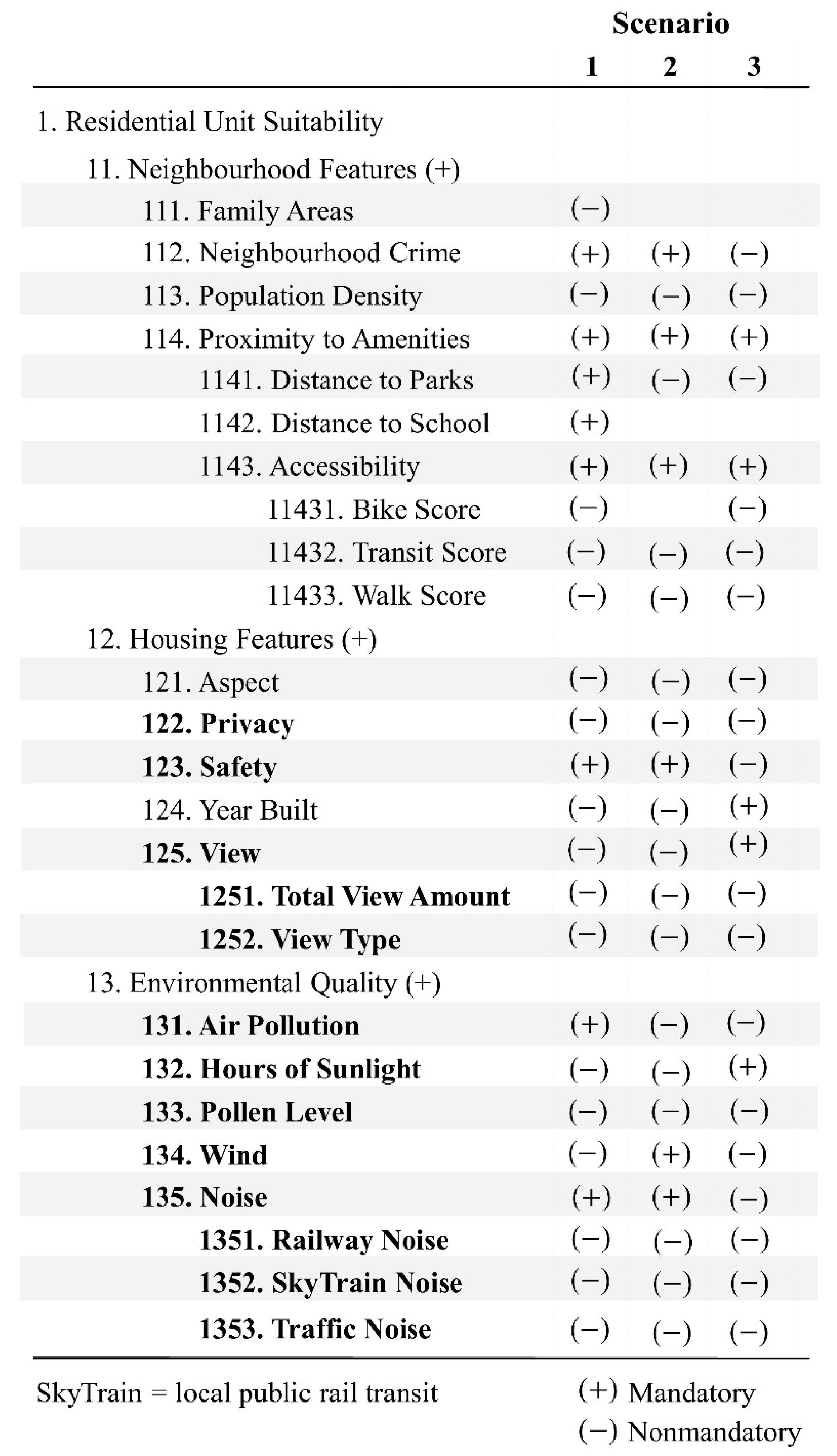
3.2. Decision Problem, LSP Attribute Tree, and Elementary Criteria

In this research, the decision problem consists of identifying the most suitable high-rise residential units for prospective residents. LSP attributes and 3D preference scenarios can be developed for various groups and stakeholders, including real-estate tax assessments, urban planners, and developers. For this study, three generalized sociodemographic groups were chosen with characteristics based on existing scientific literature: families with children (Scenario 1), elderly (Scenario 2), and working professionals (Scenario 3). Many 3D attributes, defined here as attributes whose values are affected by the vertical location of the unit, were included as factors that need to be considered in high-rise home selection in addition to the typical 2D factors and amenities. Ultimately, 10 2D and 11 3D elementary attributes influencing residence selection were identified and included in Scenario 1, three of which were omitted from either Scenario 2 or 3. The attribute trees presented for each scenario in Figure 3 are composed of three overarching attribute groups: neighborhood features (11), housing features, and (12) and environmental quality (13). The figure also distinguishes between attributes that are mandatory and nonmandatory and those that are 2D or 3D for each scenario.
The neighborhood features group (11) is composed entirely of 2D attributes. Family areas are specific to Scenario 1 and link the suitability of a neighborhood for raising a family to the number of children available to play and interact with [42]. Similarly, distance to the nearest elementary school is important to families as shorter distances reduce children’s travel time and safety risks [43]. Prospective residents may also base their decision on neighborhood crime level, which is negatively correlated with neighborhood satisfaction and mental health [44,45], or population density, which often has positive correlations with neighborhood satisfaction and smaller but stronger social networks [46,47]. Living in close proximity to urban parks is also beneficial for mental health, promotes physical activity, and provides recreational opportunities [48]. The bike, transit, and walk scores for each residential building were included as assessments of multimodal accessibility to desirable neighborhood features based on walking, cycling, or transit travel [49].
The housing features group (12) includes the compass aspect of the unit and the year the building was built, as certain orientations are typically preferred over others [50], and newer homes are generally considered more desirable [51,52]. The remaining attributes are 3D in nature. Units with a larger viewshed are more pleasing and valued higher [53], as are views that encompass desirable features, such as parks or bodies of water [54]. Safety as referred to in this study relates to the floor a unit is on; particularly, residents on higher floors will require more travel time and may encounter more hazards in the event of an emergency evacuation [55]. Privacy is also an important factor impacting home satisfaction [56,57]. Here interunit visibility was calculated as a proxy for privacy.
The environmental quality group (13) entirely comprises 3D attributes. High levels of traffic-related air pollution or tree pollen can exacerbate respiratory conditions and asthmatic attacks [58,59]. Strong winds can cause thermal discomfort or in extreme cases may pose a level of danger [60]. Excessive noise from various sources (e.g., SkyTrain, railways, cars) can negatively affect physical and mental well-being [61], while increased exposure to sunlight improves both mental and physical well-being [62].
Most elementary attribute data were not readily available and so were computed or estimated through GIS-based analyses using methods found in the literature (see Table 1). Elementary criteria functions were defined for each attribute using breakpoints based on values found in the literature (Table 1).

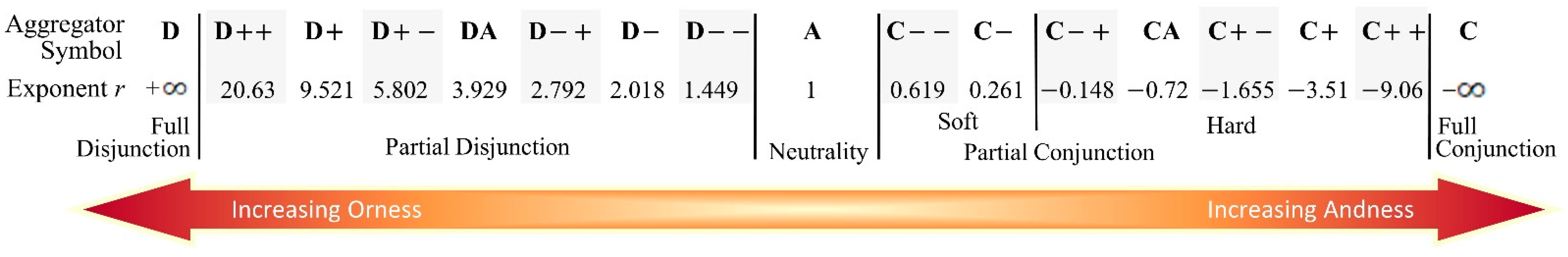
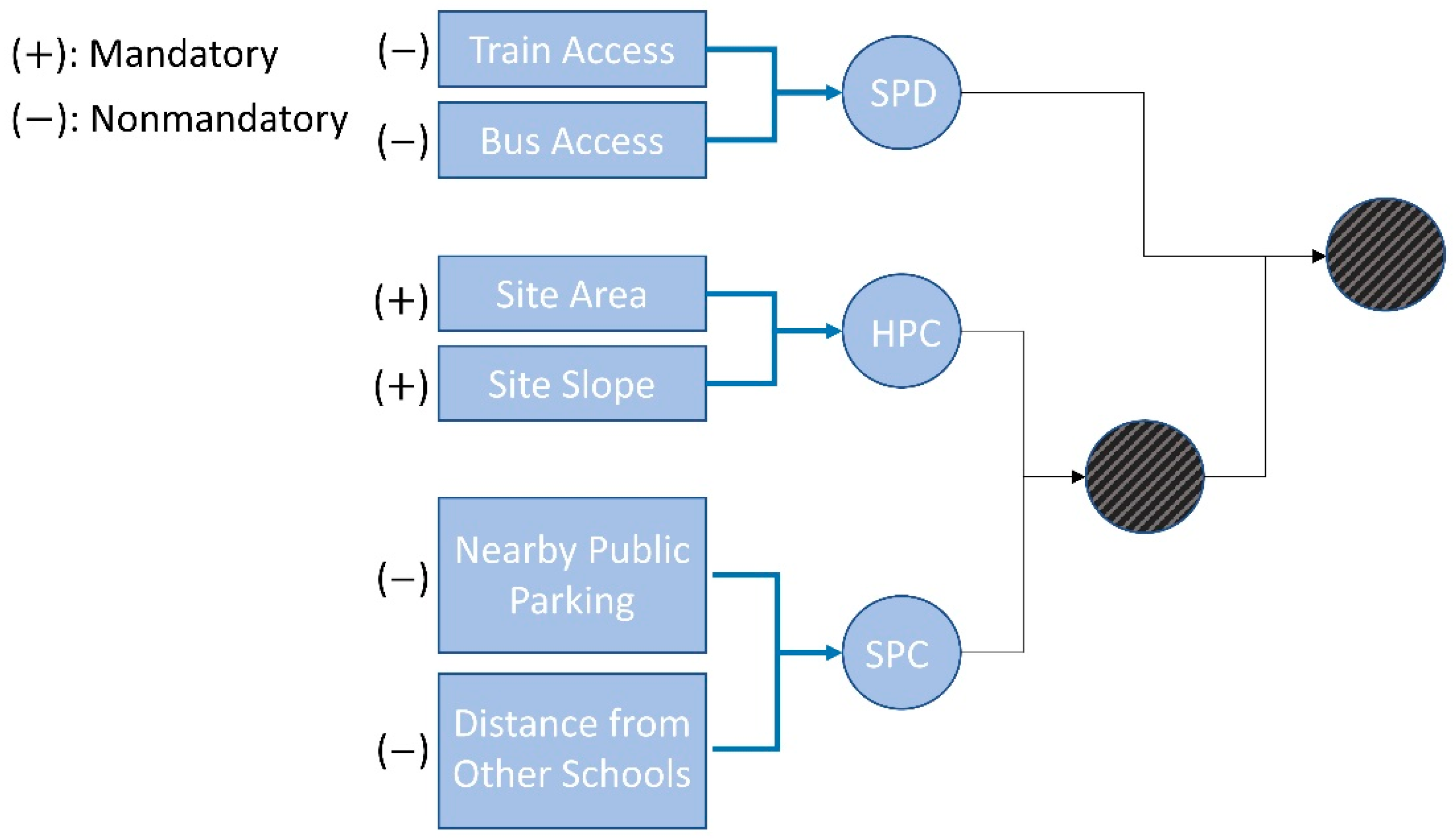
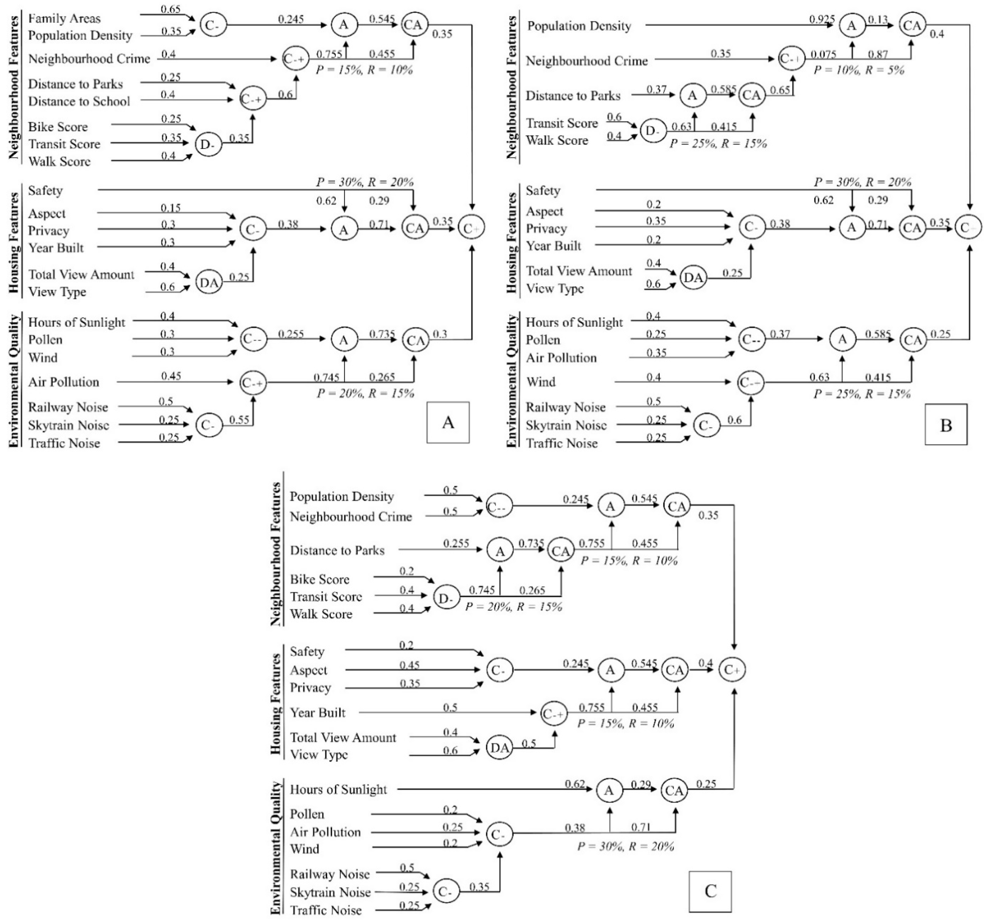
3.3. LSP Aggregation Structures

The LSP aggregation structures created for the three scenarios are depicted in Figure 4. An SPD aggregator is applied to the accessibility aggregation block (node 1143 in Figure 3) to indicate that walk, bike, and transit score criteria are replaceable to an extent, but a higher satisfaction degree is awarded to locations that satisfy all three. Similarly, an SPD aggregator is used for the view aggregation block (node 125) to suggest that while having both a large and desirable view is preferred, either criterion can partially replace the other. The remaining standard aggregators are either SPC or HPC, selected based on whether mandatory or desired components were being aggregated and the level of ANDness desired. For instance, an HPC aggregator is applied to aggregate the mandatory environment block (134–135) in Scenario 2 as they are mandatory requirements (Figure 4B), and C− + in particular is chosen to indicate that only a low to moderate level of simultaneity is needed. Both of the nonmandatory neighborhood (112–113) and nonmandatory housing (121–123) aggregation blocks in Scenario 3 are composed of desired components and thus require SPC aggregators (Figure 4C), but a larger ANDness (C−) is used for nonmandatory housing, denoting the demographic’s desire for a slightly higher level of simultaneity in having all of safety, privacy, and a desired aspect.
Criteria weights were selected based on the expected priorities for each demographic. In reality, subject matter experts or decision problem stakeholders should be consulted in determining the appropriate criteria weights, as the resulting suitability scores can be highly sensitive to input weight values. However, the weight estimations used are sufficient for the purposes of this study, as the primary goal is to demonstrate the 3D LSP–MCE approach, and the decision problem itself is subjective in nature. Some weights were identical across the three scenarios. For example, the view type is weighted as 60% of the view block (node 125) value for all prospective resident types, while the total view amount is set at 40% (Figure 4). However, most weights and, more generally, the aggregation blocks vary between scenarios. For instance, aspect is a nonmandatory attribute in all scenarios and varies in weight from 0.2 (Scenario 2) through 0.3 (Scenario 1) to a high of 0.45 for Scenario 3.
Where asymmetric logic occurs in the aggregation structures (i.e., combination of a mandatory and a desired input), a conjunctive partial absorption (CPA) aggregator must be used, in this case an A/CA aggregator combination [17]. The CPA is a compound aggregator that requires the selection of reward (R) and penalty (P) values in order to determine the relationship between the inputs and the weights assigned to them in each aggregation step [21]. R and P are percent values used, respectively, to either increase the elementary preference if the desired input is fully satisfied or decrease the preference if the desired input is not satisfied [19]. Accordingly, the magnitudes of P and R reflect the desirability of the nonmandatory input. For instance, Scenario 2 both penalizes and rewards units much higher on the combined nonmandatory housing features than it does on population density attributes, an indication of the preferences for elderly residents (Figure 4B).
To compute the 3D suitability values, elementary attribute values were converted to elementary preferences that were aggregated in a stepwise manner from the leaves of the tree structure towards the root to calculate the overall suitability score of each voxel unit in the study area buildings. Individual logic aggregators were implemented using the weighted power mean, which can be described as follows [17]:
GCD(X1, …, Xn) = [W1X1r + … + WnXnr]1/r
where GCD(X1, …, Xn) is the suitability score for an alternative with the input elementary preferences X1, …, Xn for a set of n attributes; W1, …, Wn are the weights of relative importance for the preference inputs; and r indicates the degree of simultaneity and replaceability as determined by the aggregator (Figure 1). More broadly, the overall 3D suitability score S ( v i ) for a voxel unit i located at position ( X i , Y i , Z i ) can be expressed as the output of the overarching LSP criterion function, as presented in the following extended formula:
S ( v i ) = g ( a 1 ( v i ) ,   a 2 ( v i ) ,   .   .   .   ,   a n ( v i ) )
where g is the LSP criterion function, and ( a 1 ( v i ) ,   a 2 ( v i ) ,   .   .   .   ,   a n ( v i ) ) is the array of n elementary attributes associated with the 3D voxel unit i at position ( X i , Y i , Z i ) .
A cost–suitability analysis was also conducted to compute the overall value of each unit alternative, which can be viewed as a function of the suitability and cost of a unit [16,17]. Cost is incorporated separately from suitability in this manner as it is better aligned with human reasoning [26]. The cost–suitability analysis is extended in 3D and implemented to calculate the overall value V ( v i )   for a voxel unit i located at a position ( X i , Y i , Z i ) using the following extended value indicator formula:
V ( v i ) = [ W u ( U ( v i ) ) r + W p ( P ( v i ) ) r ] 1 / r   0 W u 1 ,   0 W p 1 ,   W u + W p = 1 , r +
where U( v i ) is the usefulness indicator defining the range of acceptable suitability scores; P( v i ) is the inexpensiveness indicator defining the range of acceptable cost; W u and W p are the weights of relative importance assigned to the usefulness and inexpensiveness indicators, respectively; and r indicates the degree of simultaneity and replaceability as determined by the aggregator. Unit conveyance prices were obtained from BC Assessment [82] datasets, with missing values estimated using proximate unit prices.

4. Results and Discussion

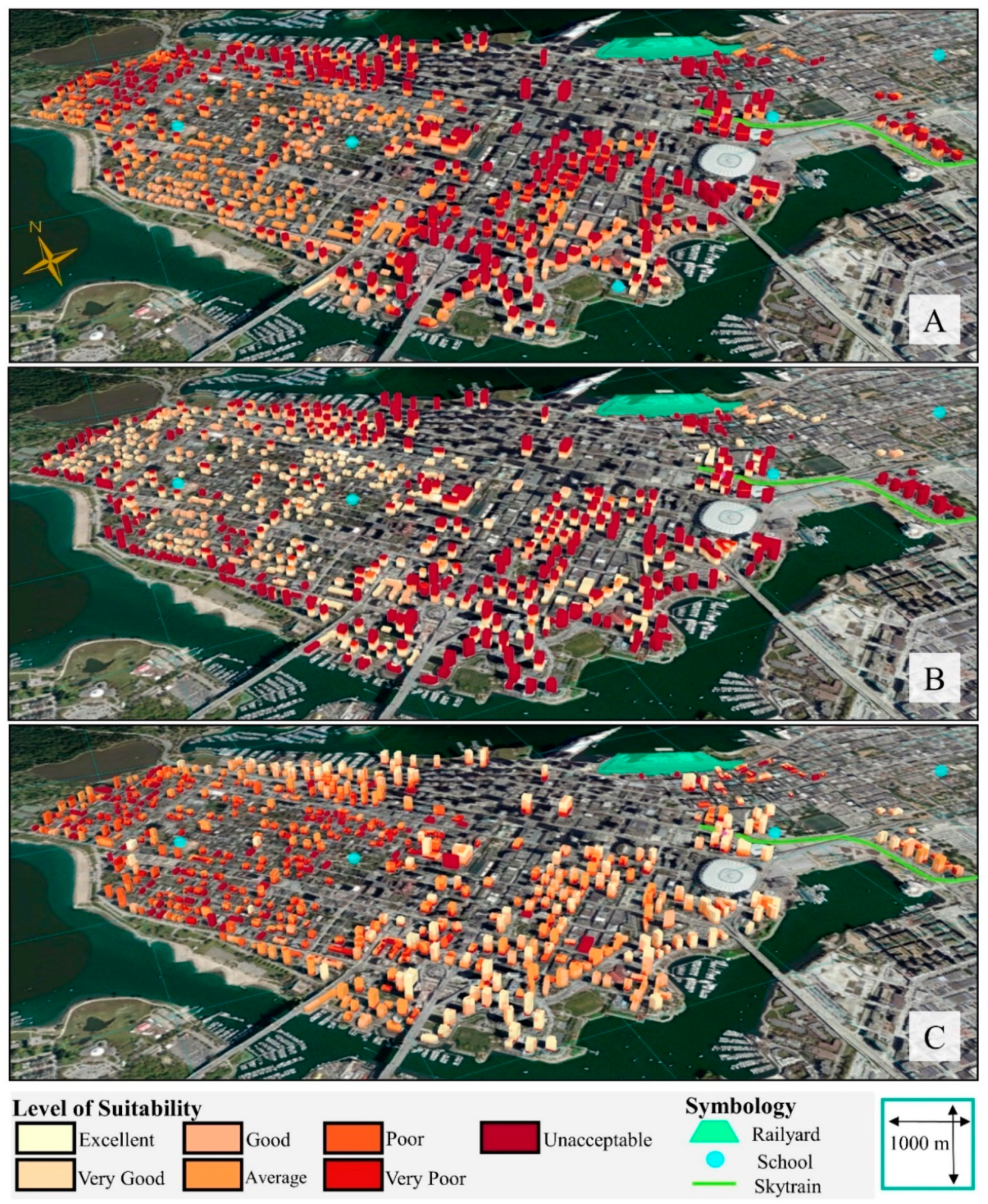
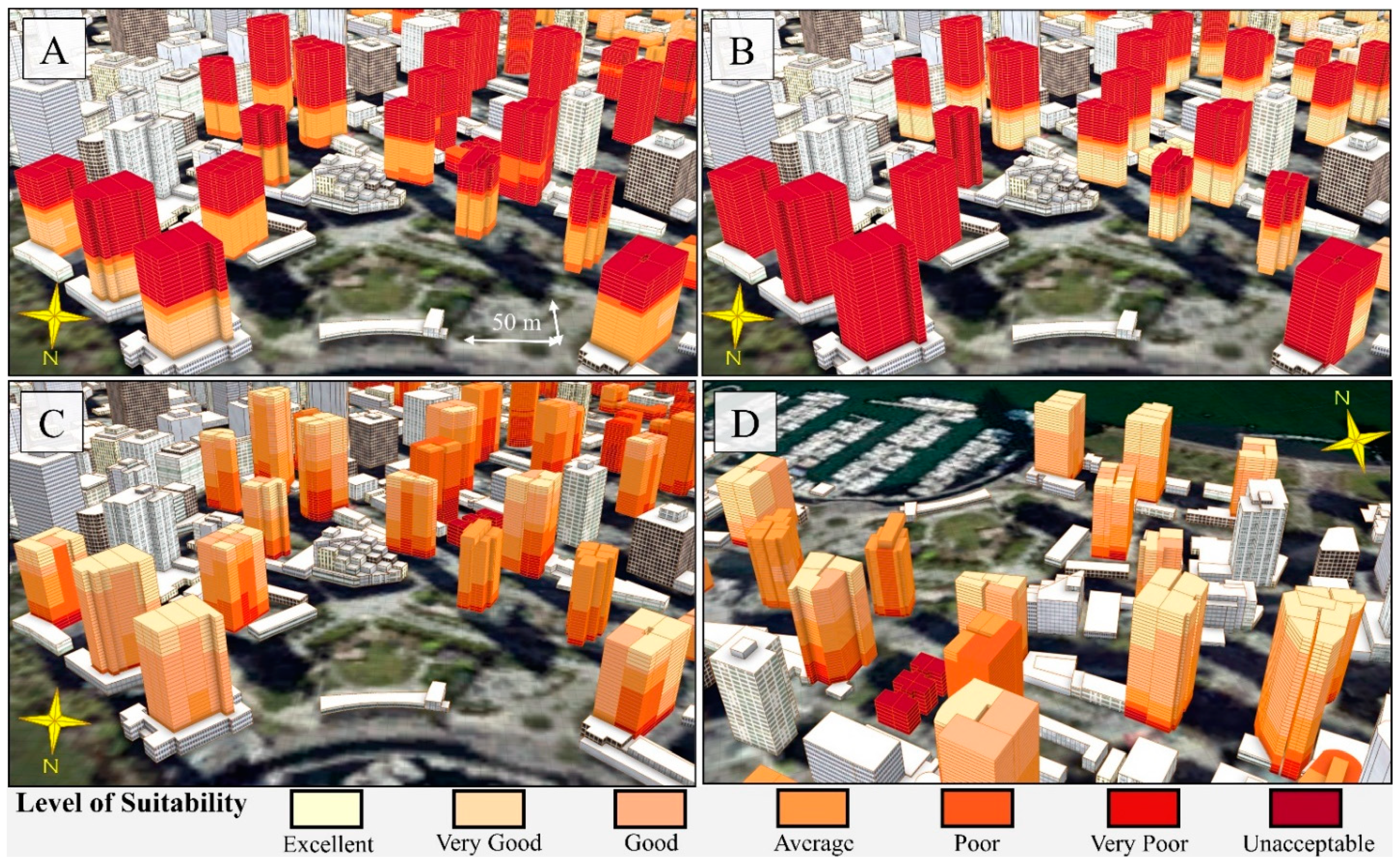
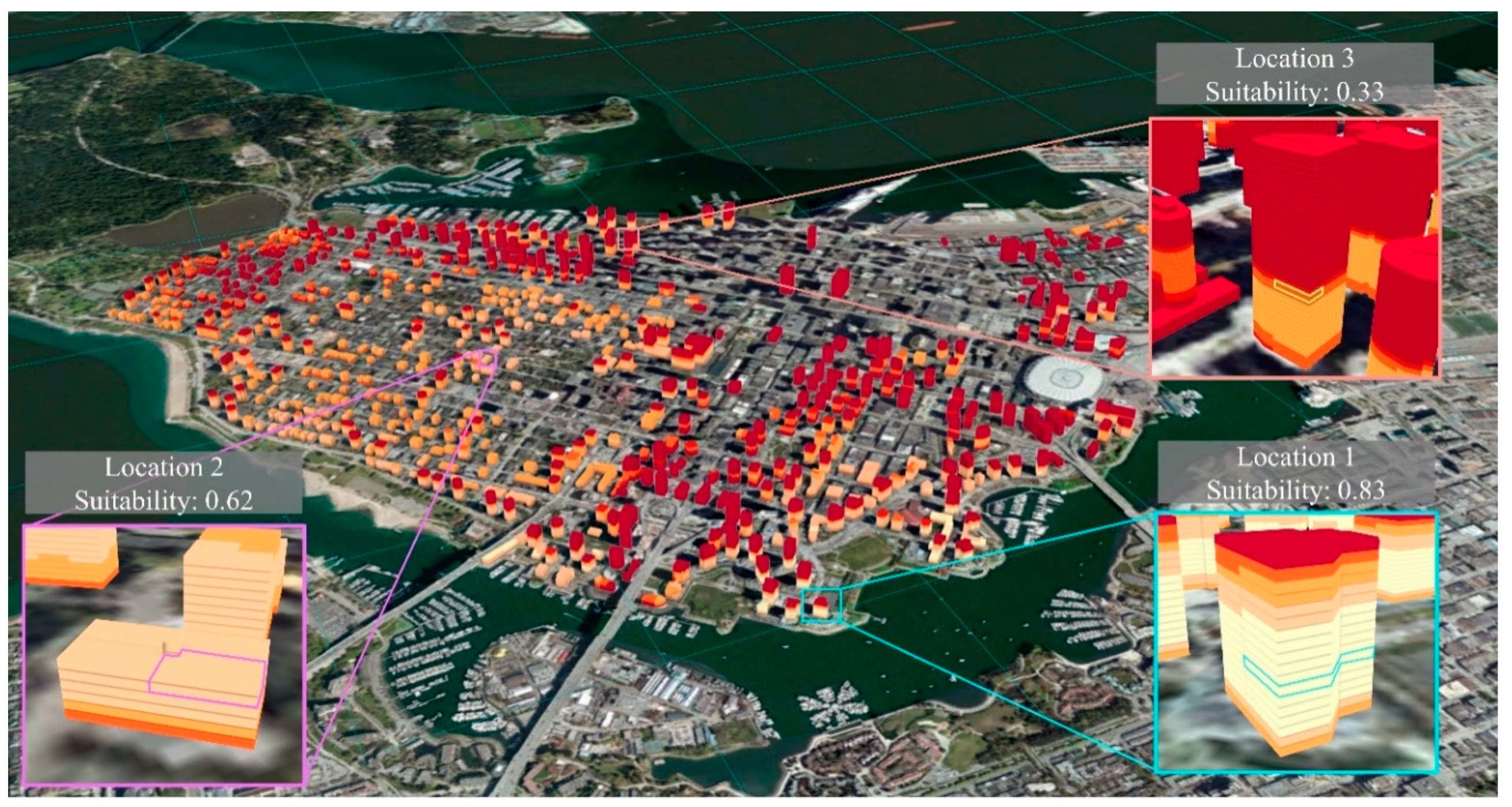
4.1. Three-Dimensional Suitability Analysis

The LSP criterion functions and 3D LSP–MCE suitability analyses were coded and run in CityEngine 2019.1 software [11] using the Computer Generated Architecture (CGA) programming language. The suitability scores for the 3D voxel units are presented and classified into seven equal interval classes of suitability: unacceptable (0.0–0.14), very poor (0.14–0.28), poor (0.28–0.43), average (0.43–0.57), good (0.57–0.71), very good (0.71–0.86), and excellent (0.88–1.00). Figure 5 presents the suitability analysis results for each scenario.
The 3D LSP–MCE suitability results vary considerably between the three scenarios. Scenario 1 is the most restrictive scenario with both the most low suitability units and the least high suitability units (Table 2). Some 44% of high-rise residential units fall within the unacceptable category, while no units are classified as excellent. Only 1% exhibit very good suitability with most confined to lower- to midlevel floors of waterfront buildings along the southern downtown boundary (Table 2, Figure 5A). This is due primarily to the scenario’s stricter requirements with a greater number of mandatory attributes. For instance, low levels of noise, crime, and air pollution are considered mandatory requirements for families, which eliminates units located in higher crime areas and near high volume streets. Safety is also mandatory, resulting in lower suitability for lower floors and lower suitability or nonsuitability for higher floors.
Although no voxel units are completely unsatisfied for the mandatory noise attribute, units near busy streets, the railyard, or the SkyTrain receive lower noise preference scores and thus lower suitability scores. Units with good or very good suitability are found primarily along the downtown periphery as they have greater access to higher weighted (≥0.4) desired attributes, such as large desirable water views and sunlight, although there is also a cluster of higher suitability voxel units towards the downtown center due to their proximity to an elementary school. The units exhibiting very good suitability along the southern downtown edge are also influenced by the high family area score of the neighborhood. Moderately suitable units in the northwest downtown region are located in areas with higher crime rates and lower percentages of families and have lower quality views and sunlight due to their central position, shorter stature, and obstructions from neighboring downtown buildings (Figure 5A).
There is considerable overlap in unacceptable units between Scenarios 1 and 2, particularly on higher floors, as both scenarios share mandatory safety, crime, and noise attributes (Figure 5A,B). However, Scenario 2 results depict many additional unacceptable units along the downtown periphery, reflecting the mandatory emphasis on a low-wind environment for the elderly demographic. Overall, Scenario 2 has the greatest number of high suitability units, with 2% and 26% of voxel units displaying excellent and very good suitability, respectively (Table 2). This may be partly attributable to having fewer mandatory attributes and partly to some high-scoring desired attributes, such as distance to parks, transit score, and walk score, being weighted relatively highly. Similar to Scenario 1, many of the highest suitability units are found along the downtown perimeter where views are generally abundant and pollution is less, but a few streets in where the wind is not as strong.
The pattern of suitability is drastically different in Scenario 3 as safety, crime, and noise are not mandatory attributes, and instead, building age, view, and sunlight are prioritized (Figure 5C). As a result, buildings located along high-volume streets or in higher crime areas are not as heavily penalized, and units on higher floors are actually preferred as they are less prone to view and sunlight obstruction. Conversely, most units on lower floors are less suitable due to restricted views and sunlight, except for buildings along the downtown periphery. Unsurprisingly, many of the high suitability units occur in waterfront buildings, which have the extra advantage of having a desirable view type. The influence of building age is also evident, with older buildings predominantly situated in the northwest region of downtown, where the majority of low suitability voxel units are located. Scenario 3 has both the most excellent suitability units and the least unacceptable units (Table 2).
Certain trends are visible across all scenarios. Figure 6 presents a subsection of the study area permitting higher detail. For instance, corner units and units on higher floors tend to exhibit higher levels of suitability as they typically have access to larger views and longer hours of sunlight. Higher levels of near-ground noise, pollen, and air pollutants further contribute to the disparity in suitability between units on higher and lower floors. Privacy also has an influence as units within viewing distance of other units or from street spectators are considered less suitable. Units near parks or water also tend to score higher as they have more desirable views than units with views of surrounding city buildings. South-oriented units (Figure 6C) typically display higher levels of suitability than those oriented north (Figure 6D) as a south aspect is generally preferred and receives more sunlight.

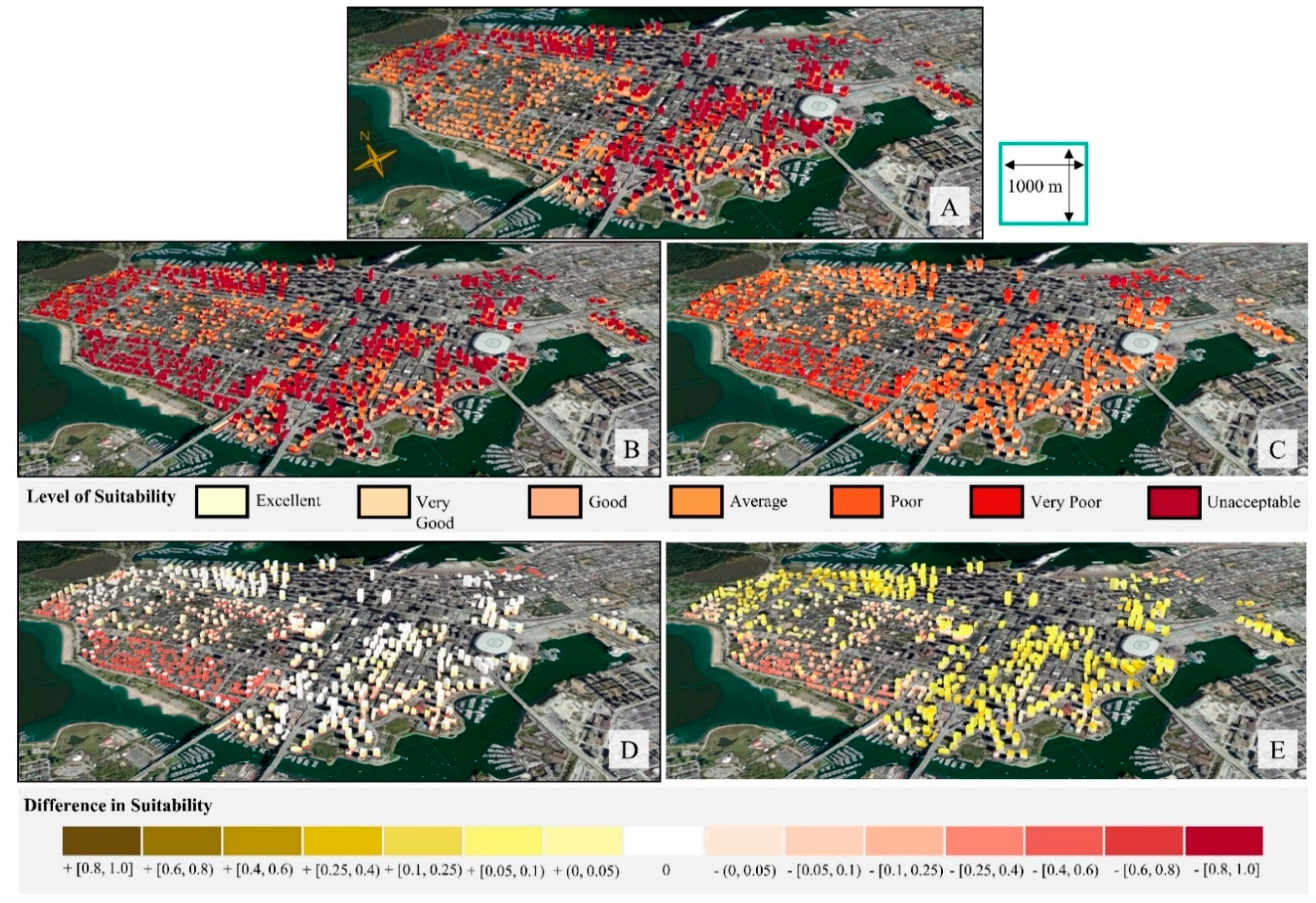
4.2. Sensitivity and Cost–Suitability Analysis

In addition to performing the 3D LSP–MCE suitability analysis, the sensitivity of parameters was tested by modifying parameters for Scenario 1 using four separate test scenarios and by comparing the obtained results. The first sensitivity test involved increasing the number of mandatory attributes for Scenario 1, namely, family areas, population density, privacy, and pollen. The second test removed all mandatory attributes from Scenario 1 such that all attributes were desired. The third test weighted all components within each aggregation block in Scenario 1 equally. Finally, the last test implemented a one-at-a-time approach by incrementally increasing the input elementary attribute and elementary preference values for three elementary criteria (traffic noise, family areas, distance to schools) and the ANDness of aggregators for three aggregation subgroups (mandatory environmental, desired environmental, mandatory neighborhood) at three residential unit locations (Figure 7) to derive sensitivity curves and influence ranges.
To visualize the change in results for the first two tests, 3D difference maps were created by subtracting the original Scenario 1 suitability value for each unit from the corresponding new suitability value. Figure 8 presents the results of the sensitivity analysis with the initial Scenario 1 provided in panel (A) as a reference. Contrasting suitability values for more and no mandatory attributes are found in panels (B) and (C), and the respective difference maps are shown in panels (D) and (E). The results of the third sensitivity analysis test with equal weights provide a very small change in obtained values for 3D suitability ranging from −0.12 to +0.05, which can be explained by the aggregation block components in Scenario 1 not having extreme differences for weights.
The addition of further mandatory attributes generates more unacceptable units compared with the original Scenario 1. This is particularly evident along the west downtown border, where the percentage of family units is relatively low (Figure 8B), although some units’ suitability has increased marginally. Overall, the range in suitability increase was minimal with a maximum increase of 0.11, compared with a maximum decrease in suitability of 0.75. The results of the second test with all nonmandatory attributes show a considerably different pattern of many fewer unacceptable units with the majority of units increasing in suitability with some exceptions, most notably in the same section as the first test results (Figure 8C). This can be explained that nonmandatory attributes that score relatively low in this area, such as family neighborhood composition and year built, now have a relatively larger influence on suitability outcome as there are no mandatory attributes. While approximately a quarter of all units have decreased in suitability by as much as −0.5, the overwhelming majority have increased by a maximum of 0.72. These results demonstrate how significantly suitability can change depending on the designation of mandatory or nonmandatory attributes, as mandatory attributes are inherently restrictive. For this reason, the LSP–MCE method should be used with direct consultation with interested groups who can provide direct input in the choice of parameters for decision-making.
Sensitivity curves from the fourth sensitivity test are presented in Figure 9 along with corresponding influence ranges for each of the three locations. Distance to school has the largest influence range of the three criteria, which can be explained by its designation as a mandatory criterion, whereas the desired criterion family areas has the smallest influence range (Figure 9A). Traffic noise is also a desired criterion, but it serves as an input for a mandatory component, which may explain its intermediate range of influence. The shapes of the curves are also significant with all following increasing concave functions with a progressively slower rate of increase in suitability for higher preference scores, although it is most pronounced for distance to school (Figure 9B). This makes sense as mandatory criteria model hard simultaneity, and therefore, suitability is more strongly limited by other potentially lower-scoring criteria in the same aggregation block. The distance to school curve starts at the origin (0,0) representing its mandatory nature and the automatic rejection of locations that do not satisfy the criterion. Another observation is that Location 1 with the highest overall suitability score also produces the greatest ranges in output suitability, while Location 3 with the lowest suitability produces the smallest ranges.
When the ANDness of aggregators is increased, the overall pattern is one of decreasing suitability as the progression towards simultaneity is more restrictive with fewer opportunities to satisfy user requirements based on other aggregation subgroup component preference scores (Figure 9C). In this case, Location 1 has the largest range in output suitability values under the desired environment subgroup, although Location 2 has the largest range under the two mandatory subgroups. Mandatory environment demonstrates the largest influence ranges of the three subgroups, which may be explained by the smaller number of input components that can ultimately impact the output preference score. The results suggest that extra care should be taken in assigning proper attribute values and calculating preference scores for the most sensitive parameters, namely, mandatory criteria, particularly where elementary preferences are low.
The cost–suitability analysis on the three scenarios was performed using unique usefulness U(vi) and inexpensiveness P(vi) indicators and associated importance weights for each scenario to represent the relative importance and range of acceptable cost for each demographic type. The calculated values of the 3D voxel units for each scenario are displayed in Figure 10 and summarized by class distribution in Table 3. The minimum suitability threshold of the usefulness indicator further restricts the overall value scores compared with the suitability scores and results in an increase in the number of unacceptable units across all scenarios (Figure 10, Table 3). Conversely, the number of higher-value units has decreased for Scenarios 2 and 3, but has actually increased significantly for Scenario 1. This can be explained by the scenario’s relatively wide range in acceptable cost values for the family demographic’s inexpensiveness indicator, which results in relatively high cost scores at voxel unit alternatives that already possessed at least a moderate degree of suitability.
In contrast, the number of higher-value voxel units in Scenario 2 has decreased as a lower acceptable price range is assigned to the elderly demographic, which reduces the desirability of higher-priced units. Working professionals are assigned a wider acceptable cost range, but higher-priced units, which typically coincide with highly suitable units in Scenario 3, receive lower inexpensiveness scores. Clearly, incorporating a cost requirement is necessary as both an important factor in residential selection decision problems and a strong influence on the overall unit value abundance and distribution. This analysis can also be interpreted as an indicator of affordability as conveyance price is a proxy for market value and the ability for the three demographic groups to afford a particular unit.

5. Conclusions

This research builds on the work of [14] by implementing a more advanced LSP–MCE method and extending it to operate in a 3D GIS environment. The suitability scenarios used in this study demonstrate the proposed method’s ability to effectively analyze the suitability of thousands of 3D unit decision alternatives based on the distinct priorities, requirements, and desires of different prospective resident demographic types. In addition, the sensitivity analysis illustrated the 3D LSP–MCE method’s responsiveness to different LSP structures as the results varied greatly across the three scenarios in terms of both the abundance and distribution of units for each suitability class. More broadly, the study provides evidence of the LSP method’s ability to accommodate various decision scenarios and flexibility in decision logic for modeling human reasoning across a large number of criteria. Furthermore, the cost–suitability analysis results support the need for incorporating the cost factor into such decision problems, as it is integral to real-world residence selection and can substantially alter alternative value outcomes.
Validation measures were not performed as the residential unit data layers were synthetically created due to privacy and data availability issues, and the LSP criterion function parameters by nature of the decision problem are highly subjective. Thus, the results are not meant necessarily to inform home-buying decisions in downtown Vancouver, but rather to demonstrate the functionality and application of the proposed 3D LSP–MCE method for a dense built environment. However, if residential data, such as precise unit floor plans, were available, the results would be improved through more accurate statistics of units under each suitability class, as well as other potential metrics, such as total floor area or volume. This study can be improved with more detailed residence data, such as information on the number of bedrooms and bathrooms and market pricing. It could also further benefit from more quantitative sensitivity analyses on other parameters, such as surveying prospective residents to refine criteria weights and designation of mandatory/desired attributes, and more accurate attribute analysis methods. For instance, inclusion of 3D vegetation data could change view attribute values considerably where lower units’ views are obscured by street trees or privacy shrubbery. Transportation infrastructure could also affect view attributes; however, this is not critical in the current study, where only one SkyTrain platform and rail exists aboveground on the periphery of the study area.
The 3D LSP–MCE method could benefit fields of study that require analysis and modeling of decision alternatives occurring across three dimensions, particularly where large numbers of attributes are involved. The wide range of decision logic aggregators allows for more expressive suitability values in 3D through criterion function structures that better reflect human reasoning in comparison with more traditional MCE methods, such as WLC, that implement a limited decision logic on a smaller number of criteria and produce less variability in output 3D scores. The study could be extended by including more relevant criteria, analyzing a larger study area of a built environment, or by considering different user group requirements. In addition, it could be applied to much denser built environments, such as those in Asian, US, or larger European cities, to examine and compare the effects of different potential evaluation criteria and their aggregations. The proposed method can assist urban planners and developers in assessing various urban development scenarios by analyzing the impacts of new development on neighboring buildings. More broadly, the 3D LSP–MCE approach developed in this research study can support spatial decision-making in real time or in applications that require analysis and representation in 3D, such as management of the housing market, urban property, and tax assessments.

Author Contributions

Conceptualization, K.M., S.D. and R.F.; methodology, K.M., S.D. and R.F.; software, S.D. and K.M.; validation, K.M.; formal analysis, K.M., S.D. and R.F.; investigation, K.M., S.D. and R.F.; resources, S.D.; data curation, K.M.; writing—original draft preparation, K.M.; writing—review and editing, S.D., R.F. and K.M.; visualization, K.M.; supervision, S.D. and R.F.; project administration, S.D.; funding acquisition, S.D. All authors have read and agreed to the published version of the manuscript.

Funding

This research was funded by the Natural Sciences and Engineering Research Council of Canada (NSERC) grant number RGPIN-2017-03939 and the Canada Graduate Scholarships Master’s Program (CGSM). The article processing charges (APC) were fully funded by the Simon Fraser University Central Open Access Fund.

Data Availability Statement

This research uses some data derived directly from sources that prohibit redistribution or publication, and so they would not be available for sharing.

Acknowledgments

The authors would like to thank BC Assessment for providing data on residential units in Metro Vancouver. They would also like to thank Simon Fraser University’s GIS and Map Librarian Sarah Zhang for her guidance in locating geospatial data. In addition, we are thankful to the four anonymous reviewers for their valuable feedback.

Conflicts of Interest

The authors declare no conflict of interest.

References

  1. Shen, L.; Zhou, J.; Skitmore, M.; Xia, B. Application of a hybrid Entropy–McKinsey Matrix method in evaluating sustainable urbanization: A China case study. Cities 2015, 42, 186–194. [Google Scholar] [CrossRef] [Green Version]
  2. Kaur, M.; Hewage, K.; Sadiq, R. Investigating the impacts of urban densification on buried water infrastructure through DPSIR framework. J. Clean. Prod. 2020, 259, 120897. [Google Scholar] [CrossRef]
  3. Amer, M.; Mustafa, A.; Teller, J.; Attia, S.; Reiter, S. A methodology to determine the potential of urban densification through roof stacking. Sustain. Cities Soc. 2017, 35, 677–691. [Google Scholar] [CrossRef]
  4. Boyko, C.T.; Cooper, R. Clarifying and re-conceptualizing density. Prog. Plan. 2011, 76, 1–61. [Google Scholar] [CrossRef]
  5. Koziatek, O.; Dragićević, S. A local and regional spatial index for measuring three-dimensional urban compactness growth. Environ. Plan. B Urban Anal. City Sci. 2019, 46, 143–164. [Google Scholar] [CrossRef]
  6. Ying, Y.; Koeva, M.; Kuffer, M.; Asiama, K.O.; Li, X.; Zevenbergen, J. Making the Third Dimension (3D) Explicit in Hedonic Price Modelling: A Case Study of Xi’an, China. Land 2021, 10, 24. [Google Scholar] [CrossRef]
  7. Malczewski, J.; Jankowski, P. Emerging trends and research frontiers in spatial multicriteria analysis. Int. J. Geogr. Inf. Sci. 2020, 34, 1257–1282. [Google Scholar] [CrossRef]
  8. Malczewski, J.; Rinner, C. Multicriteria Decision Analysis in Geographic Information Science; Springer: Berlin/Heidelberg, Germany, 2015. [Google Scholar] [CrossRef]
  9. Autodesk. Revit; Version 2022; Autodesk: San Rafael, CA, USA, 2022; Available online: https://www.autodesk.ca/en/products/revit/overview?term=1-YEAR&tab=subscription (accessed on 10 December 2021).
  10. ESRI. ArcGIS Urban. 2022. [Online Software]. Available online: https://www.esri.com/en-us/arcgis/products/arcgis-urban/overview (accessed on 10 December 2021).
  11. ESRI. CityEngine, Version 2019.1; ESRI: Redlands, CA, USA, 2019. Available online: https://www.esri.com/en-us/arcgis/products/esri-cityengine/overview (accessed on 10 December 2021).
  12. Trubka, R.; Glackin, S.; Lade, O.; Pettit, C. A web-based 3D visualisation and assessment system for urban precinct scenario modelling. ISPRS J. Photogramm. Remote Sens. 2016, 117, 175–186. [Google Scholar] [CrossRef]
  13. Saran, S.; Oberai, K.; Wate, P.; Konde, A.; Dutta, A.; Kumar, K.; Kumar, A.S. Utilities of virtual 3D city models based on CityGML: Various use cases. J. Indian Soc. Remote Sens. 2018, 46, 957–972. [Google Scholar] [CrossRef]
  14. Munn, K.; Dragićević, S. Spatial multi-criteria evaluation in 3D context: Suitability analysis of urban vertical development. Cartogr. Geogr. Inf. Sci. 2021, 48, 105–123. [Google Scholar] [CrossRef]
  15. Montgomery, B.; Dragićević, S. Comparison of GIS-based logic scoring of preference and multicriteria evaluation methods: Urban land use suitability. Geogr. Anal. 2016, 48, 427–447. [Google Scholar] [CrossRef]
  16. Dujmović, J.; de Tré, G.; Dragićević, S. Comparison of multicriteria methods for land-use suitability assessment. In Proceedings of the 2009 IFSA World Congress/EUSFLAT Conference, Lisbon, Portugal, 20–24 July 2009; pp. 1404–1409. [Google Scholar]
  17. Dujmović, J. Soft Computing Evaluation Logic: The LSP Decision Method and Its Applications; John Wiley & Sons: Hoboken, NJ, USA, 2018. [Google Scholar]
  18. Dragićević, S.; Dujmović, J.; Minardi, R. Modeling urban land-use suitability with soft computing: The GIS-LSP method. In GeoComputational Analysis and Modeling of Regional Systems; Thill, J.-C., Dragicevic, S., Eds.; Springer International Publishing: Cham, Switzerland, 2018; pp. 257–275. [Google Scholar] [CrossRef]
  19. Dujmović, J.; Scheer, D. Logic aggregation of suitability maps. In Proceedings of the 2010 IEEE World Congress on Computational Intelligence, WCCI 2010, Barcelona, Spain, 18–23 July 2010; Volume 1, pp. 1–8. [Google Scholar] [CrossRef]
  20. Rebolledo, B.; Gil, A.; Flotats, X.; Sánchez, J.Á. Assessment of groundwater vulnerability to nitrates from agricultural sources using a GIS-compatible logic multicriteria model. J. Environ. Manag. 2016, 171, 70–80. [Google Scholar] [CrossRef] [Green Version]
  21. Dujmović, J.; de Tré, G.; van de Weghe, N. LSP suitability maps. Soft Comput. 2010, 14, 421–434. [Google Scholar] [CrossRef]
  22. Dujmović, J.; Allen, W.L. Soft computing logic decision making in strategic conservation planning for water quality protection. Ecol. Inform. 2021, 61, 101167. [Google Scholar] [CrossRef]
  23. Pirmanto, D.; Suseno, J.E.; Adi, K. Logic Scoring of Preference Method for Determining Landfill with Geographic Information System. In Proceedings of the 2018 International Seminar on Research of Information Technology and Intelligent Systems (ISRITI), Yogyakarta, Indonesia, 21–22 November 2018; pp. 459–464. [Google Scholar] [CrossRef]
  24. Luan, C.; Liu, R.; Peng, S. Land-use suitability assessment for urban development using a GIS-based soft computing approach: A case study of Ili Valley, China. Ecol. Indic. 2021, 123, 107333. [Google Scholar] [CrossRef]
  25. Shen, S.; Dragicevic, S.; Dujmović, J. GIS.LSP: A soft computing logic method and tool for geospatial suitability analysis. Trans. GIS 2021, 89, 101654. [Google Scholar] [CrossRef]
  26. Dujmović, J.; de Tré, G. Multicriteria methods and logic aggregation in suitability maps. Int. J. Intell. Syst. 2011, 26, 971–1001. [Google Scholar] [CrossRef]
  27. Statistics Canada. Census Data. 2020. Available online: https://www12.statcan.gc.ca/datasets/index-eng.cfm?Temporal=2016 (accessed on 20 July 2021).
  28. Metro Vancouver. Metro Vancouver 2040 Shaping Our Future; Metro Vancouver: Vancouver, BC, Canada, 2015. [Google Scholar]
  29. Statistics Canada. Classification by Type of Building. 2021. Available online: https://www23.statcan.gc.ca/imdb/p3VD.pl?Function=getVD&TVD=1226827&CVD=1226832&CPV=1.1&CST=01012019&CLV=2&MLV=3 (accessed on 10 December 2020).
  30. Macdonald, E. Chapter 5—Urban design for sustainable and livable communities: The case of Vancouver. In Transportation, Land Use, and Environmental Planning; Elsevier: Amsterdam, The Netherlands, 2020; pp. 83–104. [Google Scholar] [CrossRef]
  31. City of Vancouver. Open Data Portal. 2021. Available online: https://opendata.vancouver.ca/pages/home/ (accessed on 6 December 2020).
  32. BC Assessment. Assessment Search Tool. 2021. Available online: https://www.bcassessment.ca/ (accessed on 6 December 2020).
  33. City of Vancouver. VanMap: View, Search, Create, and Print Maps of Vancouver. 2017. Available online: http://vancouver.ca/your-government/vanmap.aspx (accessed on 7 November 2020).
  34. DMTI Spatial Inc. Abacus Dataverse Network: Geospatial Data Sets. CanMap RouteLogistics, v.2014.3. 2014. Available online: https://www.lib.sfu.ca/find/other-materials/data-gis/gis/spatial-data (accessed on 1 July 2020).
  35. DMTI Spatial Inc. Abacus Dataverse Network: Geospatial Data Sets. CanMap Content Suite, v2019.3. 2019. Available online: https://www.lib.sfu.ca/find/other-materials/data-gis/gis/spatial-data (accessed on 1 July 2020).
  36. University of Toronto. CHASS Canadian Census Analyser. 2017. Available online: http://dc1.chass.utoronto.ca/census/index.html (accessed on 11 July 2017).
  37. Vancouver Police Department. Vancouver Police Department Crime Data Download. 2021. Available online: https://geodash.vpd.ca/opendata/ (accessed on 7 November 2020).
  38. Government of Canada. High Resolution Digital Elevation Model (HRDEM)—CanElevation Series. 2020. Available online: https://open.canada.ca/data/en/dataset/957782bf-847c-4644-a757-e383c0057995 (accessed on 1 July 2020).
  39. Metro Vancouver. Metro Vancouver Open Data Catalogue 2016. Generalized Land Use Classification. 2020. Available online: http://www.metrovancouver.org/data (accessed on 7 November 2020).
  40. Government of British Columbia. DataBC. 2021. Available online: https://data.gov.bc.ca/ (accessed on 12 December 2020).
  41. ESRI. ArcGIS, version 10.7.1; ESRI: Redlands, CA, USA, 2019. [Google Scholar]
  42. Mee, K.J. ‘Any place to raise children is a good place’: Children, housing and neighbourhoods in inner Newcastle, Australia. Child. Geogr. 2010, 8, 193–211. [Google Scholar] [CrossRef]
  43. Martin, S.; Carlson, S. Barriers to children walking to or from school—United States, 2004. J. Am. Med. Assoc. 2005, 294, 2160–2162. [Google Scholar] [CrossRef] [Green Version]
  44. Mccrea, R.; Stimson, R.; Western, J. Testing a moderated model of satisfaction with urban living using data for Brisbane-South East Queensland, Australia. Soc. Indic. Res. 2005, 72, 121–152. [Google Scholar] [CrossRef] [Green Version]
  45. Leslie, E.; Cerin, E. Are perceptions of the local environment related to neighbourhood satisfaction and mental health in adults? Prev. Med. 2008, 47, 273–278. [Google Scholar] [CrossRef] [PubMed]
  46. Mouratidis, K. Is compact city livable? The impact of compact versus sprawled neighbourhoods on neighbourhood satisfaction. Urban Stud. 2018, 55, 2408–2430. [Google Scholar] [CrossRef]
  47. Raman, S. Designing a liveable compact city: Physical forms of city and social life in urban neighbourhoods. Built Environ. 2010, 36, 63–80. [Google Scholar] [CrossRef]
  48. Wood, L.; Hooper, P.; Foster, S.; Bull, F. Public green spaces and positive mental health—Investigating the relationship between access, quantity and types of parks and mental wellbeing. Health Place 2017, 48, 63–71. [Google Scholar] [CrossRef] [PubMed]
  49. Walk Score. Walk Score: Live Where You Love. 2021. Available online: https://www.walkscore.com/ (accessed on 1 February 2021).
  50. Huang, Z.; Chen, R.; Xu, D.; Zhou, W. Spatial and hedonic analysis of housing prices in Shanghai. Habitat Int. 2017, 67, 69–78. [Google Scholar] [CrossRef]
  51. Zortuk, M. An evaluation of higher education students’ apartment preferences: A real world study in a newly urbanized city. Istanb. Univ. Econom. Stat. e-J. 2014, 0, 1–20. [Google Scholar]
  52. Bina, M.; Warburg, V.; Kockelman, K.M. Location choice vis-à-vis transportation: Apartment dwellers. Transp. Res. Rec. 2006, 1977, 93–102. [Google Scholar] [CrossRef]
  53. Samarasinghe, O.E.; Sharp, B.M.H. The value of a view: A spatial hedonic analysis. N. Z. Econ. Pap. 2008, 42, 59–78. [Google Scholar] [CrossRef]
  54. Yasumoto, S.; Jones, A.P.; Nakaya, T.; Yano, K. The use of a virtual city model for assessing equity in access to views. Comput. Environ. Urban Syst. 2011, 35, 464–473. [Google Scholar] [CrossRef]
  55. Craighead, G. High-Rise Security and Fire Life Safety; Butterworth-Heinemann: Oksford, UK, 2009. [Google Scholar]
  56. Ghani, S.A. A changing pattern of house market in Kuala Lumpur. In Proceedings of the National Conference on Affordable Quality Housing, Miri, Sarawak, Malaysia, 24–26 November 2004; pp. 24–26. [Google Scholar]
  57. Hashim, A.H.; Ali, H.M.; Samah, A.A. Urban Malay’s user-behaviour and perspective on privacy and spatial organization of housing. ArchNet-IJAR 2009, 3, 197–208. [Google Scholar]
  58. Xie, X.; Semanjski, I.; Gautama, S.; Tsiligianni, E.; Deligiannis, N.; Rajan, R.T.; Pasveer, F.; Philips, W. A review of urban air pollution monitoring and exposure assessment methods. ISPRS Int. J. Geo-Inf. 2017, 6, 389. [Google Scholar] [CrossRef] [Green Version]
  59. Kasprzyk, I.; Ćwik, A.; Kluska, K.; Wójcik, T.; Cariñanos, P. Allergenic pollen concentrations in the air of urban parks in relation to their vegetation. Urban For. Urban Green. 2019, 46, 126486. [Google Scholar] [CrossRef]
  60. Reiter, S. Assessing wind comfort in urban planning. Environ. Plan. B Plan. Des. 2010, 37, 857–873. [Google Scholar] [CrossRef] [Green Version]
  61. Kim, A.; Sung, J.H.; Bang, J.-H.; Cho, S.W.; Lee, J.; Sim, C.S. Effects of self-reported sensitivity and road-traffic noise levels on the immune system. PLoS ONE 2017, 12, e0187084. [Google Scholar] [CrossRef] [PubMed]
  62. Swanson, V.; Sharpe, T.; Porteous, C.; Hunter, C.; Shearer, D. Indoor annual sunlight opportunity in domestic dwellings may predict well-being in urban residents in scotland. Ecopsychology 2016, 8, 121–130. [Google Scholar] [CrossRef] [Green Version]
  63. City of Vancouver. Greenest City—2020 Action Plan; City of Vancouver: Vancouver, BC, Canada, 2012; p. 82. [Google Scholar]
  64. Vancouver Board of Parks and Recreation. Vancouver Park Provision Study; Vancouver Board of Parks and Recreation: Vancouver, BC, Canada, 2018.
  65. Vancouver Board of Education. Long Range Facilities Plan; Vancouver Board of Education: Vancouver, BC, Canada, 2015.
  66. Lu, J. The value of a south-facing orientation: A hedonic pricing analysis of the Shanghai housing market. Habitat Int. 2018, 81, 24–32. [Google Scholar] [CrossRef]
  67. Shach-Pinsly, D. Visual openness and visual exposure analysis models used as evaluation tools during the urban design development process. J. Urban. 2010, 3, 161–184. [Google Scholar] [CrossRef]
  68. Robinson, M.B.; Robinson, C.E. Environmental characteristics associated with residential burglaries of student apartment complexes. Environ. Behav. 1997, 29, 657–675. [Google Scholar] [CrossRef] [Green Version]
  69. Gordon, B.; Winkler, D.; Barrett, D.; Zumpano, L. The effect of elevation and corner location on oceanfront condominium value. J. Real Estate Res. 2013, 35, 345–364. [Google Scholar] [CrossRef]
  70. Proulx, G.; Mcqueen, C. Evacuation Timing in Apartment Buildings; National Research Council of Canada. Institute for Research in Construction: Ottawa, ON, Canada, 1994.
  71. The Condo Group. How to Spot a Leaky Condo. 2011. Available online: https://thecondogroup.com/how-to-spot-a-leaky-condo/ (accessed on 7 November 2020).
  72. Metro Vancouver. Metro Vancouver Housing Data Book; Metro Vancouver: Vancouver, BC, Canada, 2019. [Google Scholar]
  73. Bourassa, S.C.; Hoesli, M.; Sun, J. What’s in a view? Environ. Plan. A Econ. Space 2004, 36, 1427–1450. [Google Scholar] [CrossRef]
  74. Metro Vancouver. Caring for the Air 2020; Metro Vancouver: Vancouver, BC, Canada, 2020. [Google Scholar]
  75. Yasumoto, S.; Jones, A.; Yano, K.; Nakaya, T. Virtual city models for assessing environmental equity of access to sunlight: A case study of Kyoto, Japan. Int. J. Geogr. Inf. Sci. 2012, 26, 1–13. [Google Scholar] [CrossRef]
  76. Rojo, J.; Oteros, J.; Pérez-Badia, R.; Cervigón, P.; Ferencova, Z.; Gutiérrez-Bustillo, M.A.; Bergmann, K.-C.; Oliver, G.; Thibaudon, M.; Albertini, R.; et al. Near-ground effect of height on pollen exposure. Environ. Res. 2019, 174, 160–169. [Google Scholar] [CrossRef] [PubMed]
  77. Wong, M.S.; Nichol, J.E.; To, P.H.; Wang, J. A simple method for designation of urban ventilation corridors and its application to urban heat island analysis. Build. Environ. 2010, 45, 1880–1889. [Google Scholar] [CrossRef]
  78. Wakefield Acoustics Ltd. City of Vancouver Noise Control Manual; Wakefield Acoustics Ltd.: Victoria, BC, Canada, 2004. [Google Scholar]
  79. Health Canada. Guidance for Evaluating Human Health Impacts in Environmental Assessment: Noise; Health Canada: Ottawa, ON, Canada, 2017; Volume 53.
  80. BKL Consultants Ltd. Cargill Rail Expansion Project: Environmental Noise Assessment. North Vancouver. 2015. Available online: https://www.portvancouver.com/wp-content/uploads/2015/03/3057-15a-cargill-rail-expansion-environmental-noise-assessment_final.pdf (accessed on 7 November 2020).
  81. SLR Consulting Ltd. SkyTrain Noise Study Vancouver. Vancouver, Canada. 2018. Available online: https://www.translink.ca/-/media/translink/documents/plans-and-projects/skytrain-noise-study/skytrain-noise-report-20181128.pdf (accessed on 7 November 2020).
  82. BC Assessment. Custom Dataset; BC Assessment: Nanaimo, BC, Canada, 2021. [Google Scholar]
Figure 1. Logic scoring of preference (LSP) logic aggregators with associated symbols and r exponent values.
Land 11 00443 g001
Figure 2. Sample LSP aggregation structure for selecting a location for a new college.
Land 11 00443 g002
Figure 3. Attribute tree with elementary attributes for the three scenarios with 3D attributes highlighted in bold text.
Land 11 00443 g003
Figure 4. LSP aggregation structures for (A) Scenario 1 (family oriented), (B) Scenario 2 (elderly oriented), and (C) Scenario 3 (working professionals oriented).
Land 11 00443 g004
Figure 5. Results of the 3D LSP multicriteria evaluation (MCE) suitability analysis for Scenarios (A) 1, (B) 2, and (C) 3.
Land 11 00443 g005
Figure 6. Suitability values obtained from the 3D LSP–MCE analysis for a subset of buildings under Scenarios (A) 1, (B) 2, and (C) 3 facing south and (D) Scenario 3 facing north.
Land 11 00443 g006
Figure 7. The three residential units selected for the one-at-a-time sensitivity tests with associated suitability scores for Scenario 1.
Land 11 00443 g007
Figure 8. The 3D suitability maps for initial Scenario 1 (A) and the sensitivity analysis results for Scenario 1 with (B) more mandatory attributes and (C) no mandatory attributes and the calculated corresponding 3D difference maps (D,E), respectively. Change in overall suitability compared with the original Scenario 1 is expressed as the increase or decrease in suitability resulting from parameter variation.
Land 11 00443 g008
Figure 9. Sensitivity curves obtained for three locations using varying values for (A) input elementary attributes and (B) input elementary preferences for three elementary criteria and (C) aggregators of varying ANDness for three aggregation subgroups.
Land 11 00443 g009
Figure 10. Results of the cost–suitability analysis for (A) Scenarios 1, (B) 2, and (C) 3.
Land 11 00443 g010
Table 1. Elementary attribute criteria in vertex notation format with associated criterion function breakpoints and rationale. Attributes that are 3D in nature are highlighted in bold text.
AttributeAnalysis MethodRationale
Neighborhood FeaturesFamily Areas{(20,0), (80,1)}
(percentile of all census tract areas % occupied dwellings with children)
Preferences of 0 and 1 assigned to 20th and 80th percentile values, respectively, as more children means more peers to interact with.
Analysis: Percentage of occupied dwellings with families.
Neighborhood Crime{(0–0.005,1), (0.005–0.0015,0.8), (0.0015–0.005,0.6), (0.005–0.01,0.4), (0.01–0.02,0.2), (0.02,0)}
(crime density)
Crime is negatively correlated with neighborhood satisfaction and mental health [44], so lower crime level is preferred.
Analysis: Kernel density of geolocated crime incidents.
Population Density{(29,0), (211,1)}
(people per ha in each census tract)
Based on the density-satisfaction study of [46], which averaged 29 people/ha for low-density neighborhoods and 211 people/ha for high-density neighborhoods.
Analysis: Population density.
Distance to Parks{(400,1), (800,0)}
(m)
City of Vancouver aimed to have every resident within 5 min’ walk (400 m) of a green space [63]; 99% are within 10 min’ walk (800 m) [64].
Analysis: Network distance.
Distance to School{(400,1), (2000,0)}
(m)
Preference of 1 assigned to 5 min’ walk, 0 to 25 min’ walk (2000 m), putting the 50% mark close to the average distance of 1274 m [65].
Analysis: Network distance.
Bike Score,
Transit Score,
Walk Score
{(0–24,0), (25–49,0.25), (50–69,0.5), (70–89,0.75), (90–100,1)
(score)
Based on walk score’s [49] score class ranges and score values.
Housing FeaturesAspect{(N, 0), (NE/NW, 0.25), (E/W, 0.5), (SE/SW, 0.75), (S, 1)}
(aspect)
How property values proportionally increase with different aspects is presented in [66].
Analysis: Determine unit aspect(s) using building and unit footprints and linear directional mean tool.
Privacy{(Low, 0), (relatively low, 0.33), (medium, 0.67), (high, 1)}
(privacy level)
Four levels of visual exposure are defined in [67]: low (>50 m from nearest view point); relatively low (25–50 m), medium (10–25 m), and high (<10 m).
Analysis: Intervisibility.
Safety{(1,0.5), (2,0.75), (3,1), (7,1), (18,0)}(floor number)First few floors [68,69] are more likely to be burglarized, while typical aerial ladder reach limits fire rescue to about the seventh floor [55]. Average time to descend one floor is 16.4 s [70]; 18th floor is equivalent to 5 min’ evacuation time.
Year Built{(1960, 0), (1983, 0.42), (1984, 0.1), (1998, 0.35), (1999, 0.71), (2015, 1)}
(year built)
Newer homes are generally more desirable, but 1984–1998 buildings are from Vancouver’s “leaky condo era” and may be prone to leaks [71]. Buildings from 2015 onwards built under the most recent National Building Code. Only 8% of Metro Vancouver high-rises built before 1961 [72].
Total View Amount{(10,0), (90,1)}
(percentile of view amount (m2) results)
Larger views are more pleasing and positively correlated with property prices [53,73].
Analysis: Visibility [54].
View Type{(0,0), (100,1)}
(% desirable view)
Properties with larger views of desirable view features (e.g., water) are priced higher than properties with smaller views [53].
Analysis: Overlay of visibility output and raster of desirable/undesirable view features.
Environmental QualityAir Pollution{(7,1), (17,0)}
(ppb NO2)
Metro Vancouver’s air quality objective for NO2 is an annual average of 17 ppb. Areas of cleaner air in Metro Vancouver average around 7 ppb [74].
Hours of Sunlight{(0,0), (12,1)}
(h)
More hours of direct sunlight is considered desirable due to its beneficial effects [62].
Analysis: Points solar radiation [75] for the equinox.
Pollen Level{(2,0), (12,1)}
(m above ground level)
Although pollen level decreases with height, the most significant decrease generally occurs within 10 m, with concentrations at ground level ~1.5 times higher than those 10 m higher [76].
Wind{(low, 1), (moderate, 0.75), (very low, 0.5), (high, 0.25), (very high, 0)}
(ventilation potential)
High wind speeds can bring thermal discomfort or even a level of danger [60]. In the mild Vancouver climate, a low to moderate amount of ventilation would be more appreciated.
Analysis: Computed relative wind level for three 50 m height increments [77] using most predominant winds in Vancouver.
Railway Noise,
SkyTrain Noise,
Traffic Noise
{(45,1), (95,0)}
(dBA)
Sleep disruption can occur at a sustained noise level of ≥30 dBA. More severe consequences (e.g., hearing damage) can occur at levels of ≥80 dBA [78]. However, it is assumed that transmission loss at windows is ~15 dBA [79].
Railway analysis: Estimated using similar site noise map digitization and extrapolation [80].
SkyTrain analysis: Estimated using digitization and extrapolation of SkyTrain noise maps [81].
Traffic analysis: Estimated using traffic noise equation in [78] as per [14].
Table 2. Number and percentage of units in each suitability class by scenario.
Suitability ClassScenario 1Scenario 2Scenario 3
# of Units% of Units# of Units% of Units# of Units% of Units
Excellent
(0.88–1.00)
00.00 9992.03945419.24%
Very Good
(0.71–0.86)
4921.00 12,56325.57682213.88%
Good
(0.57–0.71)
518710.55874317.7912,18024.79%
Average
(0.43–0.57)
12,71825.8846769.5110,52621.42%
Poor
(0.28–0.43)
667813.5911772.39634112.90%
Very Poor
(0.14–0.28)
24494.988091.6437887.71%
Unacceptable
(0.00–0.14)
21,60643.9720,16341.04190.03%
Table 3. Number and percentage of units in each value class by scenario.
Suitability ClassScenario 1Scenario 2Scenario 3
# of Units% of Units# of Units% of Units# of Units% of Units
Excellent
(0.88–1.00)
38787.89820.1680.01
Very Good
(0.71–0.86)
17703.6025135.117841.59
Good
(0.57–0.71)
30546.21681213.8631776.46
Average
(0.43–0.57)
725414.76693914.1238307.79
Poor
(0.28–0.43)
601012.2343318.81537910.94
Very Poor
(0.14–0.28)
31516.4116443.34493510.04
Unacceptable
(0.00–0.14)
24,01348.8726,80954.5631,01763.13
Publisher’s Note: MDPI stays neutral with regard to jurisdictional claims in published maps and institutional affiliations.

