Article

Comparison between Artificial and Human Estimates in Urban Tree Canopy Assessments

1
College of Natural Resources, University of Wisconsin-Stevens Point, 800 Reserve Street, Stevens Point, WI 54481, USA
2
Urban Forestry, CN Utility Services, 5930 Grand Ave., West Des Moines, IA 50266, USA
3
Gulf Coast Research and Education Center, 14625 County Road 672, Wimauma, FL 33598, USA
4
Many Trees Consulting, LLC, St. Petersburg, FL 33705, USA
5
Wisconsin Department of Natural Resources-Urban and Community Forestry, 101 S. Webster Street, P.O. Box 7921, Madison, WI 53707, USA
6
Department of Geography and Geology, University of Wisconsin-Stevens Point, 2001 Fourth Ave., Stevens Point, WI 54481, USA
7
Department of Forestry and Environmental Conservation, Clemson University, 261 Lehotsky Hall Box 3403317, Clemson, SC 29631, USA
*
Author to whom correspondence should be addressed.
Land 2022, 11(12), 2325; https://doi.org/10.3390/land11122325
Submission received: 5 October 2022 / Revised: 29 November 2022 / Accepted: 13 December 2022 / Published: 18 December 2022

Abstract

:
Urban tree canopy (UTC) is commonly used to assess urban forest extent and has traditionally been estimated using photointerpretation and human intelligence (HI). Artificial intelligence (AI) models may provide a less labor-intensive method to estimate urban tree canopy. However, studies on how human intelligence and artificial intelligence estimation methods compare are limited. We investigated how human intelligence and artificial intelligence compare with estimates of urban tree canopy and other landcovers. Change in urban tree canopy between two time periods and an assessment agreement accuracy also occurred. We found a statistically significant (p < 0.001) difference between the two interpretations for a statewide urban tree canopy estimate (n = 397). Overall, urban tree canopy estimates were higher for human intelligence (31.5%, 0.72 SE) than artificial intelligence (26.0%, 0.51 SE). Artificial intelligence approaches commonly rely on a training data set that is compared against a human decision maker. Within the artificial intelligence training region (n = 21) used for this study, no difference (p = 0.72) was found between the two methods, suggesting other regional factors are important for training the AI system. Urban tree canopy also increased (p < 0.001) between two time periods (2013 to 2018) and two assessors could detect the same sample point over 90 % of the time.

1. Introduction

Urban tree populations offer a multitude of benefits, such as improved human health, removal of air pollutants, increased property value, and stormwater reduction [1,2]. Several approaches exist to estimate and model the net benefits that trees provide [3]. The simplest and most cost-effective of these calculate ecosystem benefits based on trees in developed areas [2,4]. More complex models calculate ecological benefits based on the three-dimensional structure of the canopy, accounting for gaps and dieback [5]. Urban tree canopy (UTC) assessments are a method used to measure urban forests and UTC is represented by the percentage of the total area directly covered by a tree crown [4,6,7]. Example methodologies of UTC assessment include on-the-ground assessments, visual interpretation of aerial imagery, and classification by artificial intelligence (AI) programs [8,9,10,11]. Random point sampling of aerial imagery is a common and potentially highly accurate method to measure how land is used, including how many trees are present in cities [8,12]. Quantifying UTC provides a mechanism for assessing the status of the UTC and understanding how an area’s tree canopy changes over time [7,12,13].
A UTC analysis is one of the most efficient ways to assess urban forest resources on multiple scales, including regional (e.g., statewide), national (e.g., country), and global [10]. These analyses include measuring temporal changes due to urbanization impacts on urban forests [13]; mapping where urban forests exist [11]; understanding the urban forest structure [14] determining how various landcover development affects forests [15]; planning urban reforestation projects [16]; and testing the effectiveness of policy and management practices on canopy and people [17,18,19]. For example, UTC can be a dependent variable to test the effect of having common municipal forestry components such as professional arborist and urban forestry staff, strategic plans, tree inventory, tree board, tree planting, pest management, ordinances, and inclusion of community members in urban forest operations [19,20,21,22]. Thus, a UTC assessment is a measurement approach used to understand factors that drive forest change in cities [4,5,6,7,8,9,17,23]. This metric can also be used to estimate ecosystem services from trees (e.g., stormwater runoff management, carbon sequestration, shade, and energy conservation, physical and mental health benefits), tree distribution across neighborhoods, how equitably they are distributed, and management effects (e.g., ordinances and inventories) on urban tree populations [2,7,24,25,26].
Several socio-economic and sociodemographic factors are related to UTC. Studies have shown positive relationships between UTC and income and resident education attainment [7,27]. Places with low-income and/or minority communities often have a lower UTC and, therefore, may receive fewer ecosystem services [24,28,29]. A study conducted in Baltimore, Maryland, USA found a strong negative association between UTC and crime rates [30]. Landcover change, including urbanization and the resulting increase in impervious area, may negatively impact UTC [1,17,31,32].
In the Atlanta Metropolitan Area, USA, tree protection ordinances and implementation of tree protection in construction areas led to healthier trees, resulting in more UTC than locations lacking tree ordinances and protection [33]. In Florida, USA, communities with a heritage tree ordinance had approximately 6% greater UTC compared to communities lacking one [17]. Pest outbreaks such as Dutch elm disease (Ophiostoma novo-ulmi) and emerald ash borer (Agrilus planipennis) have negatively impacted urban forests. Dutch elm disease caused the death of 50 to 100 million elms in 50 years throughout North America, and it took approximately 40 years to recover the lost canopy coverage [21,34,35]. Wind (e.g., hurricanes, typhoons, tornadoes, microbursts) and ice storms can reduce UTC [36,37]. Because many factors negatively impact UTC, assessing urban forests and developing appropriate maintenance is important for meeting UTC goals [38,39,40].
A UTC assessment based on imagery is conventionally performed using human intelligence (HI), with more recent applications using human-developed algorithms coupled with machine-learned estimates of UTC through AI approaches [41,42,43]. An AI approach uses human-developed estimates to train a computer to use imagery and landcover classifications to calculate UTC within a location [10,43]. Conceptually, computer-based algorithms for landcover classifications are more efficient (e.g., less costly) and effective (e.g., precise estimates) and can develop detailed cover maps. Urban tree canopy assessments through AI may employ object-based image analysis (OBIA), deep learning models (i.e., U-net), or an object-based convolution neural network or OB-CNN [10,42,44]. These methods use algorithms for calculating landcover types based on variations in the shape, height, and texture of pixels in images [44]. Although there is a possibility that the landcover in the training location may differ from locations outside the training location, which can create error and discrepancies [41].
Much like HI methods, AI methods may use satellite imagery (e.g., NAIP and SPOT imagery sources) and/or other remotely sensed data sources (e.g., light detection and ranging or LiDAR) to classify canopy cover [45,46,47]. Artificial intelligence canopy estimates vary in accuracy, with current canopy assessments ranging from approximately 60 to 90% [48,49,50,51,52,53,54]. A study by Erker [41] interpreted UTC using AI and found approximately 85.1% accuracy for Dane County, WI, USA. A large portion of the error was due to shadows, spatial misregistration, mixed pixels, and pixels on borders of different landcover types [41]. The use of AI for tree canopy and landcover classification reduces human labor and possibly expenses to develop detailed and accurate landcover maps specifically to calculate UTC.
Validating how AI systems perform with UTC estimation outside regions and datasets where they were created is important to improve estimations. This study aims to assess whether AI and HI vary in UTC estimation. Our objectives are to investigate and quantify differences in estimates of urban tree canopy (UTC) and other landcovers determined by human intelligence and artificial intelligence, evaluate the efficacy of AI algorithms for estimating landcover types outside of the training area, assess agreement between human assessors in estimates of UTC, and determine if there were changes in UTC between two time periods. We asked the following questions: (1) Does a UTC assessment generated through an AI approach differ from an HI, (2) Do AI estimations differ from HI estimates within training areas from which the AI was developed, (3) What is the level of agreement in UTC estimates between two human assessors, and (4) Was there a change in UTC in Wisconsin communities between 2013 and 2018 for the HI estimation method.

2. Materials and Methods
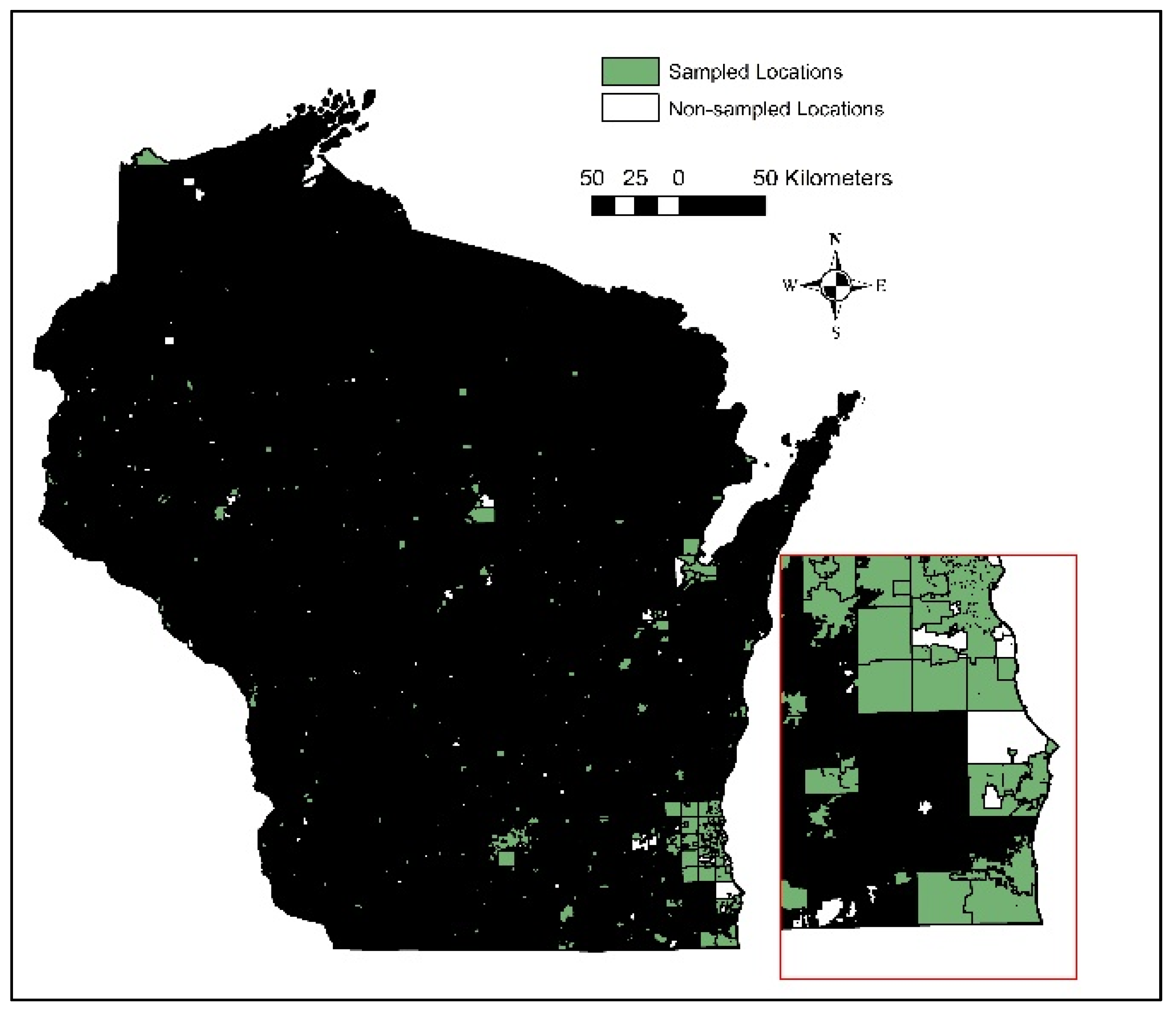
2.1. Study Site

The study occurred in Wisconsin, USA and used census designated places (which are defined as a community in this study) throughout the state as sample locations (Figure 1) [55,56]. The state has approximately 5.9 million inhabitants and 17 million hectares of total landcover [55]. A sample of 404 communities were selected from a total of 685 cities (191), villages (411), and towns (83) in the state [56]. The study locations were selected based on communities that participated in a 2017 study that detailed what urban forestry activities they undertake [57], as well as on the availability of aerial imagery for creating a UTC assessment. Communities, mainly towns, which lacked aerial imagery or AI-derived landcover were excluded from the study. The sampled community populations ranged from 75 to 584,000 people.

2.2. Tree Canopy Cover Estimation Process

Estimates of UTC through HI used aerial imagery acquired from the National Agriculture Imagery Program (NAIP). The NAIP images were leaf-on for both 2013 and 2018 and 1 m resolution [58]. The study dates were selected based on available NAIP imagery in 2013 and 2018. The 2013 imagery was the base for comparison to an AI system by Erker et al. [41]. Community boundary data for the selected sample communities were obtained from the Wisconsin Department of Natural Resources (WIDNR) Forestry GIS repository [55]. Each community had 1000 randomly placed sample points which were used to estimate UTC, using the Create Random Points tool in ArcMap 10.8.1 (ESRI, Redlands, CA, USA) using methods of Hilbert et al. [17]. Each point was identified as fitting within one of seven assessed landcover classifications used in the AI study. These classifications included (1) agriculture, (2) herbaceous and grass, (3) impervious, (4) soil, (5) tree and shrub, (6) water, and (7) wetland. The tree and shrub classification are also defined as UTC to calculate total % UTC in the results. A team of eight assessors collectively classified communities for both time periods, with images randomly assigned to each assessor. A training session was used to calibrate assessors for a consensus on which landcover classification a sample point was located over. To determine the landcover for the HI, an assessor would zoom into each random point at a scale of 1:1600 or greater magnification of up to 1:800 to classify the location using the center of the sample point (a circle with cross hairs). For each community, the points for each landcover classification category were summed and divided by 1000 points. This number was then multiplied by 100 to convert to a percentage of the total landcover for that location. The process was performed in both 2013 and 2018 to analyze the change in landcover between the 5-year interval for each community.

2.3. Tree Canopy Cover Comparison Process

Results from 2013 HI estimates were compared against AI estimates for 2013 for communities throughout the state [41]. To be consistent with the AI approach, the impervious and soil classification were summed together within an impervious classification unit. Agriculture was also combined with the herbaceous and grass. This resulted in five categories (herbaceous and grass, impervious and soil, tree and shrub, water, and wetland) used in the AI system [41]. The AI-generated estimates for each community used data from: (https://dnr.wisconsin.gov/topic/urbanforests/ufia/landcover (WIDNR Wisconsin Community Canopy Cover, accessed on 16 December 2022) derived from Erker et al. [41]. The AI system did not classify water and wetland; they were derived from vector layers provided by the WIDNR.

2.4. Accuracy Assessment for Human Intelligence Estimates

Two assessors classified a random 10 % sample (100 points per map) of HI points for each community using both 2013 and 2018 imagery to test for assessment accuracy using the same landcover classifications. The ArcMap 10.8.1 Create Random Points function was used to select the random sample for cross validation. The Assessors Agreement explains how many points within a landcover classification that both assessors agreed upon relative to points they classified in a landcover classification. The approach was calculated as follows:
Assessors Agreement: (Total Agreement/Mean Sample Points) ∗ 100
Total Agreement was the number of sample points that the 1st Assessor and 2nd Assessor agreed upon within a classification. Mean Sample Points was the mean number of sample points that the 1st Assessor and 2nd Assessor evaluated within a classification. For example, the Assessors had total agreement for 86 sample points in a landcover classification that combined they had had 180 points (Mean Sample Points = 90; 88 for Assessor 1 and 92 for Assessor 2):
Assessors Agreement: (86 ⁄ 90) ∗ 100 = 95.6%

2.5. Statistical Approach

We used SPSS Version 28 (IBM Corp, Armonk, NY, USA) for statistical analysis. A paired t-test was used to compare the estimates of each landcover classification from AI and HI methods using data from all communities (n = 397) statewide. A paired t-test was also used to evaluate for the difference between the HI and AI methods in the location (Dane County, WI, USA) used to train the AI system (n = 21). Similarly, a paired t-test was used to test for differences in landcover classification estimates between two time periods (2013–2018) and percent change in each landcover classification (n = 404). An ANOVA was used to test for assessor agreement. For this study, an α ≤ 0.05 was used for decision-making to interpret differences. A standard error of the mean (SEM) was further calculated for the interpretation of the findings.

3. Results

This study found differences in the UTC classification between AI and HI for communities outside the training location. However, no difference was found between the AI and the HI within the training location for UTC. The HI system also showed a change in landcover between the years of 2013 and 2018 with the percentage of UTC increasing. Lastly, assessor agreements for the HI were between 90% and 95% for UTC.

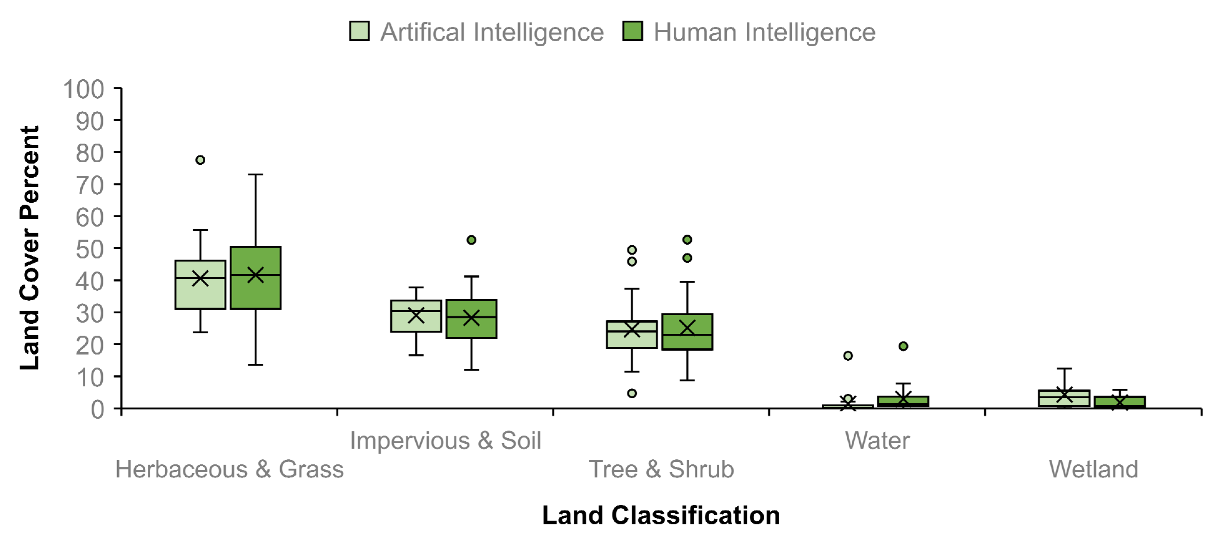
3.1. HI vs. AI Using Training Location Imagery

No difference was found within the training location between the HI and AI for UTC estimates (p = 0.723). Additionally, no difference was found for the herbaceous and grass (p = 0.332) and impervious (p = 0.218) landcover classifications for the training location (Table 1). Differences were found with water (p = 0.003) and wetland (p = 0.006). Both water and wetland were uncommon and each below approximately 4% overall of total land cover for the communities studied. Herbaceous was most common with approximately more than 41% of overall land cover. Both impervious and soil and trees and shrubs each comprised approximately one-quarter of the overall landcover for the 21 studied communities in the Dane County, WI, USA region training location (Figure 2).

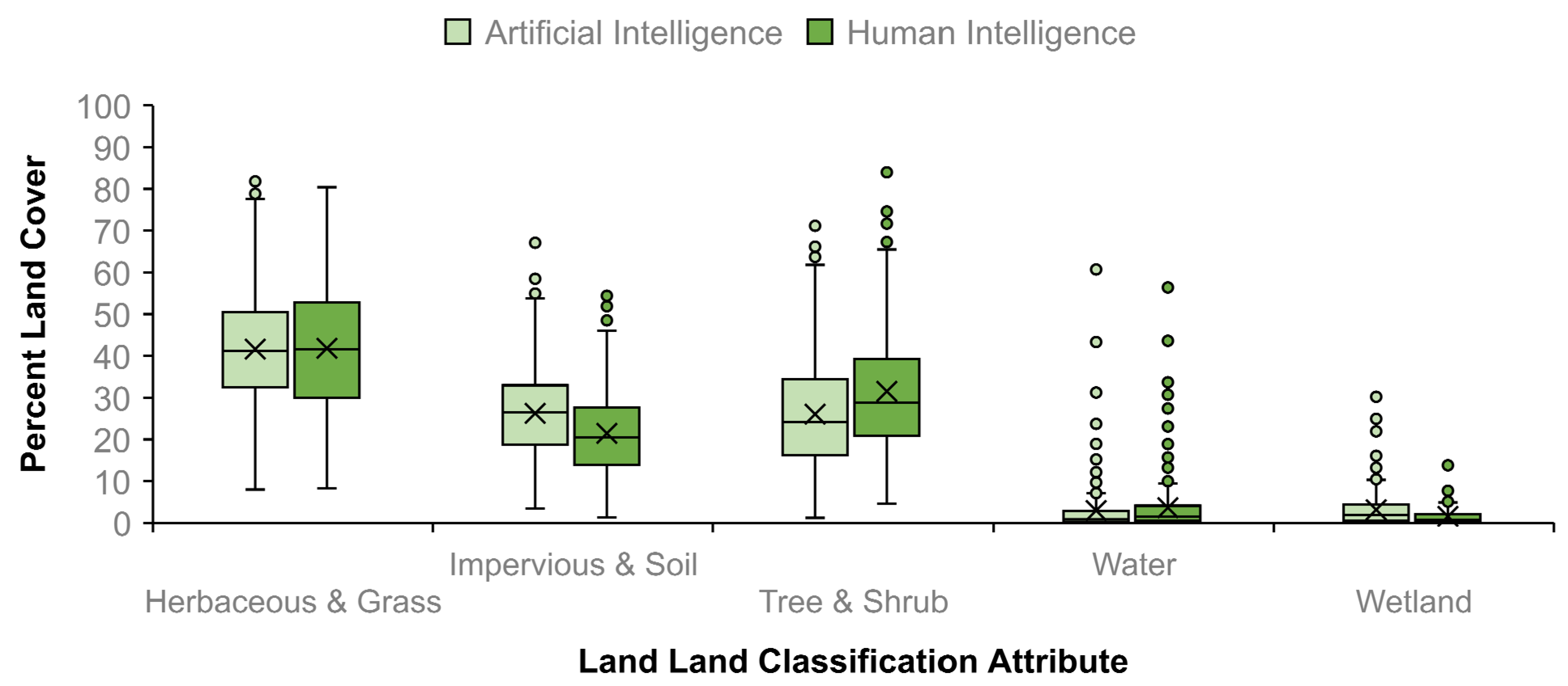
3.2. HI vs. AI Using Statewide Imagery

A difference was found between the HI and AI systems when land classifications were conducted beyond the AI training area were included. Four landcover classifications (impervious and soil, trees and shrubs, water, and wetland) significantly differed (p < 0.001) between HI and AI systems (Table 2). No difference (p = 0.743) occurred for the herbaceous category. The herbaceous landcover classification was most common for both systems (~42%). The tree and shrub estimate was higher for the HI (31.5%, SE = 0.72) than in AI (26.0%, SE = 0.72). In contrast, the impervious and soil classification was higher for the AI (26.2%, SE = 0.53) than in HI (21.5 %, SE = 0.51). Both wetland and water classifications each covered a small area, below 4% overall (Figure 3).

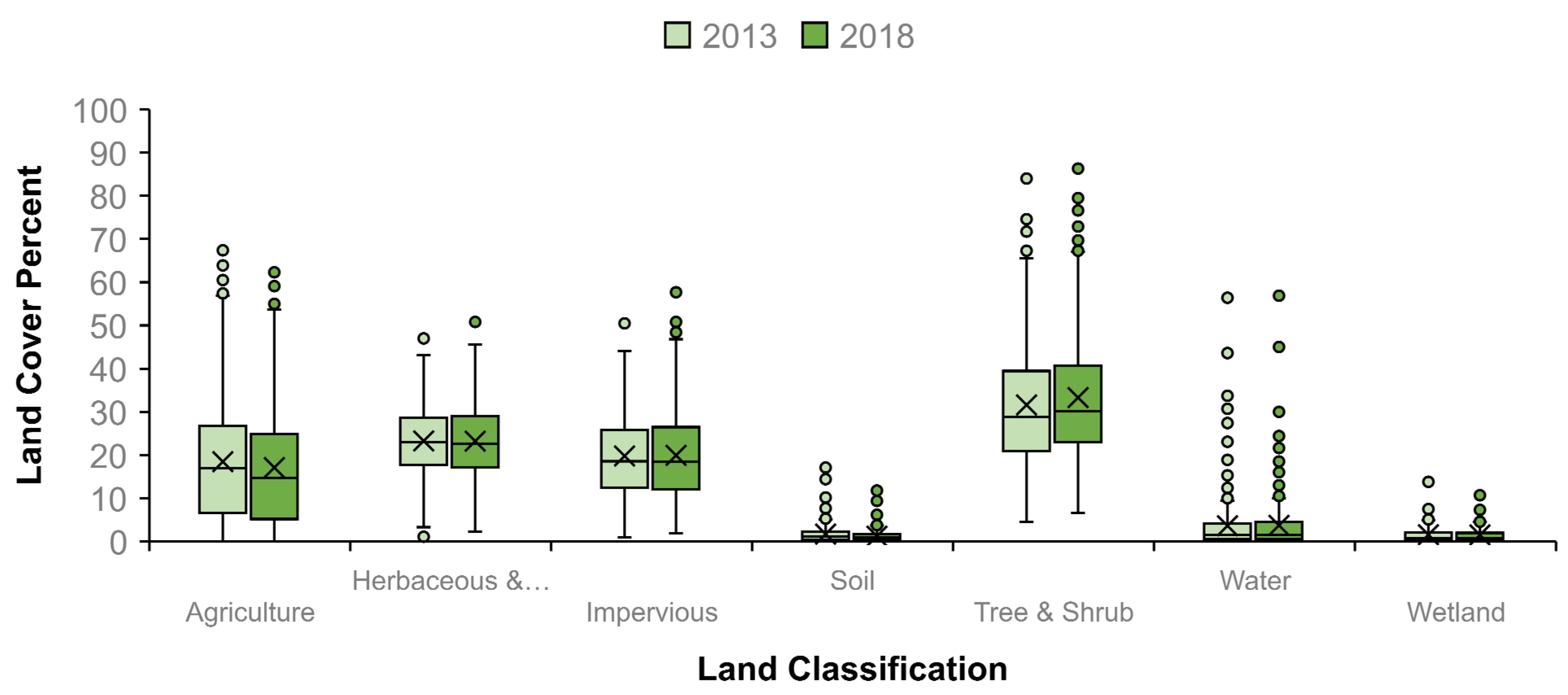
3.3. Comparison between 2013 and 2018 Using HI Method

Three of the seven land classifications significantly changed (p < 0.001) between 2013 and 2018 (Table 3, Figure 4). The tree-and-shrub-based UTC increased by 1.73% (0.17 SEM) from 31.6% (2013) to 33.3% (2018). Decreases occurred for soil (0.47%, 0.08 SEM) and agriculture (1.38%, 0.17 SEM). Water increased (p = 0.043) by 0.11% (0.06 SEM).
The UTC varied between 4.4% and 84.0% for communities in 2013. In 2018 the range was 6.8% to 86.3%. Tree cover was the most common classification for both 2013 (31.6%) and 2018 (33.3%). Herbaceous and grass were the next most common in 2013 (23.3%) and 2018 (23.2%). Impervious area was unchanged (p = 0.242) between the two time periods, 2013 (19.8%) and 2018 (19.9%). Agriculture decreased (p < 0.001) from 18.5% in 2013 to 17.1% in 2018. Soil, water, and wetland were all relatively uncommon, each below 5%.

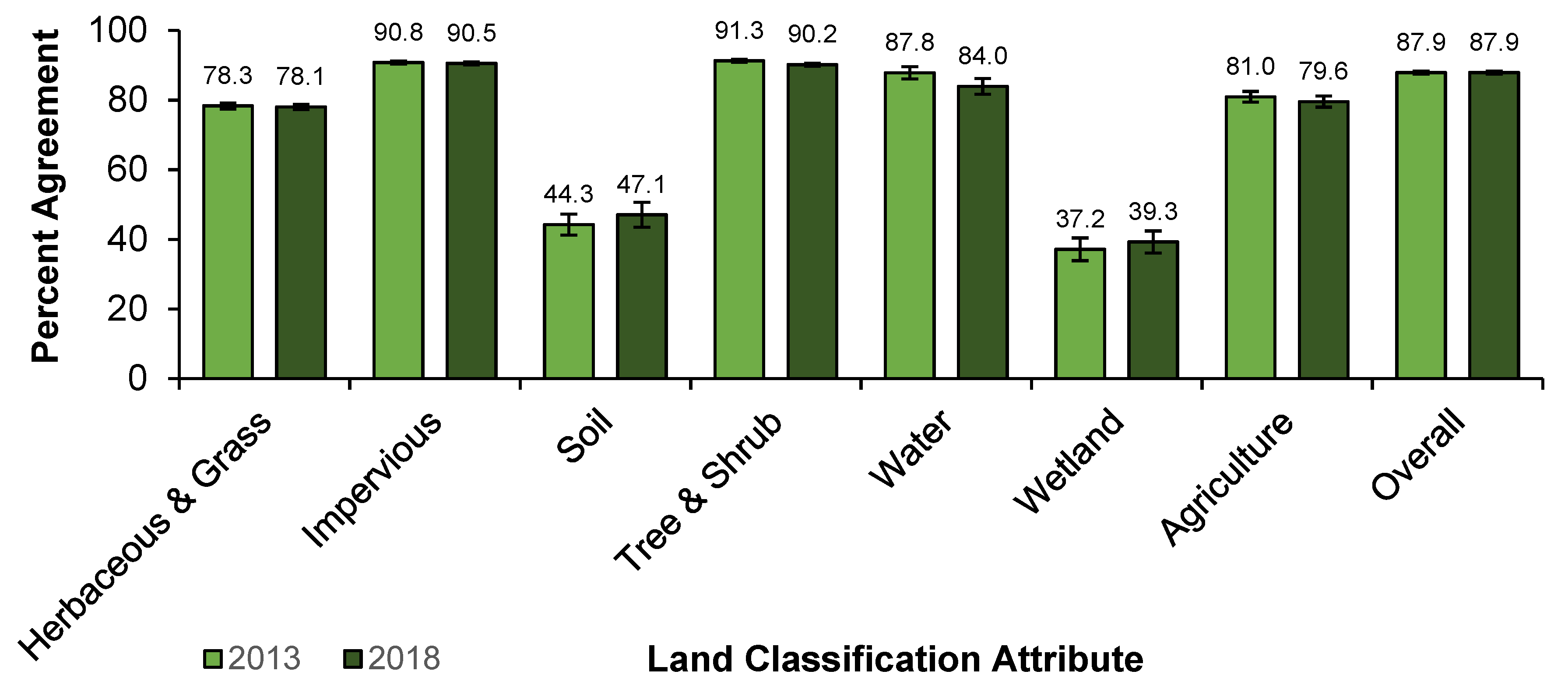
3.4. Assessor and Land Class Agreement

The assessor’s agreement showed no significant difference (p = 0.990) between assessors, or between 2013 and 2018 (p = 0.725). However, significant difference (p < 0.001) occurred for the wetland (<40% agreement) and soil (<50%) classifications (Figure 5). Agreement with impervious and tree and shrub were highest and exceeded 90%. Overall, for all landcover classifications during both periods an 87.9% agreement occurred (Figure 5).

4. Discussion

4.1. HI vs. AI Using Training Location Imagery

The study showed no significant difference between AI and HI in the training location for terrestrial land covers. This finding is consistent with the results of Erker et al. [41], who found no difference between their AI estimates and estimated UTC using a random point sample method. That approach is the same as we used for our HI method. Thus, this provides evidence supporting the AI estimates from the Erker [41] method in the training location. Water and wetland land classes were significantly different between the AI and HI systems. However, these aquatic features were derived from a data source independent of the imagery used to estimate landcover classifications in the AI [41].

4.2. HI vs. AI Using Statewide Imagery

The statewide comparison between HI and AI were significantly different for all land cover classifications except herbaceous. The interpretation methods may differ due to inconsistencies in the AI algorithm, shadows, differing tree heights, as well as change in tree community structure (e.g., northern Wisconsin is more coniferous) by location [41]. Common misclassifications with AI systems may also be related to pixels occurring on the edge of vegetated and non-vegetated areas, and spectral similarities between certain landcover classification types [54]. The AI might misclassify UTC in areas that have mixed-use landcover compared to urban and agricultural areas [39].
There are reasons that explain AI challenges to identify UTC and non-represented training data may be a factor. A change in forest structure, phenology, and composition from the training location may decrease the accuracy of the AI [59]. If the canopy structure changes due to different tree species, the AI might not be able to identify trees correctly, as coniferous and deciduous trees can have a spectral reflectance difference [59,60,61]. Likewise, weather-driven differences across a region may lead to different spectral signatures for the same species (e.g., because of drought). It is important to train AI to represent the variability present in landcover types that will be assessed [60]. This is especially true if the assessment area is large and has differing landcover and geography throughout. Additionally, it is important to take into consideration that there are different methods of assessing UTC as well as data sources of varying scales, qualities, and time periods [11,59,60,61,62,63,64]. For example, an AI method [41] that used NAIP imagery provided much higher levels of accuracy for UTC estimations than SPOT imagery [41]. Thus, there are many AI methods and algorithms that would impact the final product as well.

4.3. Comparison between 2013 and 2018 Using HI Method

The UTC in 2018 from this study was approximately 33.3% based on the HI assessment, while Nowak and Greenfield [65] used a similar methodology to this study and reported a mean 38.3 % (1.5 SE) UTC from 2015 data in Wisconsin. Differences between these two estimates can be attributed to Nowak and Greenfield [65] excluding water bodies (~4% in Wisconsin communities), fewer sample points (1000) versus much greater (~800,000) from this study, and different geographies (they included Census-defined urban areas and Census-designated places). Although the tree canopy increased overall, some communities experienced a local loss of UTC which may be due to pests such as emerald ash borer [66], storms [36], or urbanization [32].
The UTC in Wisconsin increased significantly between 2013 and 2018. Unlike locations in the conterminous United States, which experienced a 0.2% annual UTC loss, Wisconsin’s UTC has increased by almost 2% in the five-year interval studied [31,65]. The UTC increased, while agricultural landcover decreased over the 5-year period. Agricultural landcover area has decreased in some conterminous United States regions, while urbanized area has increased [66]. Areas that transition from agricultural landcover to urban or suburban may experience an increase in UTC [64], although there are some locations such as Detroit, Michigan where urbanized areas are in decline and agricultural areas are increasing [67].

4.4. Assessor and Land Class Agreement

Another assessor validated the HI interpretation. It is important to assess agreement of the first assessor as a form of quality control [8]. Both the soil and wetland classifications had the highest level of disagreement, which might be in part due to the low percent of landcover overall that is made up of these two landcover types. However, water also comprised a low overall percentage of sample points and two assessors readily agreed on this landcover classification. As the number of sample points for a landcover increases, error declines [6,8]. Error in assessments may also be related to aerial imagery quality [47,48]. Thus, it is more likely that estimating soil and wetland is currently a challenge and improved methods are needed for soil and wetland interpretation. Further, the sampling intensity (e.g., number of sample points) is a function of the area covered by a landcover attribute and a pre-sampling estimate can be used to determine the sampling point intensity.
The overall agreement for UTC was between 90% and 95% for 2013 and 2018 which is consistent with other current UTC studies [8,17]. The agreement between assessors for the study in Florida ranged from 94.9% to 99.5% [17]. The higher levels of accuracy in Florida are most likely due to the classification system of tree or not tree compared to seven different landcover types in this study. These high levels of agreement reinforce the accuracy of HI assessments in this study between two assessors using an HI approach.

5. Conclusions

We created an HI assessment of landcover specifically with UTC to compare to AI estimates. We found a significant difference in UTC between the two methods for those for communities outside the training location. However, we found that there was no difference in UTC in the training location of the AI. Findings from this study could aid in understanding how AI canopy assessment performs outside of its training locations to improve AI development. Future research could include appropriate sampling and training in multiple locations to aid in higher accuracy levels for the AI system. We also compared HI between 2013 and 2018 and found an increase in UTC. The availability of high-resolution imagery and the implementation of UTC goals whether statewide or by municipality have created an increase in research related to urban forest land cover. Research comparing canopy assessments using AI to HI methods is limited, especially on a statewide scale [6]. These comparison analyses will provide insight into the most accurate and beneficial UTC assessments. Understanding the UTC and, therefore, urban forest is crucial for appropriate management and improved policies.

Author Contributions

Conceptualization: E.F.C.-S., D.R.H., D.B. and R.J.H.; methodology: E.F.C.-S. and D.R.H.; validation: D.R.H.; formal analysis: E.F.C.-S. and R.J.H.; investigation: E.F.C.-S. and R.J.H.; resources: E.F.C.-S. and R.J.H.; data curation: R.J.H.; writing—original draft preparation: E.F.C.-S. and R.J.H.; writing—review and editing: R.J.H., D.R.H., A.K.K., D.B., L.B., E.L., N.T. and L.P.W.; visualization: E.F.C.-S. and R.J.H.; supervision: R.J.H.; project administration: E.F.C.-S. and R.J.H.; funding acquisition: R.J.H. and L.B.; All authors have read and agreed to the published version of the manuscript.

Funding

This research was funded by the Wisconsin Department of Natural Resources, USFS grant award 19-DG-114200004-094. This work was supported by the USDA National Institute of Food and Agriculture, McIntire–Stennis project 1021277 and the University of Wisconsin—Stevens Point. Financial support also occurred through Wisconsin Consortium for Extension and Research in Agriculture and Natural Resources (CERANR) STP100239.

Data Availability Statement

Data potentially available upon request.

Acknowledgments

The authors would like to thank Emily Cleaver, Bowen Li, Jeremy Natzke, and Matthew Johns for their technical support.

Conflicts of Interest

The authors declare no conflict of interest.

References

  1. Roy, S.; Byrne, J.; Pickering, C. A systematic quantitative review of urban tree benefits, costs, and assessment methods across cities in different climatic zones. Urban For. Urban Green. 2012, 11, 351–363. [Google Scholar] [CrossRef] [Green Version]
  2. Nowak, D.; Appleton, N.; Ellis, A.; Greenfield, E. Residential building energy conservation and avoided power plant emissions by urban and community trees in the United States. Urban For. Urban Green. 2017, 21, 158–165. [Google Scholar] [CrossRef] [Green Version]
  3. Lin, J.; Kroll, C.; Nowak, D.; Greenfield, E. A review of Urban Forest Modeling: Implications for Management and Future Research. Urban For. Urban Green. 2019, 43, 126366. [Google Scholar] [CrossRef]
  4. Jennings, S. Assessing forest canopies and understorey illumination: Canopy closure, canopy cover and other measures. Forestry 1999, 72, 59–74. [Google Scholar] [CrossRef]
  5. King, K.; Locke, D. A comparison of three methods for measuring local urban tree canopy cover. Arboric Urban For. 2013, 39, 62–67. [Google Scholar] [CrossRef]
  6. Locke, D.; Romolini, M.; Galvin, M.; O’Neil-Dunne, J.; Strauss, E. Tree canopy change in coastal Los Angeles, 2009–2014. Cities Environ. 2017, 10, 3. [Google Scholar]
  7. Hermansen-Baez, A. Urban Tree Canopy Assessment: A Community’s Path to Understanding and Managing the Urban Forest; FS-1121; U.S. Department of Agriculture: Washington, DC, USA, 2019. [Google Scholar]
  8. Parmehr, E.; Amati, M.; Taylor, E.; Livesley, S. Estimation of urban tree canopy cover using random point sampling and remote sensing methods. Urban For. Urban Green. 2016, 20, 160–171. [Google Scholar] [CrossRef]
  9. Nowak, D.; Crane, D.; Stevens, J.; Hoehn, R.; Walton, J.; Bond, J. A ground-based method of assessing urban forest structure and Ecosystem Services. Arboric Urban For. 2008, 34, 347–358. [Google Scholar] [CrossRef]
  10. Timilsina, S.; Aryal, J.; Kirkpatrick, J. Mapping urban tree cover changes using object-based convolution neural network (OB-CNN). Remote Sens. 2020, 12, 3017. [Google Scholar] [CrossRef]
  11. Nowak, D.J.; Rowntree, R.A.; McPherson, E.; Sisinni, S.; Kerkmann, E.; Stevens, J. Measuring and analyzing urban tree cover. Landsc. Urban Plan. 1996, 36, 49–57. [Google Scholar] [CrossRef] [Green Version]
  12. Chuang, W.; Boone, C.; Locke, D.; Grove, J.; Whitmer, A.; Buckley, G.; Zhang, S. Tree canopy change, and neighborhood stability: A comparative analysis of Washington, DC and Baltimore, MD. Urban For. Urban Green. 2017, 27, 363–372. [Google Scholar] [CrossRef]
  13. Berland, A. Long-term urbanization effects on tree canopy cover along an urban rural gradient. Urban Ecosyst. 2012, 15, 721–738. [Google Scholar] [CrossRef]
  14. Baines, O.; Wilkes, P.; Disney, M. Quantifying urban forest structure with open-access remote sensing data sets. Urban For. Urban Green. 2020, 50, 126653. [Google Scholar] [CrossRef]
  15. Hostetler, A.; Rogan, J.; Martin, D.; DeLauer, V.; O’Neil-Dunne, J. Characterizing tree canopy loss using multi-source GIS data in Central Massachusetts, USA. Remote Sens. Lett. 2013, 4, 1137–1146. [Google Scholar] [CrossRef]
  16. McPherson, G.; Simpson, J.; Xiao, Q.; Chunxia, W. Los Angeles 1-Million Tree Canopy Cover Assessment; USDA-FS; U.S. Department of Agriculture: Albany, CA, USA; Forest Service: Albany, CA, USA; Pacific Southwest Research Station: Albany, CA, USA, 2008. [Google Scholar]
  17. Hilbert, D.; Koeser, A.; Roman, L.; Hamilton, K.; Landry, S.; Hauer, R.; Campanella, H.; McLean, D.; Andreu, M.; Perez, H. Development practices and ordinances predict inter-city variation in Florida urban tree canopy coverage. Landsc. Urban Plan. 2019, 190, 103603. [Google Scholar] [CrossRef]
  18. Ren, Z.; Du, Y.; He, X.; Pu, R.; Zheng, H.; Hu, H. Spatiotemporal pattern of Urban Forest Leaf Area Index in response to rapid urbanization and Urban Greening. J. For. Res. 2017, 29, 785–796. [Google Scholar] [CrossRef]
  19. Salisbury, A.; Koeser, A.; Hauer, R.; Hilbert, D.; Abd-Elrahman, A.; Andreu, M.; Britt, K.; Landry, S.; Lusk, M.; Miesbauer, J.; et al. The Legacy of Hurricanes, Historic Land Cover, and Municipal Ordinances on Urban Tree Canopy in Florida (United States). Front. For. Glob. Change 2022, 5, 742157. [Google Scholar] [CrossRef]
  20. Hauer, R.; Timilsina, N.; Vogt, J.; Fischer, B.; Wirtz, Z.; Peterson, W. A volunteer and partnership baseline for municipal forestry activity in the United States. Arboric Urban For. 2018, 44, 87–100. [Google Scholar] [CrossRef]
  21. Hauer, R.; Koeser, A.; Parbs, S.; Kringer, J.; Krouse, R.; Ottman, K.; Miller, R.; Sivyer, D.; Timilsina, N.; Werner, L. Long-term effects and development of a tree preservation program on tree condition, survival, and growth. Landsc. Urban Plan. 2020, 193, 103670. [Google Scholar] [CrossRef]
  22. Roman, L.; Battles, J.; McBride, J. Determinants of establishment survival for residential trees in Sacramento County, CA. Landsc. Urban Plan. 2014, 129, 22–31. [Google Scholar] [CrossRef]
  23. Nowak, D.; Hoehn, R.; Bodine, A.; Greenfield, E.; O’Neil-Dunne, J. Urban forest structure, ecosystem services and change in Syracuse, NY. Urban Ecosyst. 2016, 19, 1455–1477. [Google Scholar] [CrossRef]
  24. Roman, L.; Pearsall, H.; Eisenman, T.; Conway, T.; Fahey, R.; Landry, S.; Vogt, J.; van Doorn, N.; Grove, J.; Locke, D.; et al. Human and biophysical legacies shape contemporary urban forests: A literature synthesis. Urban For. Urban Green. 2018, 31, 157–168. [Google Scholar] [CrossRef]
  25. Riley, C.; Gardiner, M. Examining the distributional equity of urban tree canopy cover and ecosystem service across United States cities. PLoS ONE 2020, 15, e0230398. [Google Scholar] [CrossRef] [PubMed] [Green Version]
  26. Turner-Skoff, J.; Cavender, N. The benefits of trees for livable and sustainable communities. Plants People Planet 2019, 1, 323–335. [Google Scholar] [CrossRef]
  27. Lowry, J.; Baker, M.; Ramsey, R. Determinants of urban tree canopy in residential neighborhoods: Household characteristics, urban form, and the Geophysical Landscape. Urban Ecosyst. 2011, 15, 247–266. [Google Scholar] [CrossRef]
  28. Danford, R.; Cheng, C.; Strohbach, M.; Ryan, R.; Nicolson, C.; Warren, P. What does it take to achieve equitable urban tree canopy distribution? A Boston case study. PLoS ONE 2020, 15, e0230398. [Google Scholar]
  29. Schwarz, K.; Fragkias, M.; Boone, C.; Zhou, W.; McHale, M.; Grove, J.; O’Neil-Dunne, J.; McFadden, J.; Buckley, G.; Childers, D.; et al. Trees Grow on Money: Urban Tree Canopy Cover and Environmental Justice. PLoS ONE 2015, 10, e0122051. [Google Scholar] [CrossRef] [Green Version]
  30. Troy, A.; Morgan Grove, J.; O’Neil-Dunne, J. The relationship between tree canopy and crime rates across an urban–rural gradient in the greater Baltimore region. Landsc. Urban Plan. 2012, 106, 262–270. [Google Scholar] [CrossRef]
  31. Nowak, D.; Greenfield, E. Tree and impervious cover change in U.S. cities. Urban For. Urban Green. 2012, 11, 21–30. [Google Scholar] [CrossRef] [Green Version]
  32. Nowak, D.; Greenfield, E. The increase of impervious cover and decrease of tree cover within urban areas globally (2012–2017). Urban For. Urban Green. 2020, 49, 126638. [Google Scholar] [CrossRef]
  33. Hill, E.; Dorfman, J.; Kramer, E. Evaluating the impact of government land use policies on tree canopy coverage. Land Use Policy 2010, 27, 407–414. [Google Scholar] [CrossRef] [Green Version]
  34. Hauer, R.; Hanou, I.; Sivyer, D. Planning for active management of future invasive pests affecting urban forests: The ecological and economic effects of varying Dutch elm disease management practices for street trees in Milwaukee, WI USA. Urban Ecosyst. 2020, 23, 1005–1022. [Google Scholar] [CrossRef]
  35. Hauer, R.; Johnson, G.; Kilgore, M. Local outcomes of Federal and State Urban; Community Forestry Programs. Arboric. Urban For. 2011, 37, 152–159. [Google Scholar] [CrossRef]
  36. Rahman, M.; Rashed, T. Urban tree damage estimation using airborne laser scanner data and geographic information systems: An example from 2007 Oklahoma Ice Storm. Urban For. Urban Green. 2015, 14, 562–572. [Google Scholar] [CrossRef]
  37. Blackman, R.; Yuan, F. Detecting long-term urban forest cover change and impacts of natural disasters using high-resolution aerial images and Lidar Data. Remote Sens. 2020, 12, 1820. [Google Scholar] [CrossRef]
  38. Dwyer, M.; Miller, R. Using GIS to assess urban tree canopy benefits and surrounding greenspace distributions. Arboric. Urban For. 1999, 25, 102–107. [Google Scholar] [CrossRef]
  39. Pregitzer, C.; Ashton, M.; Charlop-Powers, S.; D’Amato, A.; Frey, B.; Gunther, B.; Hallett, R.; Pregitzer, K.; Woodall, C.; Bradford, M. Defining and assessing urban forests to inform management and policy. Environ. Res. Lett. 2019, 14, 085002. [Google Scholar] [CrossRef]
  40. Mullins, R.; Fargo, H. Protecting and Developing the Urban Tree Canopy: A 135-City Survey. In Proceedings of the United States Conference of Mayors, Washington, DC, USA, 18–20 October 2008; pp. 7–19. [Google Scholar]
  41. Erker, T.; Wang, L.; Lorentz, L.; Stoltman, A.; Townsend, P. A statewide urban tree canopy mapping method. Remote Sens. Environ. 2019, 229, 148–158. [Google Scholar] [CrossRef]
  42. Wang, Z.; Fan, C.; Xian, M. Application and evaluation of a deep learning architecture to urban tree canopy mapping. Remote Sens. 2021, 13, 1749. [Google Scholar] [CrossRef]
  43. Moskal, L.; Styers, D.; Halabisky, M. Monitoring urban tree cover using object-based image analysis and public domain remotely sensed data. Remote Sens. 2011, 3, 2243–2262. [Google Scholar] [CrossRef] [Green Version]
  44. Korteling, J.; van de Boer-Visschedijk, G.; Blankendaal, R.; Boonekamp, R.; Eikelboom, A. Human- versus Artificial Intelligence. Front. Artif. Intell. 2021, 4, 622364. [Google Scholar] [CrossRef] [PubMed]
  45. Hanssen, F.; Barton, D.; Venter, Z.; Nowell, M.; Cimburova, Z. Utilizing LiDAR data to map tree canopy for urban ecosystem extent and condition accounts in Oslo. Ecol. Indic. 2021, 130, 108007. [Google Scholar] [CrossRef]
  46. Pristeri, G.; Peroni, F.; Pappalardo, S.; Codato, D.; Masi, A.; De Marchi, M. Whose urban green? mapping and classifying public and private green spaces in Padua for spatial planning policies. ISPRS Int. J. Geo-Inf. 2021, 10, 538. [Google Scholar] [CrossRef]
  47. Alonzo, M.; Bookhagen, B.; Roberts, D. Urban Tree Species Mapping using hyperspectral and Lidar Data Fusion. Remote Sens. Environ. 2014, 148, 70–83. [Google Scholar] [CrossRef]
  48. Al-Kofahi, S.; Steele, C.; VanLeeuwen, D.; Hilaire, R.S. Mapping land cover in urban residential landscapes using very high spatial resolution aerial photographs. Urban For. Urban Green. 2012, 11, 291–301. [Google Scholar] [CrossRef]
  49. Cleve, C.; Kelly, M.; Kearns, F.; Moritz, M. Classification of the wildland–urban interface: A comparison of pixel- and object-based classifications using high-resolution aerial photography. Comput. Environ. Urban. Syst. 2008, 32, 317–326. [Google Scholar] [CrossRef]
  50. MacFaden, S.; O’Neil-Dunne, J.; Royar, M.; Lu, A.; Rundle, A. High-resolution tree canopy mapping for New York City using LIDAR and object-based image analysis. J. Appl. Remote Sens. 2012, 6, 063567. [Google Scholar] [CrossRef]
  51. Walker, J.; Briggs, J. An object-oriented approach to urban forest mapping in Phoenix. Photogramm. Eng. Remote Sens. 2007, 73, 577–583. [Google Scholar] [CrossRef]
  52. Zhou, W.; Troy, A. An object-oriented approach for analysing and characterizing urban landscape at the parcel level. Int. J. Remote Sens. 2008, 29, 3119–3135. [Google Scholar] [CrossRef]
  53. Ellis, E.; Mathews, A. Object-based delineation of urban tree canopy: Assessing change in Oklahoma City, 2006–2013. Comput. Environ. Urban. Syst. 2019, 73, 85–94. [Google Scholar] [CrossRef]
  54. He, D.; Shi, Q.; Liu, X.; Zhong, Y.; Zhang, L. Generating 2m fine-scale urban tree cover product over 34 metropolises in China based on deep context-aware sub-pixel mapping network. Int. J. Appl. Earth Obs. Geoinf. 2022, 106, 102667. [Google Scholar] [CrossRef]
  55. Wisconsin Department of Natural Resources Forestry GIS Data. Available online: https://dnr.wisconsin.gov/topic/forestmanagement/data (accessed on 4 April 2022).
  56. Bureau, U.S.C. City and Town Population Totals: 2010–2019. Available online: https://www.census.gov/data/tables/time-series/demo/popest/2010s-total-cities-and-towns.html (accessed on 9 April 2022).
  57. Hauer, R.; Lorentz, L. Trees in Your Community 2018: Results from a 2017 Questionnaire for the Urban Forestry Program. Available online: https://dnr.wisconsin.gov/sites/default/files/topic/UrbanForests/treesInYourCommunity.pdf (accessed on 4 April 2022).
  58. National Agriculture Imagery Program (NAIP). Available online: https://naip-usdaonline.hub.arcgis.com/ (accessed on 1 December 2022).
  59. Myeong, S.; Nowak, D.; Hopkins, P.; Brock, R. Urban cover mapping using digital, high-spatial resolution aerial imagery. Urban Ecosyst. 2001, 5, 243–256. [Google Scholar] [CrossRef]
  60. Shanmugam, P.; Ahn, Y.; Sanjeevi, S. A comparison of the classification of wetland characteristics by linear spectral mixture modelling and traditional hard classifiers on multispectral remotely sensed imagery in southern India. Ecol. Model. 2006, 194, 379–394. [Google Scholar] [CrossRef]
  61. Cipar, J.; Cooley, T.; Lockwood, R.; Grigsby, P. Distinguishing between coniferous and deciduous forests using hyperspectral imagery. In Geoscience and Remote Sens. Symposium, Proceedings of the 2004 IEEE International Geoscience and Re-mote Sensing Symposium, Anchorage, AK, USA, 20–24 September 2004; Volume 4, pp. 2348–2351. [Google Scholar]
  62. Rautiainen, M.; Lukeš, P.; Homolová, L.; Hovi, A.; Pisek, J.; Mõttus, M. Spectral Properties of Coniferous Forests: A Review of In Situ and Laboratory Measurements. Remote Sens. 2018, 10, 207. [Google Scholar] [CrossRef] [Green Version]
  63. Brown, J.; Tollerud, H.; Barber, C.; Zhou, Q.; Dwyer, J.; Vogelmann, J.; Loveland, T.; Woodcock, C.; Stehman, S.; Zhu, Z.; et al. Lessons learned implementing an operational continuous United States national land change monitoring capability: The land change monitoring, assessment, and projection (LCMAP) approach. Remote Sens. Environ. 2020, 238, 111356. [Google Scholar] [CrossRef]
  64. Coulston, J.; Moisen, G.; Wilson, B.; Finco, M.; Cohen, W.; Brewer, C. Modeling percent tree canopy cover. Photogramm. Eng. Remote Sens. 2012, 78, 715–727. [Google Scholar] [CrossRef] [Green Version]
  65. Nowak, D.; Greenfield, E. US urban forest statistics, values, and projections. J. For. 2018, 116, 164–177. [Google Scholar] [CrossRef] [Green Version]
  66. Hauer, R.; Peterson, W. Effects of emerald ash borer on municipal forestry budgets. Landsc. Urban Plan. 2017, 157, 98–105. [Google Scholar] [CrossRef] [Green Version]
  67. Homer, C.; Dewitz, J.; Jin, S.; Xian, G.; Costello, C.; Danielson, P.; Gass, L.; Funk, M.; Wickham, J.; Stehman, S.; et al. Conterminous United States land cover change patterns 2001–2016 from the 2016 National Land Cover Database. ISPRS J. Photogramm. Remote Sens. 2020, 162, 184–199. [Google Scholar] [CrossRef]
Figure 1. Study locations throughout the state of Wisconsin USA where urban tree canopy was sampled (shaded green) compared to non-sampled locations (unshaded white). Milwaukee metropolitan (bottom right) expanded to show greater sample clarity.
Land 11 02325 g001
Figure 2. Landcover classification boxplot comparison between artificial intelligence and human intelligence in Dane County, WI, USA (n = 21). Only water and wetland were significantly different (p < 0.01). Box plots parts are lower box 1st quartile, line median, X mean, upper box 3rd quartile, line ends are minimum and maximum values, and circles are outliers.
Land 11 02325 g002
Figure 3. Landcover classification box plot comparison between artificial intelligence and human intelligence in WI, USA (n = 397). All location significantly different (p < 0.001) except for herbaceous (p = 0.743). Box plots parts are lower box 1st quartile, line median, X mean, upper box 3rd quartile, line ends are minimum and maximum values, and circles are outliers.
Land 11 02325 g003
Figure 4. Landcover classification box plot comparison between 2013 and 2018 in Wisconsin, USA. (n = 404). Box plots parts are lower box 1st quartile, line median, X mean, upper box 3rd quartile, line ends are minimum and maximum values, and circles are outliers.
Land 11 02325 g004
Figure 5. Assessors’ agreement for landcover classifications over two assessment time periods. (n = 404).
Land 11 02325 g005
Table 1. Comparison of percent estimates of different landcover classes using human intelligence (HI) and artificial intelligence (AI) in the AI training area (Dane County, WI, USA). n = 21.
Landcover ClassificationsHI
Mean
(%)
AI
Mean
(%)
Mean Difference = HI − AI (%)Standard Error of the Mean (%)95% Lower Confidence Interval95% Upper Confidence IntervalPaired t-Valuep-Value
Herbaceous and Grass42.6940.601.831.84−2.035.691.000.332
Impervious and Soil27.2629.04−1.401.10−3.700.90−1.280.218
Trees and Shrubs25.1724.660.431.19−2.072.920.360.723
Water2.941.461.480.430.572.383.420.003
Wetland1.944.24−2.340.75−3.91−0.77−3.130.006
Table 2. Mean landcover classification for human intelligence and artificial intelligence and their difference for communities in WI, USA using 2013 imagery. n = 397.
Landcover ClassificationsHI
Mean
(%)
AI Mean
(%)
Mean Difference = HI − AI (%)Standard Error of the Mean (%)95% Lower Confidence Interval95% Upper Confidence Intervalt-Valuep-Value
Herbaceous41.8341.640.180.56−0.921.290.330.743
Impervious and Soil21.4626.25−4.790.39−5.56−4.02−12.29<0.001
Trees and Shrubs31.5126.035.480.484.556.4111.54<0.001
Water3.642.940.700.100.500.906.90<0.001
Wetland1.573.14−1.570.18−1.921.22−8.88<0.001
Table 3. Landcover classification change between 2013 and 2018 in WI, USA. Percentages are based on human interpretation of NAIP aerial imagery. n = 404.
Landcover Classifications2013
Mean
(%)
2018 Mean
(%)
Mean
Change
(%)
Standard Error of the Mean (%)95% Lower Confidence Interval95% Upper Confidence IntervalPaired
t-Value
p-Value2
Agriculture18.4717.04−1.380.17−1.05−1.71 −8.17<0.001
Herbaceous and Grass23.2823.20−0.080.200.30−0.46−0.420.674
Impervious19.7819.910.130.110.34−0.091.170.242
Soil1.691.22−0.470.08−0.31−0.63−5.78<0.001
Trees and Shrubs31.5833.311.730.162.051.4110.73<0.001
Water3.643.750.110.060.220.002.030.043
Wetland1.561.52−0.040.060.09−0.17−0.620.539
Publisher’s Note: MDPI stays neutral with regard to jurisdictional claims in published maps and institutional affiliations.

