Quantifying the Impact of Urban Sprawl on Green Total Factor Productivity in China: Based on Satellite Observation Data and Spatial Econometric Models

Abstract

Worsening environmental effects caused by the rapid large-scale urban expansion in most Chinese cities is a worrying trend. In response, China is advocating an economic transition from rapid (raw growth) to a high-quality development model that incorporates negative environmental consequences. Green total factor productivity (GTFP) is regarded as one of the important approaches for measuring high-quality development. Hence, the aim of this research is to quantify the impact of urban sprawl on GTFP using remote sensing data and spatial econometric models. The primary findings of this study are as follows. (1) The urban sprawl index presents a decreasing trend from 2005 to 2016, indicating that urbanization has slowed; (2) The GTFP scores of Chinese cities are not randomly distributed and thus present significant spatial spillovers; and (3) The results of spatial lag models reveal that spatial spillover of GTFP is significant and positive. In other words, increases in GTFP in neighboring cities promotes GTFP improvements in nearby cities. We also find that the impact of urban sprawl on GTFP is significant and negative, indicating that rapid urban expansion is a contributor to decreased GTFP growth in China. Moreover, urban sprawl has a negative effect on technical change and efficiency change. The main findings can provide policy makers in Chinese cities with scientific foundations to design and implement effective measures to improve GTFP.

1. Introduction

China has achieved remarkable economic success and become the second largest economy in the world [1], due to the reform and opening-up policy initiated in 1978. Rapid urbanization has gone hand-in-hand with economic success, and has been the growth engine of the country [2]. Accordingly, China’s urbanization rate rapidly grew from 17.92% in 1978 to 63.89% in 2020 [3]. As opposed to Western developed countries, whose processes have lasted for more than a century, China’s urbanization process has taken place within a very short time. Urbanized China is primarily characterized by millions of urban dwellers and large areas of built-up regions [4]. Statistics show that the number of urbanites has quintupled, specifically, from 20,171 million in 1978 to 90,220 million in 2020. Moreover, the built-up areas in China have expanded from 6720 km² in 1981 to 60,721.3 km² in 2020 [5].

The rapid urban expansion in urbanizing China has not only driven economic growth [6], industrial upgrading [7], population agglomeration [8], and even climate change [9], but has also led to a series of adverse consequences, including massive encroachment onto agricultural land, the inability to utilize rural arable land resources, traffic congestion [10], serious environmental problems [11,12,13], and productivity losses [14]. As urban built-up areas have expanded, negative impacts and environmental vulnerability have subsequently increased [15].

For the past forty years, China has focused mainly on rapid economic growth that has been driven by industrialization and urbanization in a raw development model. As a consequence, it has achieved a remarkable milestone, becoming the second-largest economy in the world. However, the country’s rapid economic growth, with its long-term reliance on a resource-dependent growth model, has been accompanied by environmental decline, which not only impacts people’s health, but also delays sustainable development [16]. Hence, the Chinese central government has advocated an economic transition from raw growth to a high-quality development model [17], that is, the GDP growth target has been replaced by productivity and efficiency gains [18]. GTFP is presently regarded as a fundamental contributor to long-term sustainable economic growth [19]. Therefore, the GTFP, which is grounded in the traditional total factor productivity index, but also incorporates environmental pollutants as undesirable outputs and measures the ability of an economy to produce economic outputs while simultaneously minimizing adverse environmental consequences, has become the highest priority for local governments.

Since urban expansion has had a profoundly negative impact on Chinese cities in various ways, most notably regarding sustainable development, one may then ask whether urban sprawl in China has an explicit impact on GTFP. In the context of rapid urbanization in China, the answer to this question may not only contribute to optimizing urban spatial layout, but may also help us understand how urban form can reshape the economic activities of the cities and further affect GTFP. To this end, we used satellite remote sensing data to accurately quantify the levels of urban sprawl in Chinese cities, and then adopted a global Malmquist–Luenberger index approach to assess the GTFP score of each city. Lastly, we built a spatial econometric model to conduct an empirical investigation on the impact of urban sprawl on GTFP. The findings of this research may help policymakers assess the impact of urban spatial configuration changes on the realization of high-quality economic development targets.

2. Literature Review

2.1. Urban Sprawl

Urban sprawl has become a serious consequence of rapid urbanization [20]. There are many urban sprawl measurement methods, including single-indicator and multi-indicator methods. For example, Fulton et al. [21] used the population density as the urban sprawl index, where they pointed out that the lower the population density, the higher the level of urban sprawl. Kolankiewicz and Beck [22] adopted the growth of urban built-up areas to reflect urban sprawl levels, and found that the faster the growth of the urban built-up area, the higher the level of sprawl. Since the single-indicator method is not precise enough to quantify the level of urban sprawl, it is difficult to reflect the essence of urban sprawl comprehensively. Other studies have used statistical and survey data in their construction of multiple indicators to quantify urban sprawl, including measuring land use characteristics [23,24], population density, land use mix, degree of centering, and street accessibility [25], among others. However, the time periods of these statistical and survey data have been short, uncertainty has been high, and the time and labor spent have been too high, which all bring certain limitations to the traditional urban sprawl measurement methods [26]. Therefore, in recent years scholars have begun using remote sensing data and GIS techniques to measure urban sprawl [27,28,29]. Using DMSP/OLS nighttime light data, Gao et al. [30] monitored the urban sprawl in cities of varying sizes in China from 1990 to 2010; they found that the annual growth of urban areas was 2.45% larger than that of the urban population. Other relevant research conducted the urban sprawl scenario analysis in the Yangtze River Economic Belt in China [31], and identified the urban–rural fringes of megacities [32]. Chen et al. [33] considered both the horizontal sprawl (built-up area) and the vertical sprawl (population activity intensity or population density) to comprehensively measure urban sprawl in Chinese cities. Many scholars also investigated the impacts of urban sprawl on carbon emissions [16,34], sustainable urban development [35], urbanization quality [36], and urban islands [37].

2.2. Impact of Urban Sprawl on GTFP

Through an extensive review of the topic of the impact of urban sprawl on GTFP, existing literature can be divided into three streams. One is that environmental pollution, especially various pollutants affecting air quality that are caused by urban expansion, has aroused widespread concern in academic circles [27,38,39,40,41,42,43]. From the literature, we find that the impact of urban sprawl on the environment is widely recognized to be negative. Furthermore, environmental pressures on urban sustainability caused by urban expansion have increased [44]. For example, Tao et al. [45] confirmed a robust conclusion that urban sprawl has exacerbated air pollution. Cheng and Hu [46] found that urban sprawl could increase CO₂ emissions. On the one hand, the nonlinear relationship between urban sprawl and pollution has also received attention. For example, Zhang [41] found that there was a U-shaped curve between urban sprawl and SO₂ pollution. On the other hand, a study by Yang and Yan [40] showed an inverted U-shaped relationship between urban sprawl and haze pollution. Most importantly, since a single pollutant cannot portray the overall pollution of a region, a comprehensive index that includes several pollutants has been constructed to describe environmental worsening. For example, Chen et al. [33] built an eco-environmental quality index covering the natural state, environmental pollution, and environmental governance. They found that land use sprawl had the greatest effect on eco-environmental quality.

The second stream involves quantification of the impacts of urban sprawl on various types of productivity. For instance, Schwaab et al. [47] supported the idea that compact urban patterns could reduce agricultural productivity losses in Switzerland when optimizing the configuration of urban development. Basing their study on urban agglomeration theories, Fallah et al. [48] examined the relationship between US metropolitan sprawl and economic performance, and confirmed that higher levels of urban sprawl lowered average labor productivity. Park and Kim [49] paid special attention to how industrial park sprawl affected land productivity in South Korea through a locational factor represented by the sprawl index. Their study indicated that industrial land expansion was negatively correlated with land productivity. Using Mexico as a study area, Monkkonen et al. [50] found that urban compactness was negatively associated with economic productivity. From the studies mentioned above, we can draw a conclusion that urban sprawl may indeed impair productivity.

The third stream applies various perspectives to examine how and why urban sprawl affects TFP and GTFP or eco-efficiency (equivalent to GTFP). However, this topic has not yet received sufficient attention, and few studies have identified the relationships between them. For example, Yu et al. [1] used panel data of Chinese provinces from 2000 to 2016 to investigate the relationship between urban compactness and Total Factor Productivity (TFP). They concluded that rapid urban expansion had a restraining effect on TFP. In their study, Zhang et al. [51] concluded that appropriate urban expansion exerted positive externalities on eco-efficiency. Yao et al. [52] focused on the relationship between compact city indicators and the efficiency of agglomeration economies, and found that higher population density and compact urban form were beneficial to the efficiency improvements of large cities. Cheng et al. [14] computed the urban sprawl index of 275 Chinese cities and built a spatial Durbin model to re-examine the relationships between them. They found that urban sprawl was not conducive to GTFP improvements in the respective cities, but increased the GTFP of adjacent cities. Lu et al. [53] adopted a decoupling model to analyze the nexus of urban sprawl and GTFP; they found that the urban sprawl index decreased as GTFP increased.

After reviewing the literature, we can first observe a variety of measures of the level of urban sprawl using statistical data and survey data, such as population density and urban built-up area. Researchers either considered one single indicator or multiple indicators to describe urban sprawl levels. Alternatively, a comprehensive indicator for urban sprawl has been adopted using statistical data, but statistical errors make it difficult to be a precise index. An adequate measure of urban sprawl using remote sensing data is strongly needed, and the application of this measurement is increasingly being adopted by researchers. We have used remote sensing data in this study, and results show higher spatial resolution and wider observation coverage than other methods. The spatial resolution of nighttime light data was about 1 km, which is sufficient to reflect the spread of Chinese prefecture-level cities. Secondly, the topic of GTFP has been extensively studied in the literature, including its evaluation methods and driving factors. However, as far as we know, no study has yet identified the impact of urban sprawl on GTFP, especially in considering spatial spillovers. Although a study by Cheng et al. [14] confirmed the negative effect of urban sprawl on TFP, they ignored pollutant emissions as undesirable outputs, which were not incorporated in the evaluation model to reflect the high-quality development. Hence, we attempt to fill the gap in this research.

The contribution of our study may lie in three aspects. First, we employ remote sensing data to calculate an adequate and accurate index to measure the level of urban sprawl in China over a long period, given that statistical indicators suffer from many disadvantages. Second, we incorporate spatial spillovers and build a spatial econometric model to examine the impact of urban sprawl on GTFP, thereby enriching the empirical investigation of the relationship between urban sprawl and high-quality development or GTFP. Third, our research contributes to promoting optimal urban planning practices and a better understanding of the negative consequences of rapid urban expansion on productivity; in effect, this will help policy makers formulate and implement effective measures to balance the relationship between urban sprawl and GTFP in China.

3. Methodology and Data Sources

3.1. Models

3.1.1. GTFP Evaluation Model

The Malmquist index has been widely used to measure TFP. However, the traditional Malmquist index has two important shortcomings. One is that the evaluation method does not satisfy circularity, and the other is that adjacent period scores provide different measures of productivity change. Therefore, to cope with the two problems, Pastor and Lovell [54] proposed a new global Malmquist index, but this global Malmquist index ignores undesirable outputs. To evaluate the GTFP of Chinese cities precisely, we follow another new global Malmquist index developed by Oh [55] that incorporates both desirable and undesirable outputs. It is expressed below as:

$$\begin{array}{l}GM{L}_g\left(x^{t+1},y^{t+1},b^{t+1},x^t, y^t,b^t\right)=\frac{E^g\left(x^{t+1},y^{t+1},b^{t+1}\right)}{E^g\left(x^t,y^t,b^t\right)}=\frac{E^{t+1}\left(x^{t+1},y^{t+1},b^{t+1}\right)}{E^t\left(x^t,y^t,b^t\right)}\left(\frac{E^g\left(x^{t+1},y^{t+1},b^{t+1}\right)}{E^{t+1}\left(x^{t+1},y^{t+1},b^{t+1}\right)}\times \frac{E^t\left(x^t,y^t,b^t\right)}{E^g\left(x^t,y^t,b^t\right)}\right)=\\ EC\times \left\{\frac{BP{G}^{g,t+1}\left(x^{t+1},y^{t+1}\right)}{BP{G}^{g,t}\left(x^t,y^t\right)}\right\}=EC\times BPC\end{array}$$

(1)

where x denotes inputs, and y and b are desirable and undesirable outputs, respectively. $E^t\left(x^t,Y^t\right)$ represents the efficiency change index (EC) at time, t. $E^g\left(x^t,Y^t\right)$ is the output distance function. BPG is a best practice gap (BPG) between global benchmark technology $T^g$ and $T^s$ measures along rays (x^s, y^s), s = t, t + 1. Therefore, BPC is used to measure the change in BPG. It is also called the technical change index (TC).

3.1.2. Model for Calculating Urban Sprawl Index

Nighttime light measurements are highly indicative of human activities [56,57]. When population data are unavailable or less credible at a certain regional or subdivisional scale, nighttime light data can serve as a good proxy for population density [58]. Based on these studies, we used the approach suggested by Qin et al. [27] to calculate the urban sprawl index to investigate the characteristics of urban sprawl at the prefecture level in China. We set the nighttime light data thresholds at 10 to extract the urbanized regions (larger than 10) between 2005 and 2020. Two indices, horizontal and vertical, were developed to evaluate urban sprawl from two perspectives. First, the formula for vertical sprawl is as follows:

$$V{S}_i=0.5\times (L_i-H_i)+0.5$$

(2)

where ${VS}_i$ is the vertical sprawl index that indicates the urban population activity intensity. The subscript i denotes the 325 cross-sectional cities in China. $L_i$ and $H_i$ represent the sum of the nighttime light values in the urbanized area of city i, which are lower and higher than the average of the nighttime light intensity within each of the regions, namely Eastern China, Central China, Western China, and Northeastern China; in using these values, we account for the proportion of the sum of the whole city’s nighttime light data. The regional divisions in this study are based on the four major regions of China’s economic regions as officially given by the China Statistics Bureau.

Similarly, the horizontal sprawl formula is:

$$H{S}_i=0.5\times ({LA}_i-{HA}_i)+0.5$$

(3)

where ${HS}_i$ is the horizontal sprawl index that indicates the urban population activity area. ${LA}_i$ and ${HA}_i$ are the sum of the nighttime light areas in the urbanized area of city i, which are lower and higher than the average of the nighttime light intensity within each of the regions, namely Eastern China, Central China, Western China, and Northeastern China; thus, these values account for the proportion of the total nighttime light area in the city.

By combining the above $H{S}_i$ and ${VS}_i$ for 325 Chinese cities, the comprehensive urban sprawl index is derived as follows:

$${US}_i=\sqrt{H{S}_i\times {VS}_i}$$

(4)

where ${US}_i$ represents the sprawling level of city i, and the value ranges between 0 and 1. Specifically, the closer to 1 it is, the higher the sprawling level. The increase in the proportion of low-density NTL values or the relative increase in the area of low-density NTL values can reflect the increase in the level of the sprawl of the city [27]. Consequently, this index provides a more comprehensive view of urban sprawl in both the horizontal and vertical dimensions.

3.1.3. Moran’s I

We can observe that GTFP scores of Chinese cities in space are not randomly distributed, so we have applied a widely-used test in empirical studies, known as Moran’s I [59], to confirm if there are spatial spillovers of GTFP of Chinese cities. Moran’s I statistic is shown by:

$$I=\frac{n}{{\Sigma }_{i=1}^n{\Sigma }_{j=1}^n{W}_{ij}}\frac{{\Sigma }_{i=1}^n{\Sigma }_{j=1}^n{W}_{ij}\left(y_i-\overline{y}\right)\left(y_j-\overline{y}\right)}{{\Sigma }_{i=1}^n{\left(y_i-\overline{y}\right)}^2},$$

(5)

where I denotes Moran’s I statistic; y_i represents GTFP scores of city, i; and $\overline{y}$ is the arithmetic mean. The value n is the number of Chinese cities, that is, 280 in this study. The value W represents a n × n spatial weights matrix to describe the spatial arrangement of these cities, and is used to capture spatial interaction effects. In this research, we adopted an inverse-distance spatial weights matrix (Inverse for short), whose elements are inversely related to the distance between two cities. Furthermore, the longer the distance is, the weaker the spatial interaction effects, which conforms to Tobler’s first law of geography. To check for robustness, we also considered the two most common spatial weights matrices, that is, the rook contiguity spatial weights matrix (Rook for short), whose elements equal 1 if two provinces share common borders, and 0 if otherwise, and K-nearest spatial weights matrices (e.g., K3), in which K denotes the number of nearest neighboring cities for a city.

Moran’s I statistic ranges from −1 to 1. There is a positive spatial spillover when I is significantly greater than 0. In contrast, a negative spatial autocorrelation is indicated when I is significantly less than 0. Moreover, if I is statistically insignificant, it indicates a random distribution.

3.1.4. Econometric Models

In recent decades, rapid urban expansion has positively affected China’s economic growth. However, it should be noted that it has also brought many negative consequences, for example, environmental pollution, which has been evidenced by many empirical studies. In response, China is making the transition from rapid growth to high-quality development. Hence, we questioned the assumption of urban sprawl negative impacts on GTFP. To evaluate the impact of urban sprawl on GTFP, we built an econometric model. The OLS model as a benchmark is usually introduced first into the model as

$$LnGTF{P}_{it}=\alpha +\beta LnSpraw{l}_{it}+X_{it}\theta +{\mu }_i+{\gamma }_t+{\epsilon }_{it}$$

(6)

where $GTF{P}_{it}$ is the dependent variable and denotes the GTFP score of city, i, in year t. In this research, we also treat TC and EC as the dependent variables and identify the impact of urban sprawl on them. Sprawl is the core independent variable. X denotes a set of exogenous control variables, including foreign direct investment (FDI), expenditure on education (Edu), ratio of the tertiary industry (Structure), ratio of fiscal expenditure to Gross Urban Product (GUP), ratio of fiscal expenditure to GUP (FD), and ratio of R&D expenditure to GUP (Inno). The values ${\mu }_i$ and ${\gamma }_t$ denote city-fixed effects and time-fixed effects, respectively. Lastly, $\epsilon$ is an error term.

However, we find that GTFP scores of neighboring cities tend to have similar values, thus showing spatial dependence. Since it was ignored in the OLS models, biased estimates and conclusions may have been obtained. To overcome this shortcoming of the OLS model, we have incorporated the spatial spillovers, and then built a spatial lag panel data model [60], which is expressed below as:

$$LnGTF{P}_{it}=\alpha +\rho WLnGTF{P}_{it}+\beta LnSpraw{l}_{it}+X_{it}\theta +{\mu }_i+{\gamma }_t+{\epsilon }_{it}$$

(7)

where WGTFP is the spatially lagged dependent variable used to capture the spatial spillovers of GTFP. Moreover, $\rho$ is an unknown parameter to be estimated, and is also called the spatial autoregressive coefficient. All other variables are the same as Equation (6).

3.2. Data Sources

The model for evaluating the GTFP of Chinese cities includes inputs, desirable outputs, and undesirable outputs. Specifically, input factors include labor, capital, construction land, arable land, energy use, and water use. GUP is the desirable output, while industrial wastewater discharges and PM_2.5 are the two undesirable outputs. The data for land were calculated by Landsat TM/ETM remote sensing images, and are available from the Geographic Information Monitoring Cloud Platform (http://www.dsac.cn/DataProduct/Detail/200804, accessed on 20 November 2022). The energy use data were computed based on nighttime light data and statistical data. PM_2.5 data come from the Atmospheric Composition Analysis Group (https://sites.wustl.edu/acag/datasets/, accessed on 20 November 2022). All other economic variables and wastewater discharges are available from the China City Statistical Yearbooks.

This study utilized DMSP-OLS stable nighttime light data from 2005–2013 and NPP-VIIRS nighttime light data from 2012–2020 to calculate the urban sprawl index of each city. Specifically, the National Oceanic and Atmospheric Administration (NOAA) and the National Geophysical Data Center (NGDC) provided DMSP-OLS data (https://www.ngdc.noaa.gov/eog/dmsp/downloadV4composites.html, accessed on 20 November 2022) and NPP-VIIRS nighttime light data (https://ngdc.noaa.gov/eog/viirs/download_dnb_composites.html, accessed on 20 November 2022). These data are cloud-free images that were synthesized at a spatial resolution of 30 arc seconds (~1 km) for DMSP-OLS data and 5 arc seconds (~500 m) for NPP-VIIRS data. However, the differences in sensor parameters, data quality, and time span between the two sets of data made it challenging to use the two sets of nighttime data simultaneously and directly, because they limit the study of urban problems over a long time series. Therefore, we used a “pseudo-invariant pixel” method to calibrate DMSP-OLS data to generate a time series of “DMSP-OLS-like” nighttime light remote sensing datasets from 2005 to 2020 [56].

The urban sprawl index was calculated by nighttime light data covering 325 prefecture-level cities from 2005 to 2020. Conversely, the calculation of GTFP scores is heavily dependent on statistical data, so some data in some cities in some years could not be obtained. Our GTFP data set therefore had to be restricted to the range of 2005 to 2016.

The descriptive statistics for all variables involved in this research, including mean (Mean), Standard deviation (S.D.), Minimum (Min), and Maximum (Max), are presented in

Table 1. Descriptive statistics for the variables in this study.

	Description	Mean	S.D.	Min	Max
GTFP	GTFP	1.172	0.248	0.678	3.105
US	Urban sprawl	0.539	0.15	0.014	0.988
FDI	Foreign direct investment	4776.9	9630.613	0.343	98834.31
Edu	Expenditure on education	4.17 × 105	6.23 × 105	994.003	8.87 × 106
Structure	Ratio of the tertiary industry	37.038	8.838	11.1	85.3
FD	Ratio of fiscal expenditure to GUP	0.163	0.086	0.043	0.916
Inno	Ratio of R&D expenditure to GUP	0.947	2.124	0.001	29.316

.

4. Spatio-Temporal Analysis of Urban Sprawl and GTFP

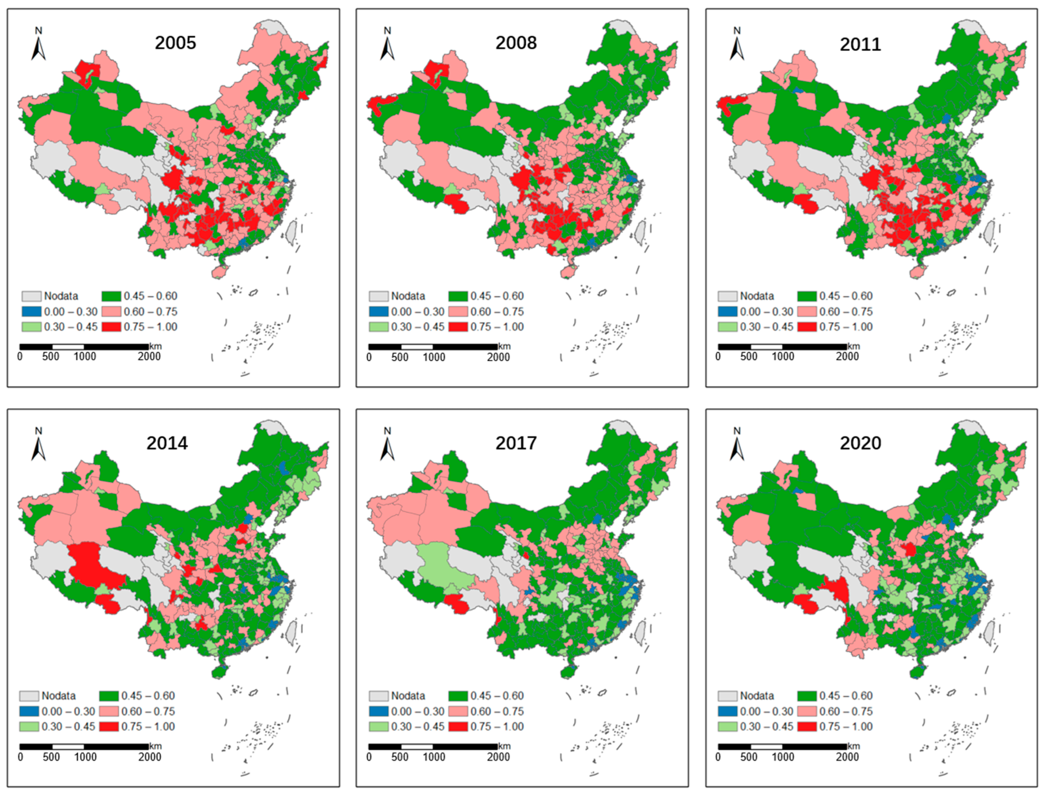
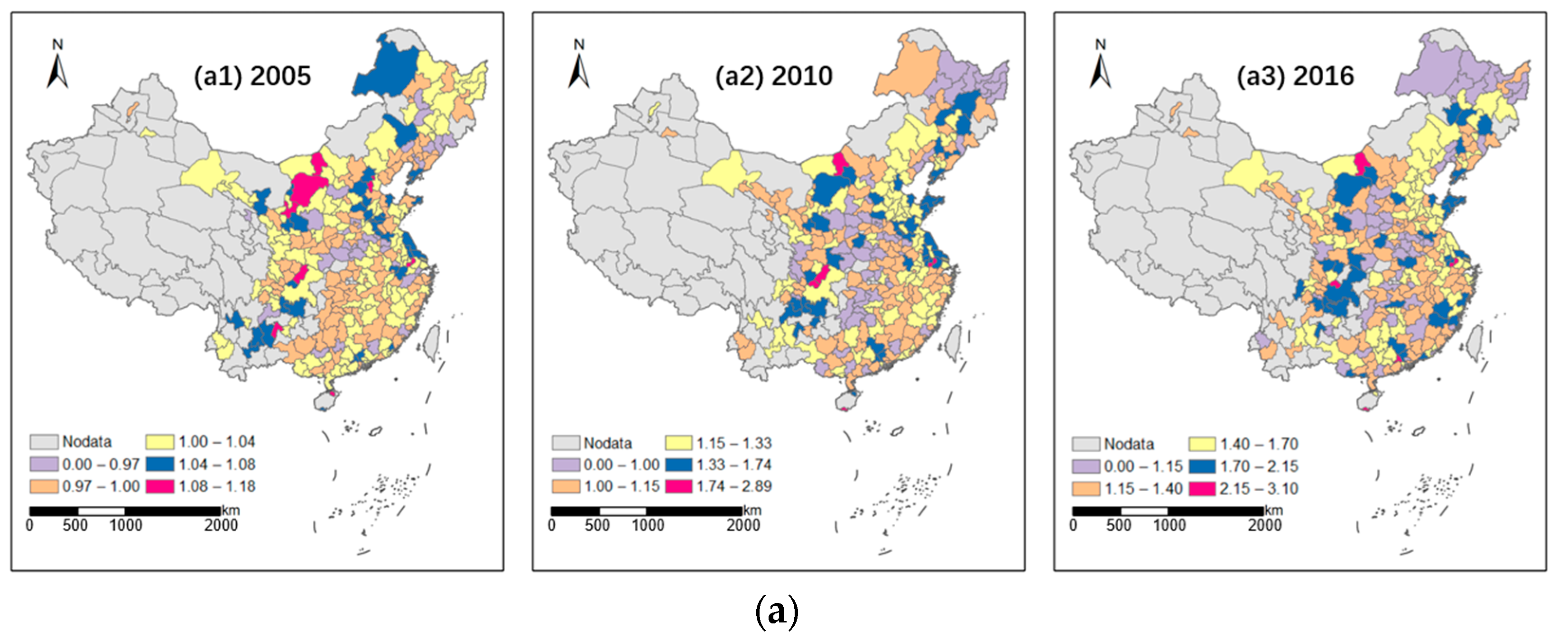
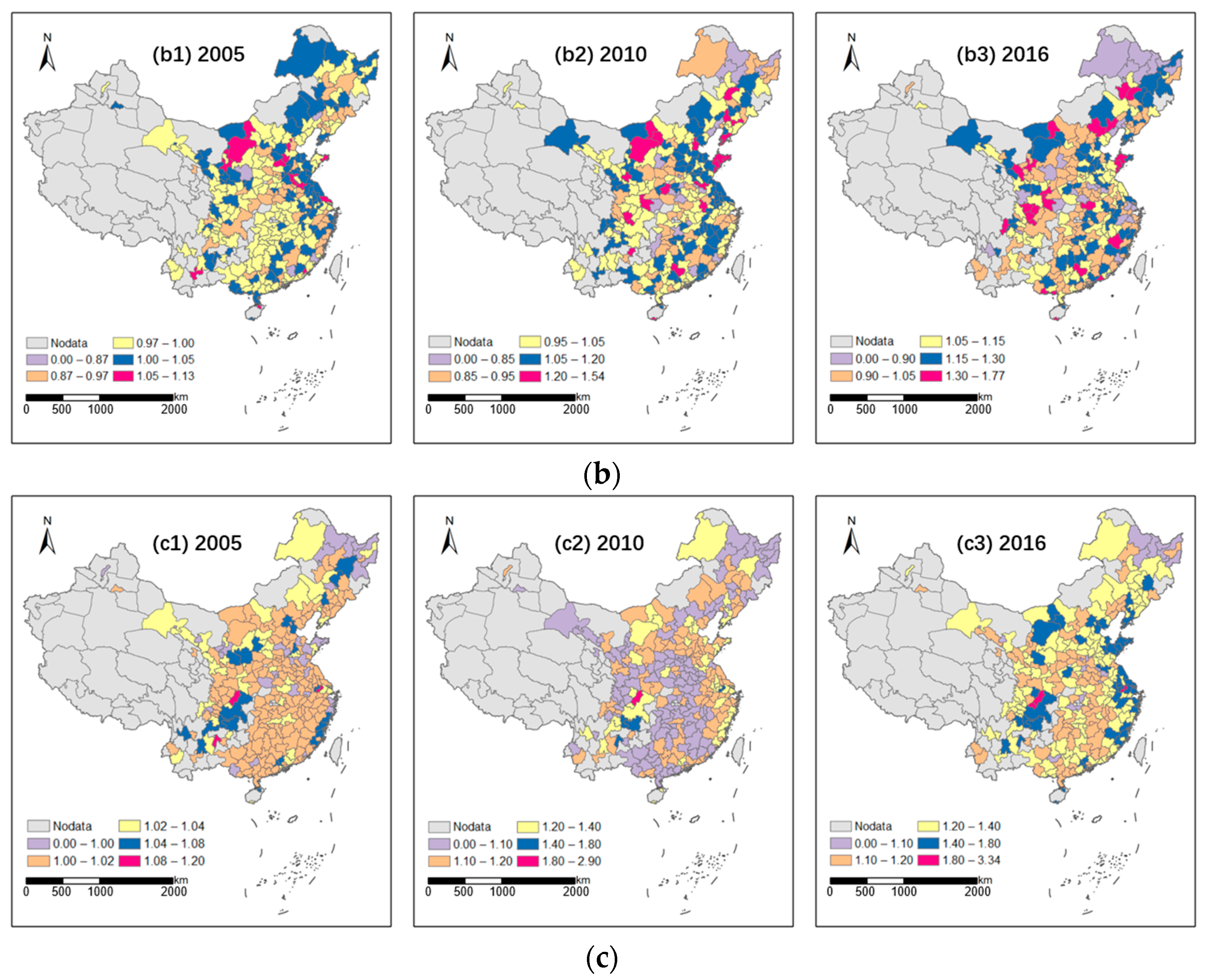
4.1. Urban Sprawl Index

Based on Equation (4), we calculated the urban sprawl index of 325 Chinese cities from 2005 to 2020, which are geo-visualized in Figure 1.

Overall, the urban sprawl index presented a decreasing trend from 2005 to 2020, indicating that urban expansion in China has remarkably slowed down. At the early stage of urbanization, namely in 2005, we observed that most cities, notably in central and southwestern China, for example, Yibin and Bazhou in Sichuan province, Tongren, and Qian’nan in Guizhou province, Chamdo and Shan’nan in Tibet, and Nujiang in Yunan, had high levels of urban sprawl, which indicated that they were accelerating urbanization. This is because The Western Development Strategy and the Rise of Central China policies were implemented at the beginning of the 21st century. In contrast, the most economically developed cities in the east, such as Beijing, Suzhou, and Shanghai, had the smallest sprawl index, indicating that they had the compact urban layout and had been urbanized. The implication here is that eastern cities had experienced rapid urban expansion that began with the reform and opening-up policy implemented in 1978. From 2005 to 2020, we notice that the area with a high urban sprawl index became narrow, indicating that the urbanization process of these cities had entered the post-urbanization era. We find that in 2020, very few cities had high indices, while the majority had ceased rapid urban expansion.

4.2. GTFP Scores

Based on Equation (1), the GTFP score of each Chinese city could be calculated; the scores were also geo-visualized in maps. For simplicity, the spatial distribution of GTFP scores in 2005, 2010, and 2016 are given in Figure 2a.

We observed that overall GTFP scores presented an increasing trend during the sample period, but nevertheless showed distinct spatial differences. Specifically, the high scores of the cities were mainly located in the east, while the western cities usually had lower GTFP scores. However, several cities, such as Ordos in Inner Mongolia, the cities in Shandong Peninsula, and the Yangtze River urban agglomeration, did have high GTFP scores. We also noticed that the low GTFP scores were primarily concentrated in the Hebei and Henan provinces in central China. Moreover, from 2010 to 2016, GTFP scores in the Northeastern cities had decreased. This signaled that these cities with low scores could not realize high-quality sustainable development. In other words, they are likely to face a huge challenge during the economic transition. In addition, the spatial distribution of the EC and TC in 2005, 2010, and 2016 are also given in Figure 2b,c. We observed that EC scores had a similar pattern as the GTFP in Figure 2a. Compared to GTFP and the EC, the TC scores of Chinese cities showed smaller variations in 2005. However, from 2010 to 2016, they had bigger changes in their spatial distributions, which indicated an increasing trend. The implication here is that technical change may be the fundamental contributor to GTFP.

Conversely, we found that the GTFP, TC, and EC scores of Chinese cities in maps were not randomly distributed, indicating spatial spillovers. Technically, we observed strong spatial dependence from Figure 2. Hence, the Moran’s I tests with three types of different spatial weights matrices were performed by Stata 17.0 software. The results are summarized in

Table 2. Results of Moran’s I test for GTFP, TC and EC scores of Chinese cities.

Moran’s I	Inverse			K3			Rook
	LnGTFP	LnTC	LnEC	LnGTFP	LnTC	LnEC	LnGTFP	LnTC	LnEC
2005	0.041 ***	0.018	0.029 *	0.181 ***	0.202 ***	0.135 ***	0.163 ***	0.009	0.105 **
	(2.532)	(1.249)	(1.826)	(4.24)	(4.858)	(3.19)	(3.589)	(0.276)	(2.347)
2006	0.070 ***	0.025 *	0.055 ***	0.262 ***	0.226 ***	0.204 ***	0.204 ***	0.064	0.155 ***
	(4.103)	(1.67)	(3.274)	(6.088)	(5.497)	(4.751)	(4.471)	(1.526)	(3.411)
2007	0.061 ***	0.020	0.036 **	0.240 ***	0.313 ***	0.172 ***	0.219 ***	0.086 **	0.170 ***
	(3.607)	(1.418)	(2.192)	(5.6)	(7.684)	(4.019)	(4.793)	(2.037)	(3.738)
2008	0.064 ***	0.028 *	0.050 ***	0.238 ***	0.261 ***	0.154 ***	0.205 ***	0.103 **	0.170 ***
	(3.808)	(1.909)	(3.018)	(5.547)	(6.518)	(3.607)	(4.497)	(2.467)	(3.736)
2009	0.061 ***	0.040 ***	0.041 **	0.243 ***	0.262 ***	0.158 ***	0.207 ***	0.136 ***	0.158 ***
	(3.645)	(2.617)	(2.51)	(5.664)	(6.538)	(3.704)	(4.532)	(3.229)	(3.474)
2010	0.065 ***	0.042 ***	0.049 ***	0.274 ***	0.272 ***	0.155 ***	0.193 ***	0.137 ***	0.125 ***
	(3.823)	(2.714)	(2.952)	(6.377)	(6.76)	(3.624)	(4.235)	(3.247)	(2.763)
2011	0.070 ***	0.042 ***	0.052 ***	0.309 ***	0.334 ***	0.165 ***	0.194 ***	0.132 ***	0.127 ***
	(4.099)	(2.666)	(3.125)	(7.179)	(8.104)	(3.865)	(4.254)	(3.047)	(2.813)
2012	0.078 ***	0.043 ***	0.056 ***	0.318 ***	0.360 ***	0.171 ***	0.187 ***	0.137 ***	0.114 **
	(4.548)	(2.682)	(3.333)	(7.393)	(8.648)	(4.003)	(4.099)	(3.131)	(2.529)
2013	0.064 ***	0.049 ***	0.053 ***	0.309 ***	0.402 ***	0.160 ***	0.142 ***	0.154 ***	0.077 **
	(3.754)	(3.023)	(3.152)	(7.171)	(9.517)	(3.734)	(3.127)	(3.462)	(1.74)
2014	0.062 ***	0.052 ***	0.051 ***	0.323 ***	0.388 ***	0.177 ***	0.161 ***	0.161 ***	0.099 ***
	(3.684)	(3.21)	(3.039)	(7.496)	(9.214)	(4.128)	(3.542)	(3.628)	(2.199)
2015	0.056 ***	0.055 ***	0.033 **	0.32 ***	0.421 ***	0.176 ***	0.163 ***	0.184 ***	0.072
	(3.314)	(3.312)	(2.026)	(7.424)	(9.91)	(4.101)	(3.583)	(4.102)	(1.62)
2016	0.050 ***	0.054 ***	0.020	0.308 ***	0.429 ***	0.204 ***	0.143 ***	0.178 ***	0.066
	(2.973)	(3.301)	(1.322)	(7.128)	(10.085)	(4.752)	(3.155)	(3.977)	(1.502)

Note: Z statistics in parentheses; *** p < 0.01, ** p < 0.05, and * p < 0.1.

.

On the one hand, Table 2 informs us that the annual Moran’s I value of the GTFP, TC and EC with Inverse, K3, and Rook spatial weights matrices were significant and positive, which implies that spatial spillovers were confirmed. On the other hand, it signals that the conclusions are robust and convincing when utilizing three matrices. Hence, spatial spillovers should be incorporated in the models when investigating the impacts of urban sprawl on the GTFP, TC, and EC.

5. Empirical Results

5.1. Classical Models

We first focused on the non-spatial econometric models, as they are usually treated as benchmark models. Estimation results are presented in

Table 3. Results of non-spatial panel data models (Key variable: US = sprawl level).

Variable	Model (1)	Model (2)	Model (3)	Model (4)	Model (5)	Model (6)
	LnGTFP	LnTC	LnEC	LnGTFP	LnTC	LnEC
LnUS	−0.073 ***	−0.049 ***	−0.024 ***	−0.050 ***	−0.034 ***	−0.015 *
	(0.000)	(0.000)	(0.007)	(0.000)	(0.000)	(0.061)
LnFDI	−0.001	0.004 **	−0.006 **	0.001	0.004 **	−0.002
	(0.681)	(0.013)	(0.016)	(0.697)	(0.019)	(0.339)
LnEdu	0.143 ***	0.078 ***	0.065 ***	0.129 ***	0.074 ***	0.054 ***
	(0.000)	(0.000)	(0.000)	(0.000)	(0.000)	(0.000)
LnStructure	0.180 ***	0.130 ***	0.050 ***	0.153 ***	0.109 ***	0.044 ***
	(0.000)	(0.000)	(0.000)	(0.000)	(0.000)	(0.000)
LnFD	−0.066 ***	−0.030 ***	−0.035 ***	−0.023 **	−0.007	−0.015 **
	(0.000)	(0.000)	(0.000)	(0.018)	(0.237)	(0.036)
LnInnov	−0.006 **	0.003 *	−0.009 ***	−0.008 ***	0.002	−0.010 ***
	(0.048)	(0.057)	(0.000)	(0.005)	(0.345)	(0.000)
Fixed effects	Yes	Yes	Yes	No	No	No
R2	0.563	0.646	0.200	−	−	−
Obs.	3324	3324	3324	3324	3324	3324

Note: Standard errors in parentheses; *** p < 0.01, ** p < 0.05, and * p < 0.1.

.

As shown in Table 3, the estimation results of the fixed effects models (Model (1), Model (2), and Model (3)) are given. For completeness and robustness, we also estimated the random effects models (Model (4), Model (5), and Model (6)). To judge which one was more suitable, a Hausman test was conducted, and the results were in favor of the fixed effects models.

From Model (1), we observed that the coefficient of US was significant and negative, indicating that urban sprawl hindered GTFP. We noticed that Edu and Structure had significant impacts on GTFP, while FD and Innov showed negative impacts. However, FDI was statistically insignificant. In addition, by regarding Models (2) and (3) in a similar vein, we noted that the variable US had a negative impact on TC and EC, indicating that urban sprawl also reduced TC and EC. We noticed that FDI had a positive impact on TC and a negative impact on EC. Edu and Structure were positively correlated with TC and EC, while FD was negatively correlated with TC and EC. Finally, Innov showed a positive impact on TC, but a negative impact on EC.

From the above analysis, we noticed that, except for the US variable, other variables had different impacts on the GTFP, TC, and EC. One of the main explanations for this finding is that the non-spatial fixed effects models ignore spatial spillovers, and biased estimates may be obtained. To cope with this issue, we adopted the fixed effects spatial lag panel data models.

5.2. Spatial Lag Panel Data Models

Based on Equation (7), we treated the GTFP, TC, and EC as dependent variables, and used Stata 17.0 software to apply the maximum likelihood estimation method to obtain the results of the two-way fixed effects spatial lag panel data models; we applied three spatial weights matrices. The results are summarized in

Table 4. Results of two-way fixed effects spatial lag panel data models (Key variable: US = sprawl level).

Matrix	Inverse			K3			Rook
Model	Model (7)	Model (8)	Model (9)	Model (10)	Model (11)	Model (12)	Model (13)	Model (14)	Model (15)
Variable	LnGTFP	LnTC	LnEC	LnGTFP	LnTC	LnEC	LnGTFP	LnTC	LnEC
LnUS	−0.031 ***	−0.035 ***	0.004	−0.020 *	−0.024 ***	0.005	−0.031 ***	−0.034 ***	0.003
	(0.008)	(0.000)	(0.652)	(0.064)	(0.000)	(0.601)	(0.008)	(0.000)	(0.717)
LnFDI	−0.010 ***	−0.008 ***	−0.002	−0.009 ***	−0.006 ***	−0.002	−0.010 ***	−0.007 ***	−0.003
	(0.001)	(0.000)	(0.371)	(0.003)	(0.000)	(0.323)	(0.002)	(0.000)	(0.315)
LnEdu	0.044 ***	−0.000	0.044 ***	0.041 ***	−0.000	0.045 ***	0.045 ***	−0.002	0.047 ***
	(0.000)	(0.998)	(0.000)	(0.000)	(0.976)	(0.000)	(0.000)	(0.767)	(0.000)
LnStructure	0.058 ***	0.049 ***	0.009	0.041 ***	0.028 ***	0.005	0.050 ***	0.045 ***	0.003
	(0.000)	(0.000)	(0.407)	(0.003)	(0.000)	(0.620)	(0.000)	(0.000)	(0.772)
LnFD	−0.098 ***	−0.061 ***	−0.036 ***	−0.089 ***	−0.050 ***	−0.037 ***	−0.100 ***	−0.061 ***	−0.038 ***
	(0.000)	(0.000)	(0.000)	(0.000)	(0.000)	(0.000)	(0.000)	(0.000)	(0.000)
LnInnov	0.015 ***	0.010 ***	0.004 *	0.014 ***	0.009 ***	0.004	0.015 ***	0.011 ***	0.004
	(0.000)	(0.000)	(0.098)	(0.000)	(0.000)	(0.112)	(0.000)	(0.000)	(0.110)
ρ	0.322 ***	0.356 ***	0.320 ***	0.296 ***	0.410 ***	0.174 ***	0.121 ***	0.110 ***	0.190 ***
	(0.000)	(0.000)	(0.000)	(0.000)	(0.000)	(0.000)	(0.000)	(0.000)	(0.000)
R2	0.133	0.004	0.048	0.130	0.011	0.039	0.105	0.012	0.032
Log−Likelihood	3935.155	6005.987	4764.773	4012.763	6211.783	4772.284	3928.726	4753.573	6021.162
Obs.	3324	3324	3324	3324	3324	3324	3324	3324	3324

Note: Standard errors in parentheses; *** p < 0.01, ** p < 0.05, and * p < 0.1.

.

In the case of GTFP, the results of the three models with Inverse, K3 and Rook spatial weights matrices (e.g., Models (7), (10), and (13)) are given. We observed that all variables of the three models were statistically significant, implying that these three models were all well fitted. The log-likelihood statistic could help us determine which one was the best fitted. Based on the criterion that the higher the log-likelihood statistic, the better fitted, we noticed that Model (10) with K3 matrix had the highest log-likelihood statistic (4012.763), which is regarded as the best one. We also considered K4, K5, and K6 matrices to repeat the spatial lag panel data models and found that it remained as the best fitted.

From Model (10), we noted that the spatial autoregressive coefficient $\rho$ (0.130) was significant and positive, indicating the existence of spatial spillovers of the GTFP of Chinese cities in line with the conclusions of Moran’s I test. It also implied that increases in GTFP scores of neighboring cities promoted the improvements of GTFP in a nearby city. In other words, the spatial dependence of GTFP can be explicitly incorporated in the model, and thus the spatial lag panel data model was better fitted than the non-spatial panel data model.

When we considered the US variable, we found that it was still significant and negative, and conformed to that of Model (1). However, we observed that the estimated coefficient (−0.020) of Model (10) was smaller (in absolute value) than that (−0.073) of Model (1). The implication here is that the upward estimate could be obtained if the spatial spillovers of GTFP were omitted from the regression models. The negative coefficient shows that over-urban expansion leads to GTFP losses, because urban sprawl makes the city low-density and thus weakens agglomeration externalities, e.g., resource allocation and sharing, highly efficient resource matching, and knowledge spillovers. In contrast, large-scale urbanization stimulates widespread resource consumption, such as fossil energy, which leads to pollutant emissions, worsening damage to the environment, and damage to prior GTFP gains. In sum, accelerated urban expansion during the past decades has now become a hindrance to further GTFP improvements in China.

The FDI variable was found to have a significant and negative effect on GTFP, indicating that FDI could reduce GTFP. One possible explanation for this finding is that considerable FDI inflows may exert a pollution haven effect. Since China has had lower environmental standards in past years, pollution-intensive industries have tended to migrate from developed countries to China, leading not only to increased local employment and income levels, but also to environmental degradation caused by industrial pollutants. Hence, environmental degradation and consequent GTFP losses could be partly explained by the pollution haven effect.

The Edu variable exerted a significant and positive impact on GTFP, indicating that an increase in expenditure on education contributed to improving GTFP, and this was in line with the conclusion of a study by Xiao and You [61]. It also implied that education spending plays an important role in the GTFP improvements. In recent years, central government and local governments have increased expenditure on education in a bid to enhance human capital, which has been beneficial to technical progress and GTFP gains.

Similarly, the Structure variable was found to be positively correlated with GTFP, indicating that the higher the ratio of the tertiary industry, the better the GTFP. Ever since the reform and opening-up policy began, China has accelerated industrialization and improved the life standards of Chinese people. However, large-scale industrialization has also revealed the opposite side of the coin by introducing numerous industrial pollutants, thus worsening the environment and lowering GTFP. In the past ten years, however, Chinese policy makers have understood the pollution consequences and begun to implement a series of policies to optimize the industrial structure; they have done so by increasing the share of the tertiary industry, since it is characterized by high value-added and low pollutant emissions. Correspondingly, the tertiary industry accounted for more than 50% of GDP in 2020, which is beneficial for GTFP improvements.

We found that the FD variable had a significant and negative impact on GTFP, and this was in line with the study of Song et al. [18]. The implication here is that fiscal decentralization does not improve GTFP. One possible explanation is that local governments tend to compete for economic performance at the expense of environmental construction and improvement.

Lastly, regarding the estimated coefficient of the Inno variable, results showed that it was significant and positive, indicating that technological progress proxied by R&D expenditure contributes to GTFP improvements. This variable has been identified as the foremost contributor to productivity gains without worsening the environment or undermining economic growth. In other words, an increase in R&D expenditure makes it possible to improve production efficiency and to effectively mitigate pollutant emissions and discharges during the industrial production processes [62]. Hence, municipalities should enlarge the expenditure on R&D to encourage technological progress and improve GTFP.

In the case of the TC and EC, Models (11) and (12) had similar findings with Model (10). In particular, we focused on the impact of US on the TC and EC. Results showed that it had a significant and negative impact on the TC, but an insignificant impact on the EC, though negative. From the above analysis, we reached two conclusions. One is that urban sprawl does not impact efficiency change, but rather impairs technical efficiency. The other is an interesting finding: that urban sprawl could first reduce technical efficiency, and then hinder GTFP improvements.

6. Conclusions and Discussion

In the process of urbanization during the 21st century, special attention must be paid to the optimization of urban spatial layouts and GTFP improvements. Therefore, to investigate the impact of urban sprawl on GTFP in China, this research first used DMSP/OLS and NPP/VIIRS nighttime lighting data to calculate the urban sprawl indicator, and then analyzed the spatio-temporal variations. Next, we adopted the global Malmquist–Luenberger index to compute the GTFP scores of Chinese cities from 2005 to 2016. Lastly, we incorporated spatial spillovers of GTFP and built the spatial lag panel data models to examine the impact of urban sprawl on the GTFP, TC, and EC. The main findings of this research are as follows.

In general, from the temporal dimension, the growth rate of urban sprawl has slowed down in recent years. From the spatial dimension, we observed significant differences in the levels of urban sprawl of Chinese cities in space. Notably, the east has urbanized, while the cities in central and southwestern China increased their urban expansion from 2005 to 2011. From the spatio-temporal variations of the GTFP of Chinese cities, we found that average GTFP scores fluctuated during the sample period. From 2013 onwards, they started to increase. Furthermore, higher GTFP scores were mainly concentrated in the economically developed eastern region and in the environmentally friendly southwestern region. The estimation results of the two-way fixed effects spatial lag panel data models revealed that urban sprawl had a negative impact on the TC and GTFP, indicating that rapid urban expansion was not conducive to improving GTFP. We also found that the expansion of urban land area was a contributor to lowering GTFP, while population growth and agglomeration did not exert an impact on GTFP.

From the findings of this research, a series of policy implications can be suggested to promote a new type of urbanization characterized by optimizing the spatial layout and realizing high-quality development. First, generally, urban sprawl in China symbolizes the rapid and low-density expansion of urban space, which has led to a series of problems, e.g., high transaction costs, traffic congestion, restricted knowledge spillovers, and low productivity. To cope with the consequences, municipal governments could limit the level of urban sprawl and build compact cities from a perspective of stable, long-term, and sustainable urban development. In the early stages of urban agglomeration and expansion, moderate urban sprawl can promote the rapid flow of resources and allocations within the city, accelerate the formation of urban agglomeration, and provide enough space for industrial transfer and industrial upgrading in the sprawling suburban areas due to low land costs, which effectively contribute to GTFP improvement in various ways.

Second, since the impact of urban sprawl on GTFP is negative in the urbanization process, rapid urban expansion should be tightly controlled. Otherwise, the over-expansion of urban areas is likely to lead to productivity and social efficiency losses. When facing increased population density in city centers, municipal governments should not relieve the pressure on population agglomeration through unlimited urban land expansion, but instead should take productivity-oriented measures and actions to scientifically delineate urban boundaries and strengthen the accommodation and the population absorption of cities. This can be achieved by optimizing the layout of urban infrastructure to improve the efficiency of public services and reduce negative externalities, without undermining the improvements of urban productivity and efficiency. On the other hand, for megacities with a large urban area, the priority could be to reshape a more reasonable urban spatial structure and develop widespread public transportation to enhance the carrying capacity of megacities without over expanding urban space.

Third, the urban sprawl level varies from city to city in China. Specifically, eastern cities have already been urbanized, so the overall urban sprawl in the east has already slowed. However, for the middle and western cities, we should be more aware of the intensification of urban sprawl, since they are continuing to accelerated urbanization. It is possible to forecast that urban sprawl will become a hindrance to GTFP improvement. Hence, municipal governments should adopt city-specific urban planning and discreetly implement urban sprawl policies to better encourage a compact and intensive urban development approach.

Fourth, the urban area should strive to match a reasonable population size and industrial agglomeration so that high-quality urban economic growth with high productivity can be realized. For instance, a number of new industrial parks in the suburban areas should be strictly controlled, which means that new urban construction land should be reasonably developed; local governments should consider city-specific conditions, including population size, industrial structure, and even urban geography, to promote population agglomeration and adopt appropriate industry optimization policies towards the sustainable development of Chinese cities.

There are some limitations in this research that can, however, be resolved in future work. Due to data unavailability while evaluating the GTFP scores of Chinese cities, we could not update the dataset up to 2020. Future work should extend the dataset or seek alternative indicators to replace the unavailable data, and then re-quantify the impact of urban sprawl. There may also be a problem of reverse causality between urban sprawl and productivity. However, due to the lack of corresponding tests in the spatial econometric model specification, we were unable to perform the tests in this work. Future research should consider endogeneity and reverse causality issues and re-examine the nexus between urban sprawl and productivity in China.

References

1. Yu, H.; Liu, Y.; Zhao, J.; Li, G. Urban Total Factor Productivity: Does Urban Spatial Structure Matter in China? Sustainability 2019, 12, 214. [Google Scholar] [CrossRef] [Green Version]
2. World Bank. Urban China: Toward Efficient, Inclusive, and Sustainable Urbanization; World Bank: Washington, DC, USA, 2014. [Google Scholar]
3. National Bureau of Statistics of China. China Statistical Yearbook 2021; China Statistics Press: Beijing, China, 2021.
4. Deng, Y.; Qi, W.; Fu, B.; Wang, K. Geographical transformations of urban sprawl: Exploring the spatial heterogeneity across cities in China 1992–2015. Cities 2020, 105, 102415. [Google Scholar] [CrossRef]
5. Ministry of Housing and Urban-Rural Development of China. China Urban Construction Statistical Yearbook; China Statistics Press: Beijing, China, 2021.
6. Guan, X.; Wei, H.; Lu, S.; Dai, Q.; Su, H. Assessment on the urbanization strategy in China: Achievements, challenges and reflections. Habitat Int. 2018, 71, 97–109. [Google Scholar] [CrossRef]
7. Shi, K.; Xu, T.; Li, Y.; Chen, Z.; Gong, W.; Wu, J.; Yu, B. Effects of urban forms on CO2 emissions in China from a multi-perspective analysis. J. Environ. Manag. 2020, 262, 110300. [Google Scholar] [CrossRef]
8. Wei, Y.; Liu, H.; Song, W.; Yu, B.; Xiu, C. Normalization of time series DMSP-OLS nighttime light images for urban growth analysis with Pseudo Invariant Features. Landsc. Urban Plan. 2014, 128, 1–13. [Google Scholar] [CrossRef]
9. Guo, A.; Yang, J.; Xiao, X.; Xia, J.; Jin, C.; Li, X. Influences of urban spatial form on urban heat island effects at the community level in China. Sustain. Cities Soc. 2020, 53, 101972. [Google Scholar] [CrossRef]
10. Shao, S.; Li, X.; Cao, J. Urbanization promotion and haze pollution governance in China. Econ. Res. J. 2019, 2, 148–165. [Google Scholar]
11. Khan, S.A.R.; Zaman, K.; Zhang, Y. The relationship between energy-resource depletion, climate change, health resources and the environmental Kuznets curve: Evidence from the panel of selected developed countries. Renew. Sustain. Energy Rev. 2016, 62, 468–477. [Google Scholar] [CrossRef]
12. Mitchell, L.E.; Lin, J.C.; Bowling, D.R.; Pataki, D.E.; Strong, C.; Schauer, A.J.; Bares, R.; Bush, S.E.; Stephens, B.B.; Mendoza, D.; et al. Long-term urban carbon dioxide observations reveal spatial and temporal dynamics related to urban characteristics and growth. Proc. Natl. Acad. Sci. USA 2018, 115, 2912–2917. [Google Scholar] [CrossRef] [Green Version]
13. Mekonnen, M.M.; Hoekstra, A.Y. Global Anthropogenic Phosphorus Loads to Freshwater and Associated Grey Water Footprints and Water Pollution Levels: A High-Resolution Global Study. Water Resour. Res. 2018, 54, 345–358. [Google Scholar] [CrossRef] [Green Version]
14. Cheng, K.; Gao, D.; Zhuang, Y. The Mechanism and Effects of Urban Sprawl on Total Factor Productivity in Prefecture Level Cities of China: Based on DMSP/OLS and NPP/VIIRS Night Light Data. China Land Sci. 2021, 35, 90–100. (In Chinese) [Google Scholar]
15. Chen, D.; Lu, X.; Liu, X.; Wang, X. Measurement of the eco-environmental effects of urban sprawl: Theoretical mechanism and spatiotemporal differentiation. Ecol. Indic. 2019, 105, 6–15. [Google Scholar] [CrossRef]
16. Han, J. Can urban sprawl be the cause of environmental deterioration? Based on the provincial panel data in China. Environ. Res. 2020, 189, 109954. [Google Scholar] [CrossRef]
17. Shao, H.; Xia, H. The impact of urban sprawl on green total factor productivity in China. Resour. Sci. 2020, 42, 790. [Google Scholar] [CrossRef]
18. Song, M.; Du, J.; Tan, K.H. Impact of fiscal decentralization on green total factor productivity. Int. J. Prod. Econ. 2018, 205, 359–367. [Google Scholar] [CrossRef]
19. Xia, F.; Xu, J. Green total factor productivity: A re-examination of quality of growth for provinces in China. China Econ. Rev. 2020, 62, 101454. [Google Scholar] [CrossRef]
20. Wang, J.; Qu, S.; Peng, K.; Feng, Y. Quantifying urban sprawl and its driving forces in China. Discret. Dyn. Nat. Soc. 2019, 2019, 2606950. [Google Scholar] [CrossRef]
21. Fulton, W.B.; Pendall, R.; Nguyen, M.; Harrison, A. Who Sprawls Most?: How Growth Patterns Differ across the US; Brookings Institution, Center on Urban and Metropolitan Policy: Washington, DC, USA, 2001. [Google Scholar]
22. Kolankiewicz, L.; Beck, R. Weighing Sprawl Factors in Large US Cities. Available online: https://www.numbersusa.com/content/files/pdf/LargeCity%20Sprawl.pdf (accessed on 19 March 2001).
23. Galster, G.; Hanson, R.; Ratcliffe, M.R.; Wolman, H.; Coleman, S.; Freihage, J. Wrestling Sprawl to the Ground: Defining and measuring an elusive concept. Hous. Policy Debate 2001, 12, 681–717. [Google Scholar] [CrossRef]
24. Frenkel, A.; Ashkenazi, M. The integrated sprawl index: Measuring the urban landscape in Israel. Ann. Reg. Sci. 2008, 42, 99–121. [Google Scholar] [CrossRef]
25. Ewing, R.; Pendall, R.; Chen, D. Measuring Sprawl and Its Transportation Impacts. Transp. Res. Rec. 2003, 1831, 175–183. [Google Scholar] [CrossRef]
26. Sutton, P.C. A scale-adjusted measure of “Urban sprawl” using nighttime satellite imagery. Remote Sens. Environ. 2003, 86, 353–369. [Google Scholar] [CrossRef]
27. Qin, M.; Liu, X.; Tong, Y. Does urban sprawl exacerbate haze pollution–An empirical study of fine particles (PM2.5) in Chinese cities. Financ. Trade Econ. 2016, 37, 146–160. (In Chinese) [Google Scholar]
28. Sudhira, H.S.; Ramachandra, T.V.; Jagadish, K.S. Urban sprawl: Metrics, dynamics and modelling using GIS. Int. J. Appl. Earth Obs. Geoinf. 2004, 5, 29–39. [Google Scholar] [CrossRef]
29. Jat, M.K.; Garg, P.K.; Khare, D. Monitoring and modelling of urban sprawl using remote sensing and GIS techniques. Int. J. Appl. Earth Obs. Geoinf. 2008, 10, 26–43. [Google Scholar] [CrossRef]
30. Gao, B.; Huang, Q.; He, C.; Sun, Z.; Zhang, D. How does sprawl differ across cities in China? A multi-scale investigation using nighttime light and census data. Landsc. Urban Plan. 2016, 148, 89–98. [Google Scholar] [CrossRef]
31. Guan, D.; He, X.; He, C.; Cheng, L.; Qu, S. Does the urban sprawl matter in Yangtze River Economic Belt, China? An integrated analysis with urban sprawl index and one scenario analysis model. Cities 2020, 99, 102611. [Google Scholar] [CrossRef]
32. Feng, Z.; Peng, J.; Wu, J. Using DMSP/OLS nighttime light data and K–means method to identify urban–rural fringe of megacities. Habitat Int. 2020, 103, 102227. [Google Scholar] [CrossRef]
33. Chen, D.; Lu, X.; Hu, W.; Zhang, C.; Lin, Y. How urban sprawl influences eco-environmental quality: Empirical research in China by using the Spatial Durbin model. Ecol. Indic. 2021, 131, 108113. [Google Scholar] [CrossRef]
34. Wu, Y.; Li, C.; Shi, K.; Liu, S.; Chang, Z. Exploring the effect of urban sprawl on carbon dioxide emissions: An urban sprawl model analysis from remotely sensed nighttime light data. Environ. Impact Assess. Rev. 2022, 93, 106731. [Google Scholar] [CrossRef]
35. Shao, Z.; Sumari, N.S.; Portnov, A.; Ujoh, F.; Musakwa, W.; Mandela, P.J. Urban sprawl and its impact on sustainable urban development: A combination of remote sensing and social media data. Geo-Spat. Inf. Sci. 2021, 24, 241–255. [Google Scholar] [CrossRef]
36. Lu, C.; Li, L.; Lei, Y.; Ren, C.; Su, Y.; Huang, Y.; Chen, Y.; Lei, S.; Fu, W. Coupling Coordination Relationship between Urban Sprawl and Urbanization Quality in the West Taiwan Strait Urban Agglomeration, China: Observation and Analysis from DMSP/OLS Nighttime Light Imagery and Panel Data. Remote Sens. 2020, 12, 3217. [Google Scholar] [CrossRef]
37. Wang, L.; Li, W.; Wang, P.; Liu, X.; Yang, F.; Qu, J.J. Spatiotemporal characterization of the urban sprawl and its impacts on urban island in China with DMSP/OLS and MODIS measurements. Theor. Appl. Climatol. 2019, 138, 293–303. [Google Scholar] [CrossRef]
38. Zhang, D.; Zhou, C.; He, B. Spatial and temporal heterogeneity of urban land area and PM2.5 concentration in China. Urban Clim. 2022, 45, 101268. [Google Scholar] [CrossRef]
39. Zhao, X.; Shang, Y.; Song, M. What kind of cities are more conducive to haze reduction: Agglomeration or expansion? Habitat Int. 2019, 91, 102027. [Google Scholar] [CrossRef]
40. Yang, Y.; Yan, D. Does urban sprawl exacerbate urban haze pollution? Environ. Sci. Pollut. Res. 2021, 28, 56522–56534. [Google Scholar] [CrossRef] [PubMed]
41. Zhang, H. The Impact of Urban Sprawl on Environmental Pollution: Empirical Analysis from Large and Medium-Sized Cities of China. Int. J. Environ. Res. Public Health 2021, 18, 8650. [Google Scholar] [CrossRef]
42. Feng, Y.; Wang, X. Effects of urban sprawl on haze pollution in China based on dynamic spatial Durbin model during 2003–2016. J. Clean. Prod. 2020, 242, 118368. [Google Scholar] [CrossRef]
43. Yang, X.; Wang, J.; Cao, J.; Ren, S.; Ran, Q.; Wu, H. The spatial spillover effect of urban sprawl and fiscal decentralization on air pollution: Evidence from 269 cities in China. Empir. Econ. 2022, 63, 847–875. [Google Scholar] [CrossRef]
44. Shi, X.; Matsui, T.; Machimura, T.; Haga, C.; Hu, A.; Gan, X. Impact of urbanization on the food–water–land–ecosystem nexus: A study of Shenzhen, China. Sci. Total Environ. 2022, 808, 152138. [Google Scholar] [CrossRef]
45. Tao, A.; Liang, Q.; Kuai, P.; Ding, T. The Influence of Urban Sprawl on Air Pollution and the Mediating Effect of Vehicle Ownership. Processes 2021, 9, 1261. [Google Scholar] [CrossRef]
46. Cheng, Z.; Hu, X. The effects of urbanization and urban sprawl on CO2 emissions in China. Environ. Dev. Sustain. 2022, 1–17. [Google Scholar] [CrossRef]
47. Schwaab, J.; Deb, K.; Goodman, E.; Lautenbach, S.; van Strien, M.; Grêt-Regamey, A. Reducing the loss of agricultural productivity due to compact urban development in municipalities of Switzerland. Comput. Environ. Urban Syst. 2017, 65, 162–177. [Google Scholar] [CrossRef]
48. Fallah, B.N.; Partridge, M.D.; Olfert, M.R. Urban sprawl and productivity: Evidence from US metropolitan areas. Pap. Reg. Sci. 2011, 90, 451–472. [Google Scholar] [CrossRef]
49. Park, J.-I.; Kim, J.-O. Does industrial land sprawl matter in land productivity? A case study of industrial parks of South Korea. J. Clean. Prod. 2022, 334, 130209. [Google Scholar] [CrossRef]
50. Monkkonen, P.; Montejano, J.; Guerra, E.; Caudillo, C. Compact cities and economic productivity in Mexico. Urban Stud. 2020, 57, 2080–2097. [Google Scholar] [CrossRef]
51. Zhang, Y.; Wang, L.; Tang, Z.; Zhang, K.; Wang, T. Spatial effects of urban expansion on air pollution and eco-efficiency: Evidence from multisource remote sensing and statistical data in China. J. Clean. Prod. 2022, 367, 132973. [Google Scholar] [CrossRef]
52. Yao, Y.; Pan, H.; Cui, X.; Wang, Z. Do compact cities have higher efficiencies of agglomeration economies? A dynamic panel model with compactness indicators. Land Use Policy 2022, 115, 106005. [Google Scholar] [CrossRef]
53. Lu, X.; Chen, D.; Wang, Y. Is Urban Sprawl Decoupled from the Quality of Economic Growth? Evidence from Chinese Cities. Sustainability 2020, 12, 218. [Google Scholar] [CrossRef] [Green Version]
54. Pastor, J.T.; Lovell, C.A.K. A global Malmquist productivity index. Econ. Lett. 2005, 88, 266–271. [Google Scholar] [CrossRef]
55. Oh, D.-H. A global Malmquist-Luenberger productivity index. J. Product. Anal. 2010, 34, 183–197. [Google Scholar] [CrossRef]
56. Wu, Y.; Shi, K.; Chen, Z.; Liu, S.; Chang, Z. Developing Improved Time-Series DMSP-OLS-Like Data (1992–2019) in China by Integrating DMSP-OLS and SNPP-VIIRS. IEEE Trans. Geosci. Remote Sens. 2021, 60, 1–14. [Google Scholar] [CrossRef]
57. Cui, Y.; Shi, K.; Jiang, L.; Qiu, L.; Wu, S. Identifying and evaluating the nighttime economy in China using multisource data. IEEE Geosci. Remote Sens. Lett. 2020, 18, 1906–1910. [Google Scholar] [CrossRef]
58. Doll, C.H.; Muller, J.-P.; Elvidge, C.D. Night-time Imagery as a Tool for Global Mapping of Socioeconomic Parameters and Greenhouse Gas Emissions. AMBIO A J. Hum. Environ. 2000, 29, 157–162. [Google Scholar] [CrossRef]
59. Moran, P.A. Notes on continuous stochastic phenomena. Biometrika 1950, 37, 17–23. [Google Scholar] [CrossRef]
60. Elhorst, J.P. Spatial Econometrics from Cross-Sectional Data to Spatial Panels; Springer: Berlin/Heidelberg, Germany, 2014. [Google Scholar]
61. Xiao, H.; You, J. The Heterogeneous Impacts of Human Capital on Green Total Factor Productivity: Regional Diversity Perspective. Front. Environ. Sci. 2021, 9, 713562. [Google Scholar] [CrossRef]
62. Jiang, L.; He, S.; Zhou, H.; Kong, H.; Wang, J.; Cui, Y.; Wang, L. Coordination between sulfur dioxide pollution control and rapid economic growth in China: Evidence from satellite observations and spatial econometric models. Struct. Chang. Econ. Dyn. 2021, 57, 279–291. [Google Scholar] [CrossRef]
Figure 1. Spatial distribution of urban sprawl index of Chinese cities from 2005 to 2020.
Land 11 02120 g001
Figure 2. (a). Spatial distribution of GTFP scores of Chinese cities in 2005, 2010, and 2016. (b). Spatial distribution of EC scores of Chinese cities in 2005, 2010, and 2016. (c). Spatial distribution of TC scores of Chinese cities in 2005, 2010, and 2016.
Land 11 02120 g002aLand 11 02120 g002b