Article

Spatial Pattern and Ecological Process Difference Analyses of the Boundary Habitats of a Treeline Patch: A Case Study from the Li Mountain, North China

1
School of Water Resources and Environmental Engineering, East China University of Technology, Nanchang 330013, China
2
Key Laboratory of Biodiversity Sciences and Ecological Engineering, Ministry of Education, College of Life Sciences, Beijing Normal University, Beijing 100875, China
3
School of Metallurgy and Environment, Central South University, Changsha 410083, China
4
Department of Biological Sciences, University of Veterinary and Animal Sciences, Lahore 54000, Pakistan
*
Author to whom correspondence should be addressed.
Land 2022, 11(11), 2064; https://doi.org/10.3390/land11112064
Submission received: 23 October 2022 / Revised: 11 November 2022 / Accepted: 13 November 2022 / Published: 17 November 2022
(This article belongs to the Section Land Systems and Global Change)

Abstract

:
Treeline patches are among Earth’s most sensitive and are important model ecosystems for assessing climate change trends. To explore ecological factors that limit the species’ survival in treelines, the treeline patch of Li Mountain National Nature Reserve was selected as the research site. Pinus armandii (P. armandii), Betula albo-sinensis (B. albo-sinensis), and Betula utilis (B. utilis) were selected as research species based on their dominance. Two 50 m × 50 m plots were established separately from the upper and lower limits of the highest treeline patch for point pattern analysis. Five 10 m × 10 m quadrats per plot were sampled to investigate the flora and environmental factors. The results showed that: (1) Slope and community composition at tree layer in quadrates had significant differences between upper and lower limits. Pinus armandii had a greater population size at the upper limit. Seedling recruitment restricted population development for B. albo-sinensis at the lower limit and B. utilis at the upper limit and less regeneration of B. albo-sinensis at the upper limit. (2) More aggregation scales occurred at the upper limit, and P. armandii had more aggregation scales than the other two species at 0–25 m. The heterogeneity caused by density distribution affected P. armandii pattern at the upper limit, and heterogeneity of seed dispersal could explain species patterns in both limits. Distinctness of size difference may have an influence on inter-specific species correlations.

1. Introduction

Since the last century, global warming has been a significant problem, especially regarding vegetation composition and spatial distribution of an ecosystem in a high-altitude region [1,2]. Alpine treeline dynamics have proved important for predicting climate change patterns and for studying species response strategies [3]. The term “treeline” is typically defined as a transition zone extending from the uppermost part of a closed canopy forest to the scattered individuals [4]. The treeline patch extends from the lowermost of <50% coverage forest to an open meadow [5]. Climate research on high-elevation treelines has investigated environmental factors, such as high sunlight [6,7], low temperature [8,9], topography [10,11], water stress [12], fire disturbance [13], snow cover [14]. Species response research has focused specifically on vegetation growth form [15], vegetation growth rate [16,17], soil microbiomes [18,19] and plant physiology [12], as well as seedling recruitment and regeneration [20,21].
The responses of treelines on temporal and spatial scales are different. Climate factors determine elevation limits for treeline species on a global scale [6,8,9,22]. At a local scale, terrain and edaphic factors, such as slope, slope aspect, soil fertility, and depth, significantly influence treeline shift and vegetation structure in treeline patches [23]. Research on the relationship between the treeline pattern and topography in Changbai Mountain shows that factors such as high solar radiation and low snow cover created a high coverage rate of trees; the maximum value of tree coverage rates occur on low slopes at a lower elevation and occurs on medium slopes at higher elevations [11]. The edaphic environment’s heterogeneity can determine treeline structure in the Krummholz zone due to decreased nutrient availability at higher elevations [24,25,26].
Additionally, seed dispersal and seedling survival are key processes in shaping species distribution patterns; inadequate accumulated temperature in summer decreases seeds’ productivity and viability [27]. Some research shows that density-dependent mortality often occurs at the seedling stage [22,28], and the seedling establishment rates in alpine treeline ecotones may be low and may vary among species [20]. However, other research indicates that the increase in seedling facilitation is due to the environmental severity of treelines [29], which is accorded to the stress hypothesis [30], and the intraspecific aggregated intensity will be higher at the harsh upper treeline limit [31]. Hence, multiple ecological processes shape species patterns at various scales.
The treeline patch closest to the top of the mountain has a compassionate response to climate change [9]. Vegetation changes are indicative of environmental changes [1]; hence, community differences and ecological processes differences between the upper limit and lower limits in the highest treeline patch might be significant. In ecological studies, spatial point pattern analysis is an informative method that has mainly been applied to explaining tree distributions [32] and structures [33], as well as interactions between trees and shrubs at the treeline [32]. A study site in the Shunwangping district of Li Mountain was set; P. armandii, B. albo-sinensis, and B. utilis as common species in the treeline area were selected to explore it as target species.
Our hypotheses are as follows: firstly, treeline patches can be formed at an altitude of 2300 m, which is not a particularly high altitude), we speculate that even if the area of the treeline patch is small, there are significant differences in the environmental factors between the upper and lower limits of the treeline patches and significant differences in community structure and species spatial patterns. Secondly, there are differences in the population structure of the three species at the upper and lower limits of the treeline patches, which contain large trees, medium trees, and small trees; hence, we surmise that the spatial patterns of the three species are affected by different ecological processes, the population composed of smaller individuals is significantly affected by environmental heterogeneity. Thirdly, the three species have the characteristics of seed dispersal and propagation; we hypothesize that their patterns are all related to seed dispersal; in addition, the population structure of the three species differences will influence the interspecific correlation between species by the distinctness of tree size differences.

2. Materials and Methods

2.1. Study Area and Field Sampling

The study area is located in Li Mountain National Nature Reserve (111°51′–112°5′35″ E, 35°16′30″–35°27′20″ N), which belongs to a part of Zhongtiao Mountains and is located in Shanxi Province, northern China. It is one of the most biodiverse regions in North China, with complete natural vegetation (Figure 1). Sampling plots were established in the Shunwangping Scenic spot, the only primordial forest in North China. Peaks and valleys of Shunwangping were formed by the Himalayan mountains folding orogeny. The highest peak of Shunwangping has an elevation of 2358 m. The annual precipitation is 600–800 mm. The study area has a temperate continental monsoon climate. According to the data from the Yuanqu County Meteorological Bureau, the temperature in the hottest month is 27 °C~28 °C, the temperature in the coldest month is −1 °C~2 °C, and the extremely hottest temperature is 32 °C [34]. The accumulated temperature greater than 10 °C is 4160 °C. Most soils are subalpine meadow soil; a few are brown forest soil at >1800 m. From the top to the base of Li Mountain, soils transition from mountain meadow soils to brown forest soils, then to montane-leached cinnamon soil, and finally to montane cinnamon soils [35]. Li Mountain is a warm temperate deciduous broadleaf forest belt, with Betula platyphylla, P. armandii, Pinus tabulaeformis, Platycladus orientalis, Quercus variabilis, and Quercus wutaishanica as the predominant tree vegetation [36]. Among them, P. armandii, B. albo-sinensis, and B. utilis are the most abundant trees in the treeline patch.
In early July 2017, two sampling plots of 0.25 ha (50 m × 50 m) from the highest treeline patch of Shunwangping, were set at the highest peak in Li Mountain. One sampling plot (N 35°24.999, E 111°57.857) at an elevation of 2300 m was at the upper limit of the treeline patch, and the other plot (N 35°25.227, E 111°57.729), at an elevation of 2250 m, was located at the lower limit of the treeline patch. Differences in environmental factors, community dissimilarity, population development of treeline patches and spatial point patterns were separately analyzed in each sampling plot.
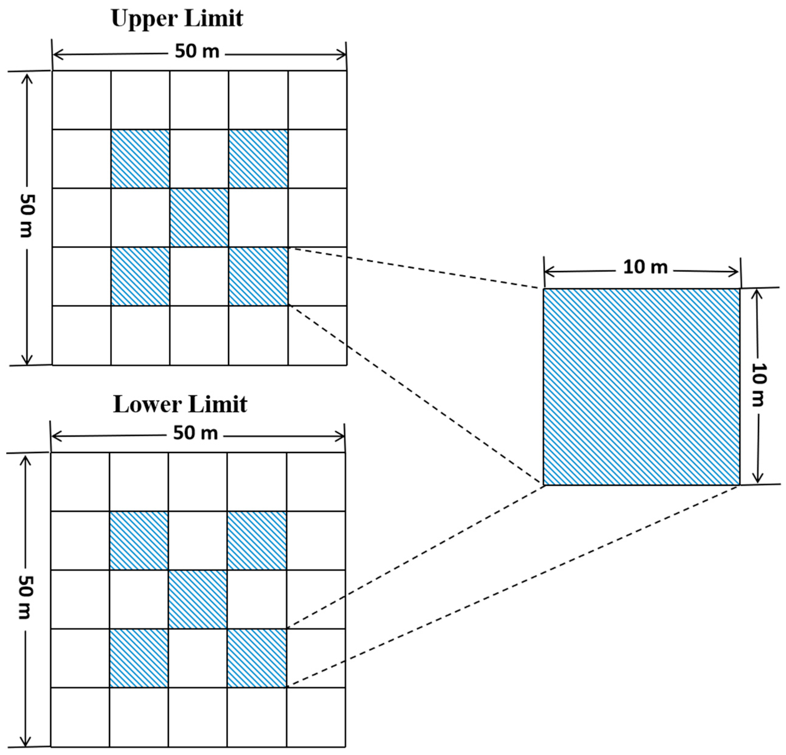
Five 10 m × 10 m quadrats were established in each sampling plot, with four quadrats located at midpoints from the midpoint of the sampling plot to four corners, and one quadrat was the midpoint of the sampling plot (Figure 2). Elevation was measured by Handy GPS in two plots; slope and slope aspect were measured by compass in each quadrate; temperature and pH of surface soil layer (0–10 cm) were measured by a handheld pH meter; an earth borer measured soil layer thickness, a steel ruler measured litter layer thickness, and tree coverage was estimated by canopy projection percentage at noon. In the case of a community survey, the interest objects of the community were tree and shrub layers. Vegetation below 5 m with no obvious main stem was defined as a shrub (Technical guidelines for biodiversity monitoring—terrestrial vascular plants from National Environmental Protection Standards of the People’s Republic of China). Therefore, tree coverage, quantity, and DBH (diameter at breast height) were recorded in the tree layer, and the height, coverage, and quantity of shrubs were recorded in the shrub layer.
More than 90% of the tree layer was constituted of P. armandii, B. albo-sinensisis, and B. utilis; therefore, the three species were chosen as target species for population development and spatial point pattern analysis. It identified and recorded DBH and coordinates of all independent trees with a diameter of at least 1 cm at breast height (DBH) in the three species by measuring tape [37]. DBH was for population development analysis, and coordinates of the three species were obtained for the spatial point pattern analysis. We divided the sampling plot (50 m × 50 m) into grids (10 m × 10 m) and measured each location in the grids with measuring tape. Finally, individual locations in 10 m × 10 m were converted to coordinates of individuals in 50 m × 50 m (Figure 2).

2.2. Data Analysis

2.2.1. Environmental Factors Analysis

Slope, soil layer thickness, litter layer thickness, pH, the temperature of the surface soil layer, and tree coverage were surveyed in the five quadrats of each sampling plot. An unpaired t-test was used to test differences for the above factors between the two limits at the p < 0.05 level. The slope aspect and elevation were measured in the centre of the 50 m × 50 m sampling plot. The number of dead trees in the 50 m × 50 m sampling plot was also recorded.

2.2.2. Importance Value Calculation

Species in different layers (tree and shrub) have different ecological functions, and the importance value was used to evaluate species status, with importance value equations as follows [38]:
Importance value (tree) = (relative coverage + relative abundance + relative dominance)/3
Importance value (shrub) = (relative height + relative coverage + relative abundance)/3
Mean importance value = Sum of importance values from all five quadrats/5
Relative abundance = Quantity of individuals of a given species/Total quantity of individuals of all species
Relative dominance = Dominance of a species/Total dominance of all species
Relative coverage = Coverage of a species/Coverage of total species
Relative height = Average height of a species/Average height of all species.

2.2.3. Community Similarity Analysis

PERMANOVA was used to carry out a community similarity test separately in the tree and shrub layers between two sampling plots. First, the Bray–Curtis dissimilarity was calculated by using the importance value of every species in the quadrats, which is a good tool for community composition analysis. Then, the “Pseudo-F statistic” method was used to test the similarity difference in two sampling plots based on the Bray–Curtis dissimilarity values.
The Bray–Curtis dissimilarity [39] (Anderson 2001):
d i , j = i = 1 k y i , k y j , k i = 1 k y i , k + y j , k
where i and j are two quadrat codes, y is the species importance value, and k is the total species richness of two quadrats, and different layers have different k values.
Pseudo F = S S B / t 1 S S W / N t
where SSB is the sum of squares between groups, SSW is the sum of squares within groups, t is the number of groups, and N is the number of total samples.

2.2.4. DBH Distribution Analysis

To assess the status of population development in the survey area, DBH data from the sampling plots were used. The DBH of every individual that met diameter criteria was recorded, with categories designated at diameters of 5 cm, 10 cm, 20 cm, and 30 cm to divide the DBH values into five bins. The quantity of individuals of each species for each DBH bin was also recorded.

2.2.5. Point Pattern Analysis

The theory of the spatial point process has been widely used to fit the specific real distribution of corresponding species by adopting many ecological hypothesis models. Considering the community traits in this study, we decided to choose four null models (complete spatial randomness, heterogeneous Poisson process, and homogeneous Thomas process, inhomogeneous Thomas process) for analysis. The pair-correlation function g(r) was calculated for each analysis. Univariate pair correlation is defined as the expected point density at distance r from a typical point of the pattern, relative to the intensity λ of the pattern [40]. It is related to the K function, whereby:
g r = d K r / d r × 2 π r
g 12 r = d K 12 r / d r × 2 π r
where K(r) is defined as the ratio of the expected number of the other points to the point density of the sample within a circle with an arbitrary point as the centre and radius r [41]. The univariate g(r) was used in the analysis of a single species. When the value of g(r) is larger than 1, the individuals in the sample have an aggregated distribution at distance r. When the value of g(r) is smaller than 1, individuals are regularly distributed at distance r. When the value of g(r) is equal to 1, individuals are randomly distributed at distance r. g(r) could extend to bivariate functions g12(r), which describes the association (interaction) between two different types of species; values of the g12(r) function that significantly deviates from 1 indicate a significant attraction (or repulsion) between the two types of points [42] (Dixon 2002). When g12(r) > 1, it shows a positive correlation; when g12(r) = 1, it shows no correlation, and when g12(r) < 1, it shows a negative correlation.
K r = A n 2 i = 1 n j = 1 n 1 w i j I r u i j   ( i j )
K 12 r = A n 1 n 2 i = 1 n 1 j = 1 n 2 1 w i j I r u i j   ( i j )
A is the area of the sampling plot, n indicates the total point in the sampling plot, r is the distance between two points, u i j is the distance between i and j when u i j < r , I r u i j = 1 , or u i j > r ,   I r u i j = 0 ; w i j indicates the ratio of a circle with i as the centre point and u i j as the radius to A.
For a single species or pair species, the pair correlation function in the null model for ecological process analysis was performed. The Monte-Carlo approach was applied to test significant g(r) values at the r scale. Each of the n = 199 simulations of a point process underlying the null model generated a summary statistic (e.g., a pair correlation function g12(r); simulation envelopes with α = 0.01 were calculated in the 199 simulations) [43]. A significant departure from the null model occurred at scale r if the test statistic was outside the simulation envelopes. This approach allowed us to approximately assess scale effects for illustrative purposes and to determine the type of significant effect. The complete spatial randomness process, Heterogeneous Poisson process, Homogeneous Thomas process, and Inhomogeneous Thomas process were used as null models [37,44,45,46].

2.2.6. Model Test

To avoid problems caused by simultaneous inference [47], we evaluated the overall ability of a given null model to describe the data by means of a goodness-of-fit test (GoF) [48]. A GoF was used to test whether a given null model fit a given summary statistic of the observed data over a given distance interval (rmin, rmax) [48]. The ui statistics were calculated for the observed data (i = 0) and simulated data (i = 1, …, 199), and the rank of u0 among all ui was determined. If the rank of u0 was larger than199, then the data showed a significant departure from the null model (across the distances of interest) with the error rate p < 0.05.

2.3. Software Analysis and Figure Processing

The “adonis2” function in the “vegan” package was applied for the PERMANOVA test for determining community composition differences. The “t.test” function in the “stats” package was applied for the analysis of the environmental factors between sites. The “Spatstat” package was applied for the analysis of spatial point pattern analysis. All analyses and the figures were plotted in R Project 3.4.3 (R Core Development Team 2017).

3. Results

3.1. Environmental Conditions within Sampling Plots

The lope difference was significant (p < 0.05), and other environmental factors differences were not significant; soil layer thickness, litter layer thickness, pH of the surface soil layer, and tree coverage were greater at the upper limit than at the lower limit. Still, the surface soil layer temperature was greater at the lower limit (Table 1).

3.2. Community Structure and Dynamic

3.2.1. Composition and Similarity Differences in Tree Layer and Shrub Layer

We detected significant differences in community composition in the tree layer, but no significant differences in the shrub layer between the upper and lower limits were found. There were five tree species and six shrub species at both limits of the treeline patch, and the average importance values of P. armandii and B. utilis were separately at the largest at the upper limit and lower limit, followed by B. albo-sinensis at both limits. In addition, Cerasus clarofolia, B. albo-sinensis, and Salix wallichiana were observed in both tree and shrub phenotypes. The B. albo-sinensis shrubs had a greater importance value than the shrubs of most other species, especially at the upper limit (Table 2).

3.2.2. DBH Numerical Distribution

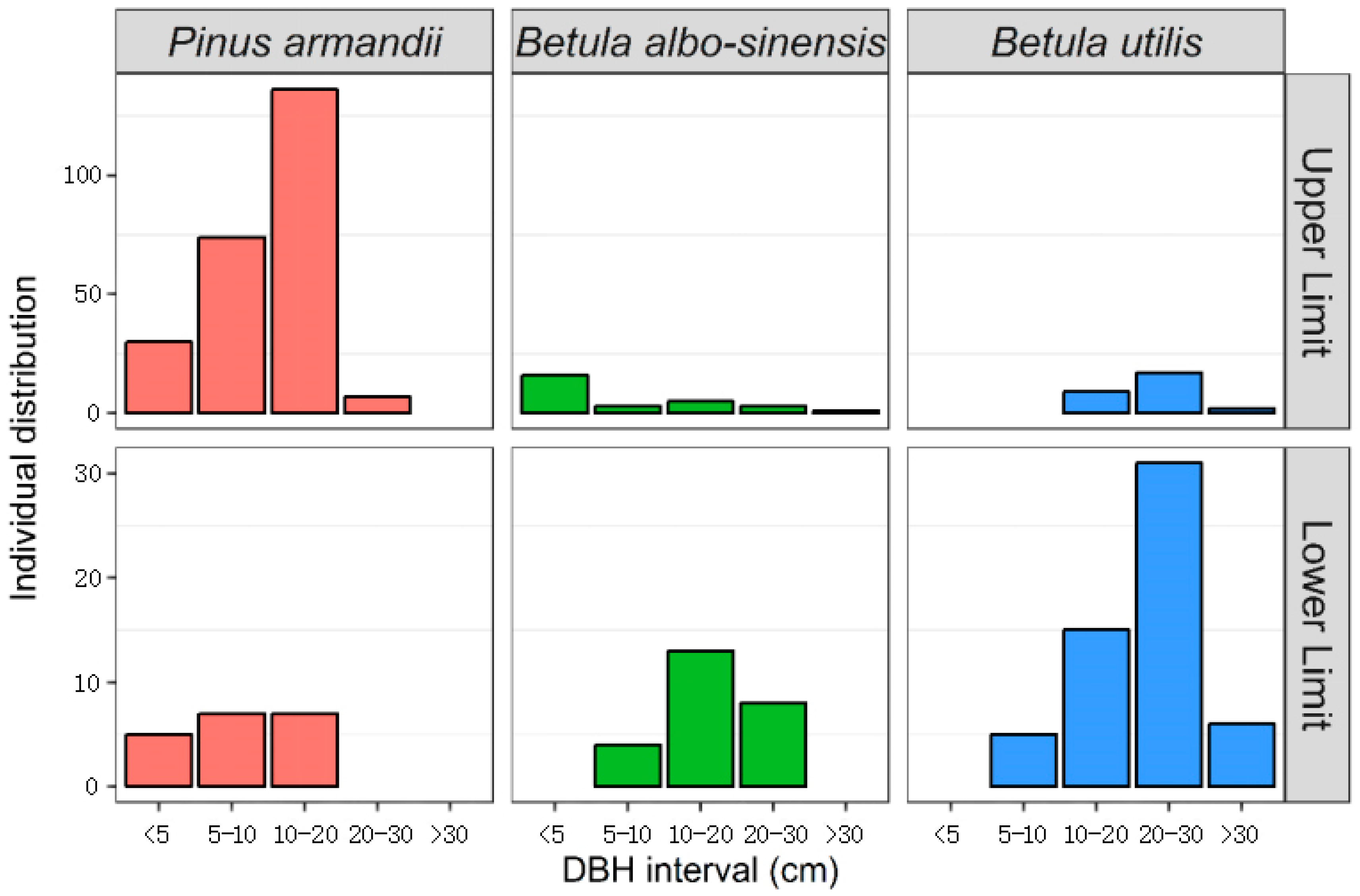
The individual distributions in Figure 3 show that the population of P. armandii was greatest at the upper limit, and that B. utilis had the largest quantity at the lower limit. The interval of 10 cm ≤ D ≤ 20 cm was the common DBH range for the three species. Pinus armandii was concentrated in a smaller DBH interval; most individual DBH values of P. armandii were distributed within the range of 10 cm ≤ D ≤ 20 cm at the upper and lower limits. The DBH values of B. albo-sinensis appeared in every DBH bin, the largest quantity of individual DBHs having D ≤ 5 cm at the upper limit, DBH values of B. albo-sinensis distributed within the range of 5 cm ≤ D ≤ 30 cm at the lower limit. Betula utilis was concentrated in larger DBH intervals (10 cm ≤ D ≤ 30 cm) at both limits, with a larger number at the lower limit than at the upper limit and individual DBHs having 5 cm ≤ D ≤ 10 cm only at the lower limit.

3.3. Null Model Analysis on Patterns, Processes of the Three Species

3.3.1. Completely Spatially Random Null Model Analysis

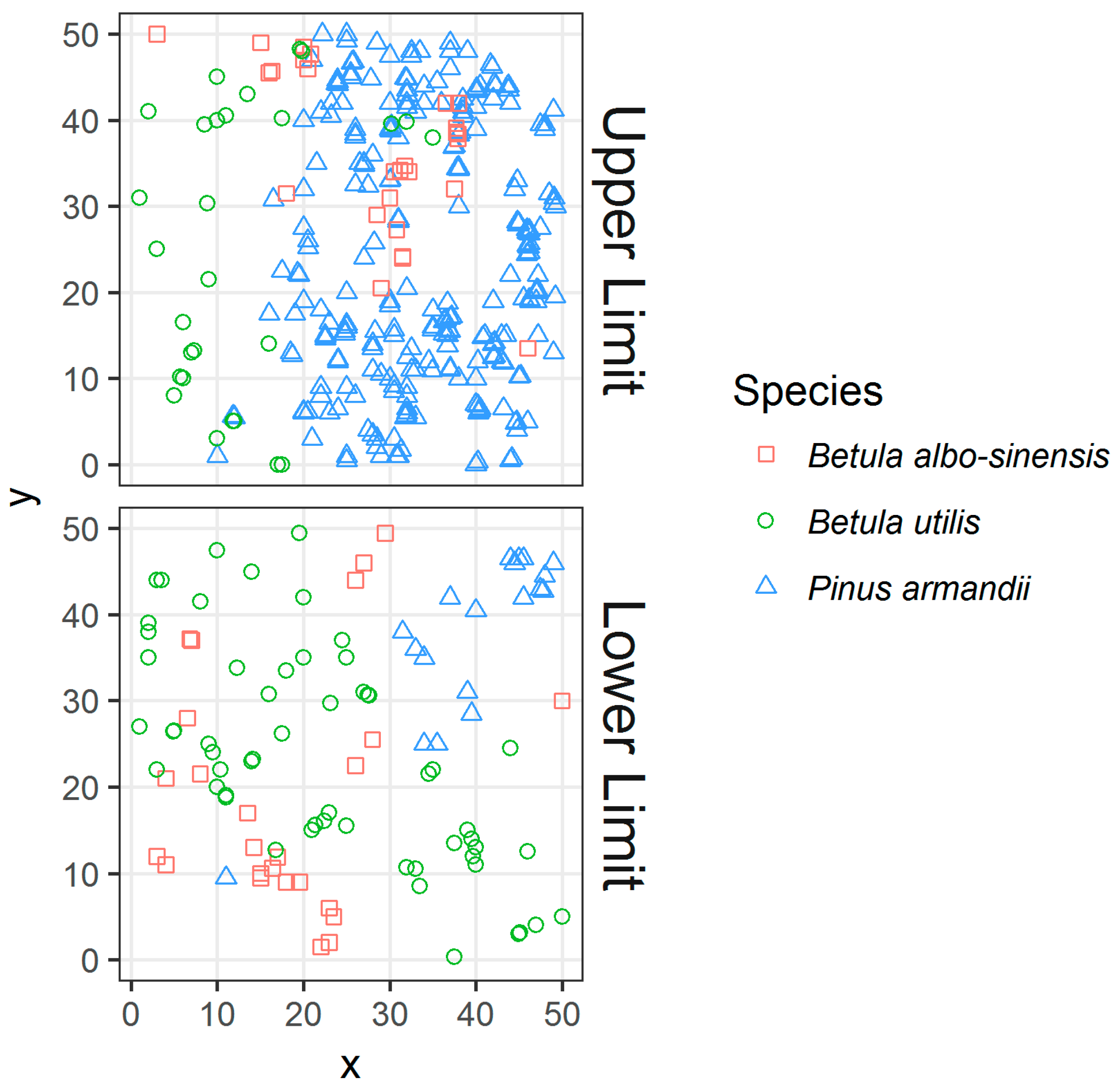
The spatial distributions of three dominant species were as shown in Figure 4. Pinus armandii distributed more on the upper limit of the treeline patch, and its aggregation area was larger. The distribution of B. albo-sinensis and B. utilis on the upper and lower limits of the treeline patch were scattered, and both their aggregation area were small. The distribution of the three species in the sampling plot did not indicate much overlap.
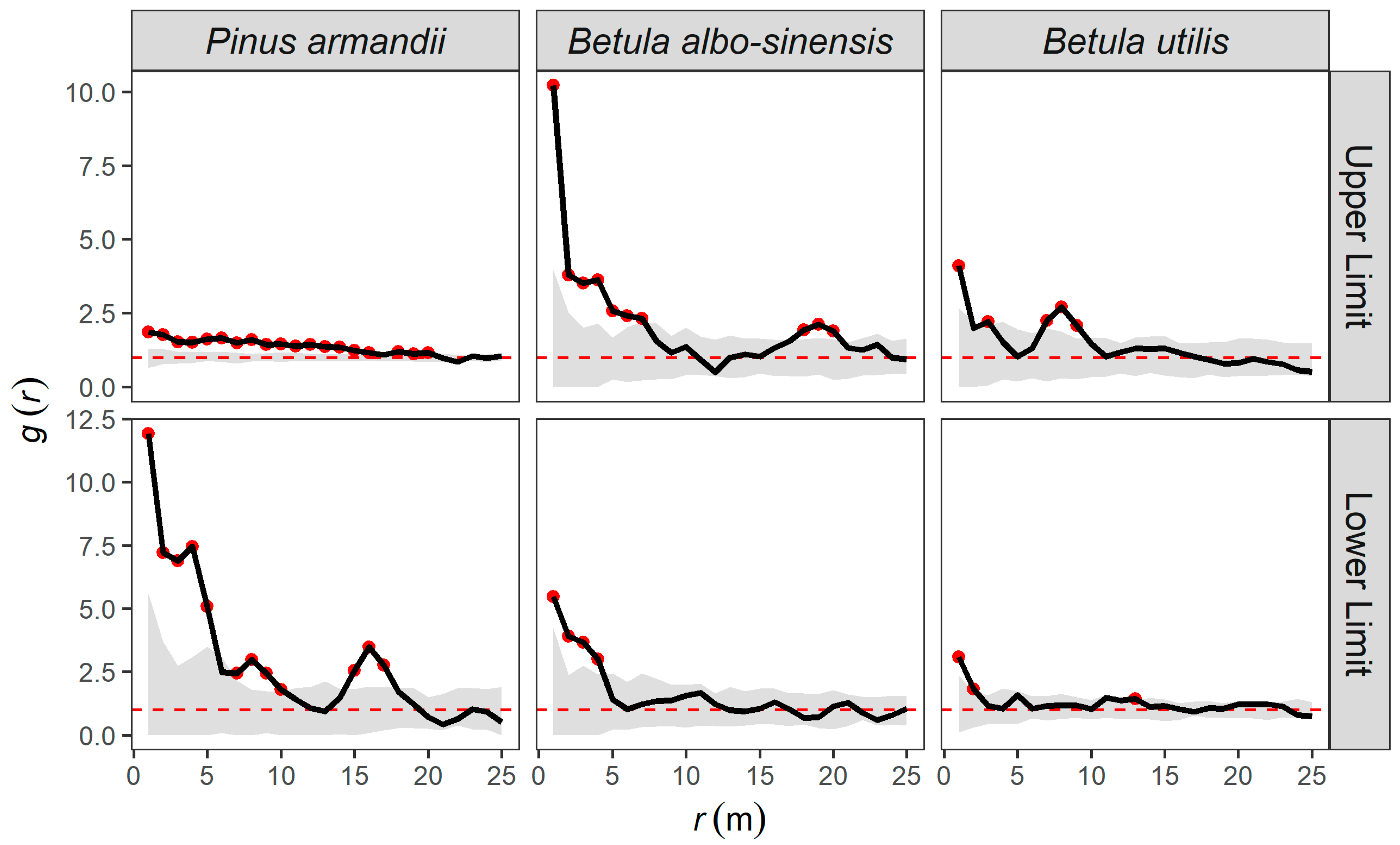
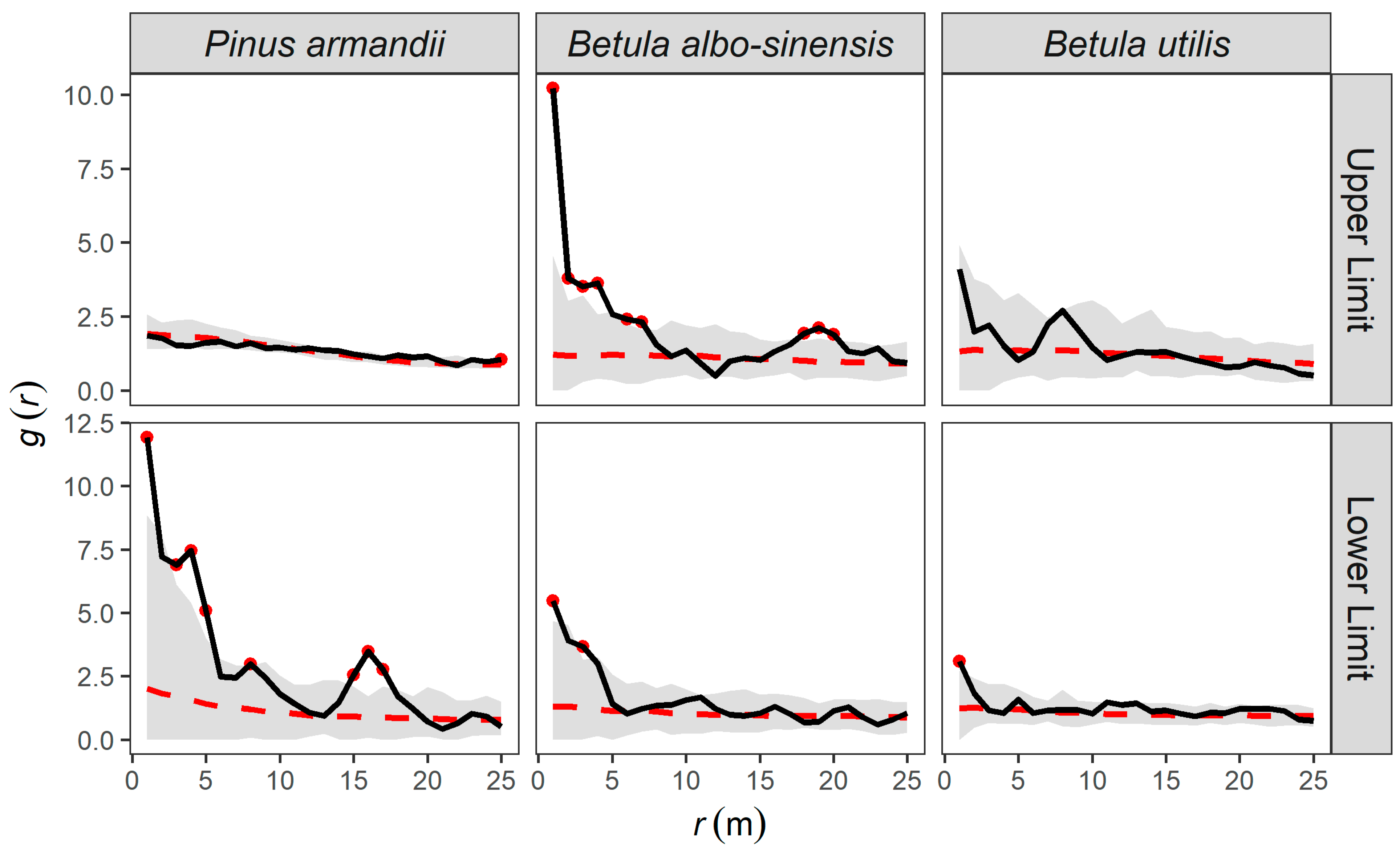
In comparing the real g(r) values with the envelope g(r) values and GoF test results (Table 3), the results were as follows: There are more real g(r) values beyond the upper envelope at the upper limit than those at the lower limit for P. armandii and B. albo-sinensis, while the g(r) values of B. utilis beyond the upper envelope were less. There are a few points at r < 10 m on the upper limit and at r < 15 m on the lower limit. The aggregation of P. armandii occurred on the broadest scales, Betula albo-sinensis aggregated at the second-broadest scale, and aggregation of B. utilis occurred at the smallest scale (Figure 5). The CSR could not fit the real patterns of the three species well (p = 0.005).

3.3.2. Heterogeneous Poisson (HP) Null Model Analysis

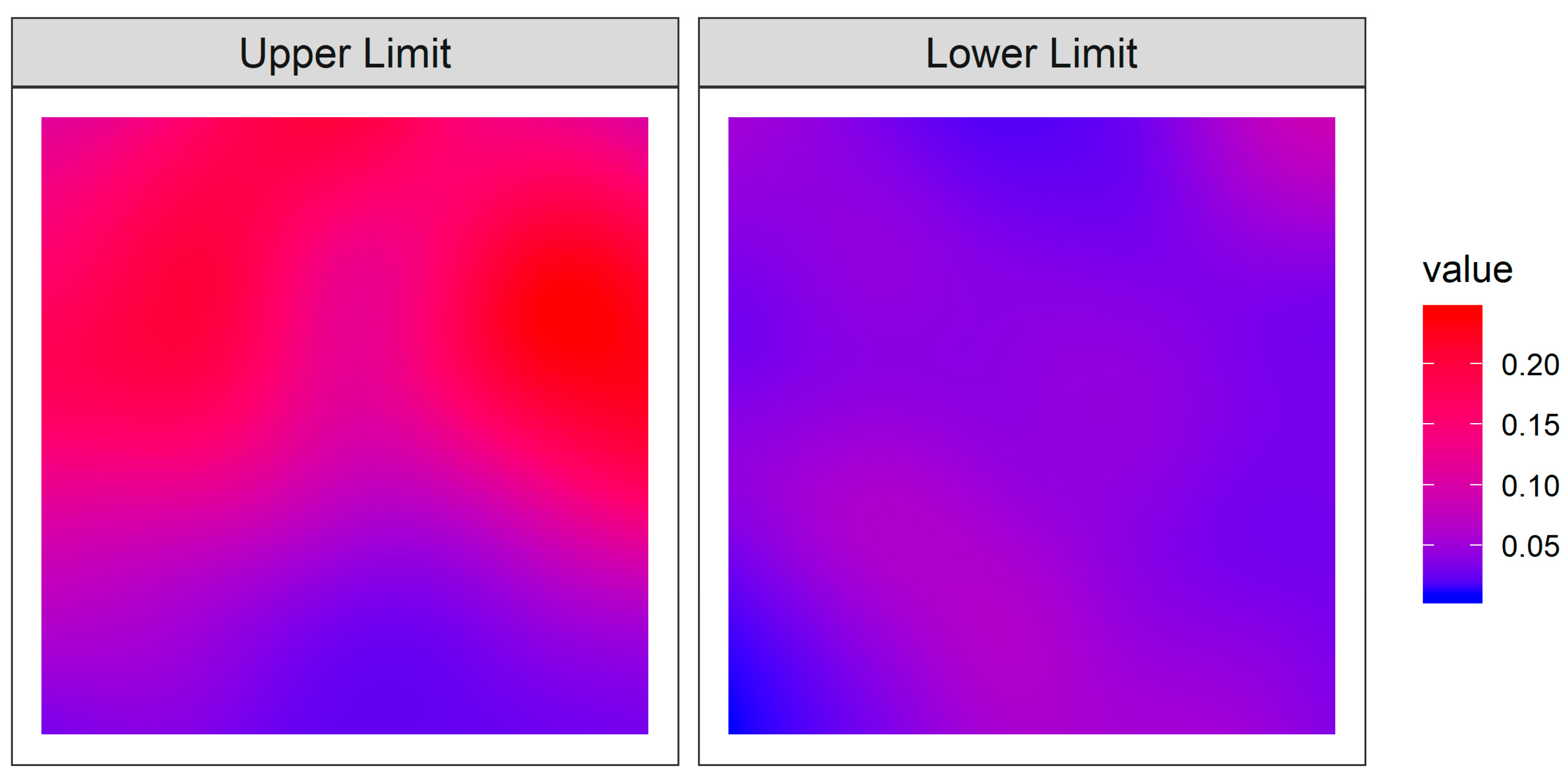
Environmental factors produced no significant differences between the upper and lower limits (Table 1). In reference to density in Figure 6, the three species’ densities were selected as background information to simulate heterogeneity.
At the upper limit, the GoF test results in Table 3 and comparisons between the real values with expected values in Figure 7 show that B. albo-sinensis and B. utilis have many g-values beyond the upper envelope, and the result of the GoF test (p < 0.05) showed their expected lines were quite different from the actual lines at 0–25 cm. While the total actual line of P. armandii was surrounded by envelopes and had a similar tendency at 0–25 m at the upper limit, the GoF test value (p = 0.115) also showed that the HP simulated pattern was not significantly different from the real pattern of P. armandii at 0–25 m on the upper limit. However, at the lower limit, the actual lines of the three species were significantly different from simulated lines at 0–25 m, respectively (p < 0.05).

3.3.3. Homogeneous Thomas (HT) Null Model Analysis

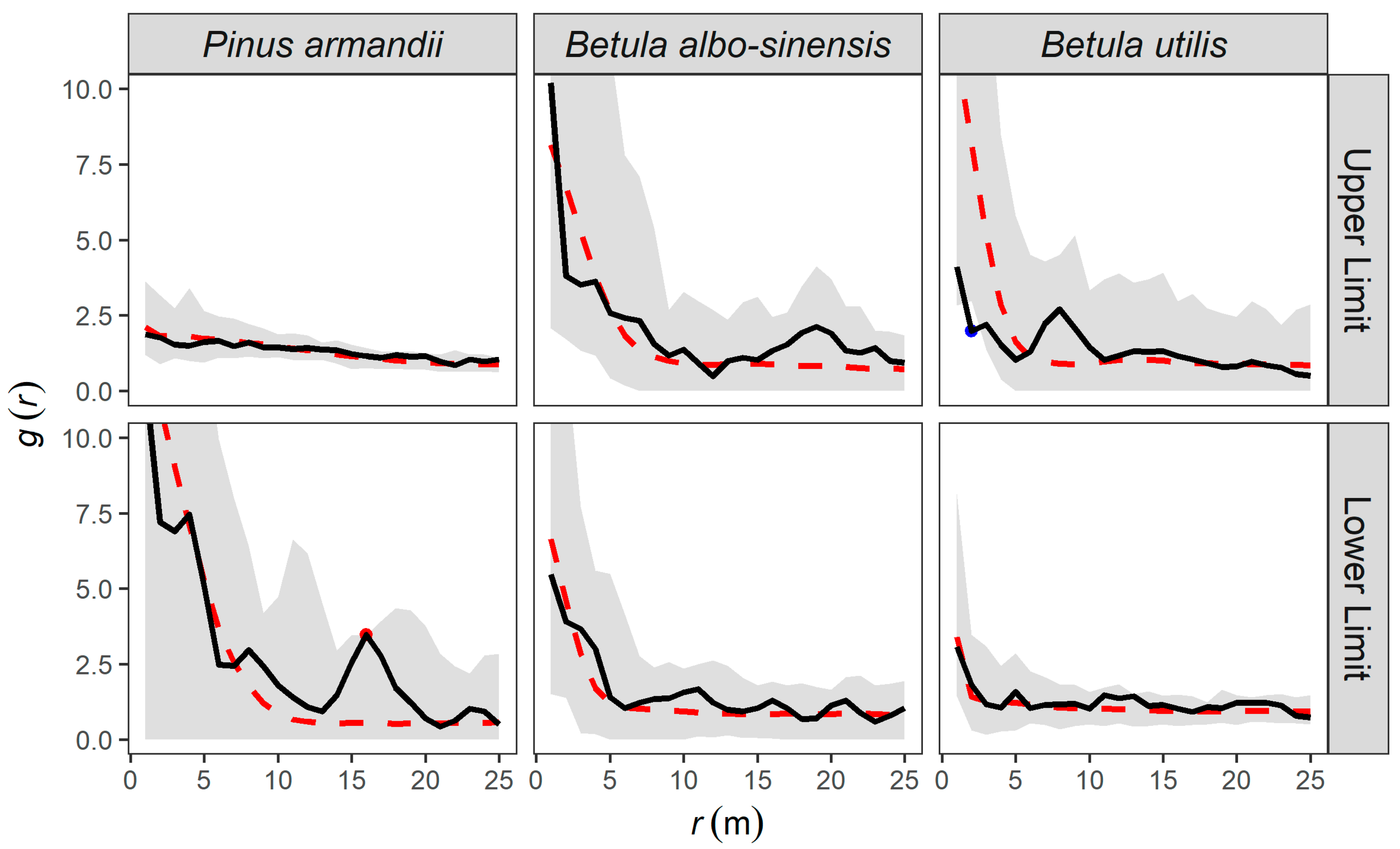
Observations from g(r) values and GoF test values (Table 3) showed the difference between the observed line and fitted expected line was significant (p < 0.05) only for P. armandii at the upper limit, where many of the g(r) values of P. armandii were greater than g-values of the upper envelopes at r < 15 m scales. The results of the GoF test at the lower limit were not significant for P. armandii (p = 0.675). The observed lines of B. albo-sinensis and B. utilis were all located inside the envelopes in both sampling plots, and the differences between their observed lines with corresponding expected lines were not significant from 0–25 m with the GoF test values (p > 0.05) (Figure 8).

3.3.4. Inhomogeneous Thomas (IT) Null Model Analysis

Most observed g(r) values were included in the 99% confidence interval for the three species, the real g(r) values of B. utilis were smaller than g(r) values of lower envelope at r = 2 m and real g(r) values of P. armandii were greater than g(r) values of the upper envelope at r = 16 m (Figure 9). GoF test values in Table 3 showed that the differences between their observed lines with the corresponding expected lines for three species were not significant at the 0–25 m scale at both the upper and lower limits (p > 0.05).

3.4. Homogeneous Poisson Null Model Analysis Inter-Specific Correlation

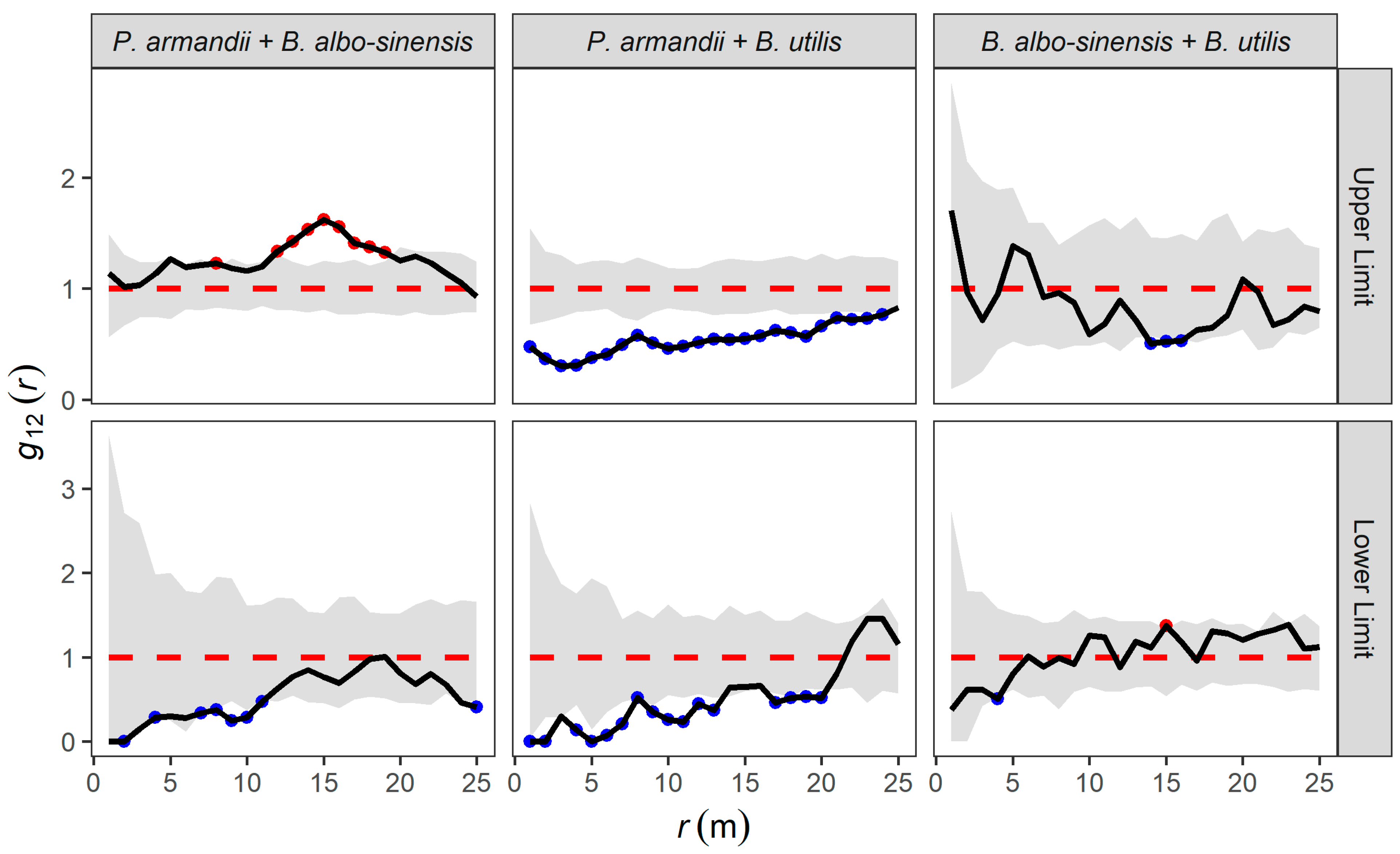
As for the upper limit, the real g12(r) values for P armandii and B. albo-sinensis were greater than the g12(r) values on the upper envelope at 10–17 m. The real g12(r) values for P. armandii and B. utilis were smaller than the g12(r) values on the lower envelope at a total 0–25 m. The real g12(r) values for B. albo-sinensis and B. utilis were smaller than the g12(r) values on the lower envelope only at a few scales of 10 m < r < 15 m (Figure 10).
As for the lower limit, the real g12(r) values for P. armandii and B. albo-sinensis were smaller than the g12(r) values on the lower envelope at r < 10 m and r = 25 m. The real g12(r) values for P. armandii and B. utilis were smaller than the g12(r) values on the lower envelope at 0–20 cm, and the significant g12(r) values were fewer than those at the upper limit of treeline patch. The real g12(r) values for B. albo-sinensis and B. utilis were greater than the g12(r) values on the upper envelope at r = 15 m (Figure 10).
The results showed that P. armandii and B. albo-sinensis had significantly positive correlations at the upper limit but a significantly negative correlation at the lower limit. Pinus armandii and Betula utilis had significantly negative correlations at both limits, and B. albo-sinensis and B. utilis had significant correlations on few scales.

4. Discussion

4.1. The Differences of Community Structure and Species Spatial Pattern at the Upper and Lower Limits of Treeline Patch

Slope differences were significant between the upper and lower limits of the treeline patch (Table 1, p < 0.05); there was significant differences in the community structure in the tree layer, but not in the shrub layer; it was not consistent with the evidence that slope had significant effects on the shrub and herbage [49,50]. In the tree layer, community structure was mainly attributed to three dominant species (P. armandii, B. albo-sinensis, and B. utilis)—they were at different statuses and stages of population development. Pinus armandii was a developing population—most of its DBH was distributed on a scale of smaller than 20 cm; the abundance of P. armandii was greater at the upper limit than that at the lower limit, which showed that population size was greater at the upper limit than that at the lower limit. The reason might be that the highly viable seeds of P. armandii help it survive in occasionally benign conditions [51]; in addition, by comparing the environmental factors of upper limit and lower limit. We also noticed that even the differences in soil thickness, litter thickness, and tree coverage were not significant, but they were superior at the upper limit to that at the lower limit (Table 1). The DBH of B. albo-sinensis distributed on a scale of smaller than 5 cm at the upper limit than that at the lower limit, population structure tended to be younger individuals. More individuals with shrub lifeform were at the upper limit, the shrub phenotype of B. albo-sinensis was a harm avoidance strategy in a stressful habitat [52]. All DBH of B. utilis was greater than 5 cm, and few shrub individuals were at the lower limit; hence, the reason might be that the recruitment and regeneration in recent years were scarce at the upper and lower limits [53]. Hence, the lifeforms and population development of the three species affected community structure in tree layers.
The occurrence scales of the three species aggregation patterns were all greater at the upper limit than those at the lower limit. Pinus armandii had the broadest aggregation scale over that of B. albo-sinensis and B. utilis. Most of the P. armandii and B. albo-sinensis were both young individuals at the upper limit, where crowded young individuals initially promoted each other’s survival and development [54]. The mutual benefits in their own populations were important for surviving in harsh environments [55]. Most individuals of the B. utilis were old trees, and it had a tolerance for low temperatures and poor habitat; hence, its pattern was a random distribution at most scales [56].
The above results accorded to our first hypothesis, and slope as an environmental factor differed significantly. Community structure and spatial pattern also had significant differences between the upper and lower limits.

4.2. Effect of Community Density Heterogeneity on Seedling Pattern

Environmental heterogeneity simulated by the density of the three species had a significant effect on the pattern of P. armandii at the upper limit; the population of P. armandii consisted mostly of medium individuals at the two limits, they were more sensitive to their surroundings [44], such as soil temperature, summer drought, and competition between the shrubs affected their survival in the treeline [57,58]. More small individuals of P. armandii were at the lower limit, and more small individuals of B. albo-sinensis were at the upper limit, but the community heterogeneity had insignificant effects on their patterns; hence, we speculated that medium tree patterns were more sensitive to density heterogeneity, which was inconsistent with the second hypothesis.

4.3. Seed Dispersal Effect and Size Effect on Species Patterns

Simulated seed dispersal of P. armandii in homogeneous conditions differed significantly from its real pattern at the upper limit; high vegetation density was an important restriction factor for seed regeneration [57]. Simulated inhomogeneity seed dispersal could well explain the patterns of three species. The pattern of the P. armandii simulated by heterogeneity and seed dispersal simultaneously could especially explain the real pattern. Pinus armandii only had seed propagation in its life history; seed productivity and dispersal were important ecological processes for population development [59], which were impeded by species distributions and the habitat conditions around it, as death density dependency [60,61] and environmental stress theory [62] stated. Hence, integrating heterogeneity characteristics and seed dispersal processes could have fitted the three species’ patterns well in our study.
The larger individuals of B. utilis distributed in the limits and competitive relationships among the canopy trees played a key role in generating stand structure [63]. The significant negative correlations between P. armandii and B. utilis occurred at both limits; this was also the case with B. albo-sinensis and B. utilis. Previous studies in the mixed forests of the Qinling Mountains suggested that less intense bamboo could impede Betula regeneration [64]; hence, both P. armandii and B. albo-sinensis had an impact on the regeneration of B. utilis.
While the correlation between B. albo-sinensis and P. armandii was positive at the upper limit and negative at the lower limit. At the upper limit, most individuals of B. albo-sinensis were smaller than P. armandii; the inverse situation happened at the lower limit. The size-adjusted inter-specific correlation, when the neighbouring species were larger than the target species, had a positive effect on it at first, then a negative effect when the neighbour species’ size reached a certain scale [62]. In addition, the DBH differences between P. armandii and B. utilis were obvious in both limits—the size effect leads to negative correlations between them [62].
As the third hypothesis stated that seed dispersal had significant effects on species patterns, the differences in size affected the inter-specific correlation, with a negative correlation often occurring between two species with a greater size difference.

5. Conclusions

Community composition in the tree layer varied significantly. The environmental factors we measured demonstrated that the slope significantly differed between the upper limit and the lower limit of the highest treeline patch. Pinus armandii had a greater population size at the upper limit, and B. utilis had a greater population size at the lower limit. The aggregation scales were greater at the upper limit for all three species. The density heterogeneity impacted the P. armandii spatial pattern at the upper limit with most of the medium individuals in its population. Inhomogeneity seed dispersal processes significantly affected the patterns of B. albo-sinensis, B. utilis and P. armandii at both limits. Pinus armandii and Betula albo-sinensis had negative interspecific correlations, which often occurred between the species with obviously different sizes. Density, seed dispersal, and unbalanced size structure played important roles in treeline patch development.
For the non-altitudinal tree line area, the slope is an important environmental factor that restricts the forest line community, and there are differences between the upper and lower limits for tree communities in the tree line. At the upper limit of the tree line, P. armandii regenerated quickly, and its population is in its development stage. Due to the population density and interspecific relationship affecting its survival, it can be considered to properly decrease the number of individuals. The young trees of B. utilis regenerate slowly—according to the existing literature, B. utilis are common constructive species in a tree line, and they could create a better living environment for other species. However, larger individuals restrict the survival of other species, so they can be planted under harsh conditions with less vegetation. The scale and size had significant effects on the relationships between the species by considering the differences in individual size and planting distance among the species. In addition, interspecific competition at some scales and some growth stages can be avoided. Seed dispersal is an important ecological process for the natural breeding of offspring, and even in harsh environments, seed dispersal characteristics should be considered for population development.

Author Contributions

M.J. participated in the fieldwork, data analysis and writing the article; J.Z. reviewed the experiment design and writing of the article; Z.S. provided suggestions on article organization. S.S. helped revise the manuscript. All authors have read and agreed to the published version of the manuscript.

Funding

This work was supported by the National Natural Science Foundation of China under Grant 31170494, the East China University of Technology Research Foundation for Careers, a special project under Grant DHBK2019103, and the East China University of Technology Research Foundation for Advanced Talents under Grant DHBK2019106.

Institutional Review Board Statement

The article complies with ethics approval, and all authors consented to participate.

Informed Consent Statement

All authors agree with this article’s publication on plant ecology and diversity.

Data Availability Statement

The datasets used and/or analyzed during the current study are available from the corresponding author upon reasonable request.

Acknowledgments

The authors wish to acknowledge Loretta Pedersen for language editing support for this article. We also thank Jonathan Bakker for helping us with the R software application, and suggestions on the article’s logical expression, and other Master’s students in the lab for their help with the field survey.

Conflicts of Interest

The authors declare they have no known competing financial interests or personal relationships that could have appeared to influence the work reported in this paper.

References

  1. Carvalhais, N.; Forkel, M.; Khomik, M.; Bellarby, J.; Jung, M.; Migliavacca, M.; Mu, M.; Saatchi, S.; Santoro, M.; Thurner, M.; et al. Global covariation of carbon turnover times with climate in terrestrial ecosystems. Nature 2014, 514, 213–217. [Google Scholar] [CrossRef] [PubMed] [Green Version]
  2. Kullman, L. Tree line population monitoring of Pinus sylvestris in the Swedish Scandes, 1973–2005: Implications for tree line theory and climate change ecology. J. Ecol. 2007, 95, 41–52. [Google Scholar] [CrossRef]
  3. Tiwari, A.; Jha, P.K. An overview of treeline response to environmental changes in Nepal Himalaya. Trop. Ecol. 2018, 59, 273–285. [Google Scholar]
  4. Chhetri, P.K.; Bista, R.; Shrestha, K.B. How does the stand structure of treeline-forming species shape the treeline ecotone in different regions of the Nepal Himalayas? J. Mt. Sci. 2020, 17, 2354–2368. [Google Scholar] [CrossRef]
  5. Shi, C.; Masson-Delmotte, V.; Daux, V.; Li, Z.S.; Carré, M.; Moore, J.C. Unprecedented recent warming rate and temperature variability over the east Tibetan Plateau inferred from Alpine treeline dendrochronology. Clim. Dyn. 2015, 45, 1367–1380. [Google Scholar] [CrossRef]
  6. Bader, M.Y.; van Geloof, I.; Rietkerk, M. High solar radiation hinders tree regeneration above the alpine treeline in northern Ecuador. Plant Ecol. 2007, 191, 33–45. [Google Scholar] [CrossRef]
  7. Kaspar, J.; Treml, V. Thermal characteristics of alpine treelines in Central Europe north of the Alps. Clim. Res. 2016, 68, 1–12. [Google Scholar] [CrossRef]
  8. Gruber, A.; Baumgartner, D.; Zimmermann, J.; Oberhuber, W. Temporal dynamic of wood formation in Pinus cembra along the alpine treeline ecotone and the effect of climate variables. Trees-Struct. Funct. 2009, 23, 623–635. [Google Scholar] [CrossRef] [Green Version]
  9. Renard, S.M.; McIntire, E.J.B.; Fajardo, A.; Woods, K. Winter conditions—Not summer temperature—Influence establishment of seedlings at white spruce alpine treeline in Eastern Quebec. J. Veg. Sci. 2016, 27, 29–39. [Google Scholar] [CrossRef]
  10. Greenwood, S.; Chen, J.-C.; Chen, C.-T.; Jump, A.S. Strong topographic sheltering effects lead to spatially complex treeline advance and increased forest density in a subtropical mountain region. Glob. Chang. Biol. 2014, 20, 3756–3766. [Google Scholar] [CrossRef]
  11. Guo, D.; Zhang, H.-Y.; Hou, G.-L.; Zhao, J.-J.; Liu, D.-Y.; Guo, X.-Y. Topographic controls on alpine treeline patterns on Changbai Mountain, China. J. Mt. Sci. 2014, 11, 429–441. [Google Scholar] [CrossRef]
  12. Brodersen, C.R.; Germino, M.J.; Smith, W.K. Photosynthesis during an episodic drought in Abies lasiocarpa and Picea engelmannii across an alpine treeline. Arct. Antarct. Alp. Res. 2006, 38, 34–41. [Google Scholar] [CrossRef] [Green Version]
  13. Stueve, K.M.; Cerney, D.L.; Rochefort, R.M.; Kurth, L.L. Post-fire tree establishment patterns at the alpine treeline ecotone: Mount Rainier National Park, Washington, USA. J. Veg. Sci. 2009, 20, 107–120. [Google Scholar] [CrossRef]
  14. Adhikari, B.S.; Kumar, R.; Singh, S.P. Early snowmelt impact on herb species composition, diversity and phenology in a western Himalayan treeline ecotone. Trop. Ecol. 2018, 59, 365–382. [Google Scholar]
  15. Pereg, D.; Payette, S. Development of black spruce growth forms at treeline. Plant Ecol. 1998, 138, 137–147. [Google Scholar] [CrossRef]
  16. D’Arrigo, R.; Jacoby, G.; Buckley, B.; Sakulich, J.; Frank, D.; Wilson, R.; Curtis, A.; Anchukaitis, K. Tree growth and inferred temperature variability at the North American Arctic treeline. Glob. Planet. Chang. 2009, 65, 71–82. [Google Scholar] [CrossRef]
  17. Dawes, M.A.; Haettenschwiler, S.; Bebi, P.; Hagedorn, F.; Handa, I.T.; Köerner, C.; Rixen, C. Species-specific tree growth responses to 9 years of CO2 enrichment at the alpine treeline. J. Ecol. 2011, 99, 383–394. [Google Scholar] [CrossRef]
  18. Barbeito, I.; Bruecker, R.L.; Rixen, C.; Bebi, P. Snow Fungi-Induced Mortality of Pinus cembra at the Alpine Treeline: Evidence from Plantations. Arct. Antarct. Alp. Res. 2013, 45, 455–470. [Google Scholar] [CrossRef] [Green Version]
  19. Hiemstra, C.A.; Liston, G.E.; Reiners, W.A. Snow redistribution by wind and interactions with vegetation at upper treeline in the Medicine Bow Mountains, Wyoming, USA. Arct. Antarct. Alp. Res. 2002, 34, 262–273. [Google Scholar] [CrossRef]
  20. Hattenschwiler, S.; Smith, W.K. Seedling occurrence in alpine treeline conifers: A case study from the central Rocky Mountains, USA. Acta Oecolog.-Int. J. Ecol. 1999, 20, 219–224. [Google Scholar] [CrossRef]
  21. Hughes, N.M.; Johnson, D.M.; Akhalkatsi, M.; Abdaladze, O. Characterizing Betula litwinowii Seeding Microsites at the Alpine-Treeline Ecotone, Central Greater Caucasus Mountains, Georgia. Arct. Antarct. Alp. Res. 2009, 41, 112–118. [Google Scholar] [CrossRef]
  22. Germino, M.J.; Smith, W.K.; Resor, A.C. Conifer seedling distribution and survival in an alpine-treeline ecotone. Plant Ecol. 2002, 162, 157–168. [Google Scholar] [CrossRef]
  23. Holtmeier, F.K.; Broll, G. Sensitivity and response of northern hemisphere altitudinal and polar treelines to environmental change at landscape and local scales. Glob. Ecol. Biogeogr. 2005, 14, 395–410. [Google Scholar] [CrossRef]
  24. Elliottt, G.P.; Kipfmueller, K.E. Multi-scale Influences of Slope Aspect and Spatial Pattern on Ecotonal Dynamics at Upper Treeline in the Southern Rocky Mountains, USA. Arct. Antarct. Alp. Res. 2010, 42, 45–56. [Google Scholar] [CrossRef] [Green Version]
  25. Liptzin, D.; Sanford, R.L., Jr.; Seastedt, T.R. Spatial patterns of total and available N and P at alpine treeline. Plant Soil 2013, 365, 127–140. [Google Scholar] [CrossRef]
  26. Thebault, A.; Clement, J.-C.; Ibanez, S.; Roy, J.; Geremia, R.A.; Perez, C.A.; Buttler, A.; Estienne, Y.; Lavorel, S. Nitrogen limitation and microbial diversity at the treeline. Oikos 2014, 123, 729–740. [Google Scholar] [CrossRef] [Green Version]
  27. Jameson, R.G.; Trant, A.J.; Hermanutz, L. Insects can limit seed productivity at the treeline. Can. J. For. Res. 2015, 45, 286–296. [Google Scholar] [CrossRef]
  28. Anschlag, K.; Broll, G.; Holtmeier, F.-K. Mountain Birch Seedlings in the Treeline Ecotone, Subarctic Finland: Variation in Above- and Below-Ground Growth Depending on Microtopography. Arct. Antarct. Alp. Res. 2008, 40, 609–616. [Google Scholar] [CrossRef] [Green Version]
  29. Brooker, R.W.; Scott, D.; Palmer, S.C.F.; Swaine, E. Transient facilitative effects of heather on Scots pine along a grazing disturbance gradient in Scottish moorland. J. Ecol. 2010, 94, 637–645. [Google Scholar] [CrossRef]
  30. Brooker, R.W.; Callaghan, T.V. The balance between positive and negative plant interactions and its relationship to environmental gradients: A model. Oikos 1998, 81, 196–207. [Google Scholar] [CrossRef]
  31. le Roux, P.C.; McGeoch, M.A. Spatial variation in plant interactions across a severity gradient in the sub-Antarctic. Oecologia 2008, 155, 831–844. [Google Scholar] [CrossRef] [PubMed]
  32. Miao, N.; Liu, S.R.; Shi, Z.M.; Xue, Z.B.; Yu, H.; He, F. 青藏高原东缘林线杜鹃-岷江冷杉原始林的空间格局 [Spatial pattern analysis of a Rhododendron-Abies virginal forest near timberline on the eastern edge of Qinghai-Tibetan Plateau, China]. Acta Ecol. Sin. 2011, 31, 1–9. [Google Scholar]
  33. Zhang, Q.Y. 青藏高原东缘高山林线乔木种群生态特征研究 [Ecological Characteristics of Timberline Tree Populations in Eastern Qinghai—Tibetan Plateau]; Graduate School, Chinese Academy of Sciences: Chengdu, China, 2006. [Google Scholar]
  34. Wang, H.T. 山西历山自然生态风景区的开发利用 [Development and Utilization of Li Mountain Natural Ecological Scenic Area in Shanxi Province]. Shanxi Agric. Econ. 2017, 5, 69–71. [Google Scholar] [CrossRef]
  35. Ru, W.; Zhang, J.T.; Zhang, F.; Zhang, G.; Liu, R. 历山森林群落物种多样性与群落结构研究 [Species diversity and community structure of forest communities in Lishan Mountain]. Chin. J. Appl. Ecol. 2006, 17, 561–566. [Google Scholar] [CrossRef]
  36. Ru, W.M.; Zhang, F. 山西中条山东部种子植物区系分析 [Analysis on the flora of eastern Zhongtiao Mountains, Shanxi]. J. Shanxi Univ. 2000, 23, 82–87. [Google Scholar] [CrossRef]
  37. Wang, X.G.; Wiegand, T.; Hao, Z.Q.; Li, B.H.; Ye, J.; Lin, F. Species associations in an old-growth temperate forest in north-eastern China. J. Ecol. 2010, 98, 674–686. [Google Scholar] [CrossRef]
  38. Nguyen, H.; Lamb, D.; Herbohn, J.; Firn, J. Designing Mixed Species Tree Plantations for the Tropics: Balancing Ecological Attributes of Species with Landholder Preferences in the Philippines. PLoS ONE 2014, 9, E95267. [Google Scholar] [CrossRef]
  39. Anderson, M.J. A new method for non-parametric multivariate analysis of variance. Austral Ecol. 2001, 26, 32–46. [Google Scholar] [CrossRef]
  40. Wiegand, T.; Moloney, K.A. A Handbook of Spatial Point Pattern Analysis in Ecology; Chapman and Hall/CRC Press: Boca Raton, FL, USA, 2014. [Google Scholar]
  41. Liang, Y.; Yang, X.X.; Zhang, X.Y.; Zhang, J.T.; Zhang, D.Y.; Liao, W.J. Effects of plant interactions on the populations of the endangered Fagus pashanica. Plant Ecol. Divers. 2022, 15, 25–37. [Google Scholar] [CrossRef]
  42. Dixon, P.M. Ripley’s K function. Encycl. Environ. 2002, 3, 1796–1803. [Google Scholar]
  43. Stoyan, D.; Stoyan, H. Fractals, Random Shapes, and Point Fields: Methods of Geometrical Statistics; John Wiley and Sons: Chichester, UK, 1994; Volume 302. [Google Scholar]
  44. Jia, M.Y.; Zhang, J.T.; Song, Z.H.; Liang, Y. Size-gradient differences in the spatial patterns and processes of Pinus armandii in forest lines of Li Mountains, North Central China. Acta Ecol. Sin. 2022, 42, 162–170. [Google Scholar] [CrossRef]
  45. Waagepetersen, R.P. An estimating function approach to inference for inhomogeneous Neyman-Scott processes. Biometrics 2007, 63, 252–258. [Google Scholar] [CrossRef] [PubMed] [Green Version]
  46. Wiegand, T.; Gunatilleke, S.; Gunatilleke, N.; Okuda, T. Analyzing the spatial structure of a Sri Lankan tree species with multiple scales of clustering. Ecology 2007, 88, 3088–3102. [Google Scholar] [CrossRef] [PubMed]
  47. Wang, X.G.; Wiegand, T.; Wolf, A.; Howe, R.; Davies, S.J.; Hao, Z. Spatial patterns of tree species richness in two temperate forests. J. Ecol. 2011, 99, 1382–1393. [Google Scholar] [CrossRef]
  48. Loosmore, N.B.; Ford, E.D. Statistical inference using the G or K point pattern spatial statistics. Ecology 2006, 87, 1925–1931. [Google Scholar] [CrossRef] [Green Version]
  49. Zhang, J.-T.; Xiang, C.L.; Li, M. Effects of Tourism and Topography on Vegetation Diversity in the Subalpine Meadows of the Dongling Mountains of Beijing, China. Environ. Manag. 2012, 49, 403–411. [Google Scholar] [CrossRef] [PubMed]
  50. Li, C.J.; Sun, Q.; Chen, Z.; Pang, L.; Long, F. 道路边坡坡度对植被恢复中物种多样性的影响研究 [Effects of Roadside Slope Gradient on Plant Diversty during Revegetation]. Bulletion Bot. Res. 2013, 33, 447–483. [Google Scholar]
  51. Dirr, M.A. Manual of Woody Landscape Plants: Their Identification, Ornamental Characteristics, Culture, Propagation and Uses, 3rd ed.; Stipes Publishing Co.: Champaign, IL, USA, 1983. [Google Scholar]
  52. Wang, X.Y.; Yu, D.P.; Zhou, L.; Zhou, W.M.; Wu, Z.J.; Guo, Y.; Bao, Y.; Meng, Y.Y.; Dai, L.M. 长白山北坡林线岳桦种群空间分布格局 [Spatial patterns of a treeline Betula ermanii Cham. population on the north slope of Changbai Mountain]. Acta Ecol. Sin. 2015, 35, 116–124. [Google Scholar] [CrossRef] [Green Version]
  53. Guo, Y.-X.; Li, G.; Hu, Y.-N.; Kang, D.; Wang, D.X.; Yang, G.H. Regeneration of Betula albosinensis in Strip Clearcut and Uncut Forests of the Qinling Mountains in China. PLoS ONE 2013, 8, e59375. [Google Scholar] [CrossRef] [Green Version]
  54. Zhang, Y.; Zhang, C.-Y.; Zhao, X.-H. 内蒙古黑里河天然油松林主要树种的空间分布格局 [Spatial Distribution Pattern of Main Tree Species in Pinus tabulae formis Forest of Heilihe in Inner-Mongolia]. Acta Bot. Boreal-Occident. Sin. 2009, 29, 167–173. [Google Scholar] [CrossRef]
  55. Jobbagy, E.G.; Jackson, R.B. Global controls of forest line elevation in the northern and southern hemispheres. Glob. Ecol. Biogeogr. 2000, 9, 253–268. [Google Scholar] [CrossRef] [Green Version]
  56. Bharti, R.R.; Adhikari, B.S.; Rawat, G.S. Assessing vegetation changes in timberline ecotone of Nanda Devi National Park, Uttarakhand. Int. J. Appl. Earth Obs. Geoinf. 2012, 18, 472–479. [Google Scholar] [CrossRef]
  57. Frei, E.R.; Bianchi, E.; Bernareggi, G.; Bebi, P.; Dawes, M.A.; Brown, C.D.; Trant, A.J.; Mamet, S.D.; Rixen, C. Biotic and abiotic drivers of tree seedling recruitment across an alpine treeline ecotone. Sci. Rep. 2018, 8, 10894. [Google Scholar] [CrossRef] [Green Version]
  58. Lett, S.; Dorrepaal, E. Global drivers of tree seedling establishment at alpine treelines in a changing climate. Funct. Ecol. 2018, 32, 1666–1680. [Google Scholar] [CrossRef] [Green Version]
  59. Kambo, D.; Danby, R.K. Constraints on treeline advance in a warming climate: A test of the reproduction limitation hypothesis. J. Plant Ecol. 2018, 11, 411–422. [Google Scholar] [CrossRef]
  60. Bai, X.J.; Queenborough, S.A.; Wang, X.G.; Zhang, J.; Li, B.H.; Yuan, Z.Q.; Xing, D.L.; Lin, F.; Ye, J.; Hao, Z.Q. Effects of local biotic neighbors and habitat heterogeneity on tree and shrub seedling survival in an old-growth temperate forest. Oecologia 2012, 170, 755–765. [Google Scholar] [CrossRef] [PubMed]
  61. HilleRisLambers, J.; Clark, J.S.; Beckage, B. Density-dependent mortality and the latitudinal gradient in species diversity. Nature 2002, 417, 732–735. [Google Scholar] [CrossRef]
  62. Malanson, G.P.; Resler, L.M. A size-gradient hypothesis for alpine treeline ecotones. J. Mt. Sci. 2016, 13, 1154–1161. [Google Scholar] [CrossRef]
  63. Šrůtek, M.; Doležal, J.; Hara, T. Spatial structure and associations in a Pinus canariensis population at the treeline, Pico del Teide, Tenerife, Canary Islands. Arct. Antarct. Alp. Res. 2002, 34, 201–210. [Google Scholar] [CrossRef]
  64. Wang, W.; Franklin, S.B.; Ren, Y.; Ouellette, J.R. Growth of bamboo Fargesia qinlingensis and regeneration of trees in a mixed hardwood-conifer forest in the Qinling Mountains, China. For. Ecol. Manag. 2006, 234, 107–115. [Google Scholar] [CrossRef]
Figure 1. Location of the study area.
Land 11 02064 g001
Figure 2. Sampling plot design.
Land 11 02064 g002
Figure 3. DBH distribution of three species at five diameter intervals (D ≤ 5 cm, 5 cm ≤ D ≤ 10 cm, 10 cm ≤ D ≤ 20 cm, 20 cm ≤ D ≤ 30 cm, D ≥ 30 cm) in the sampling plots of the treeline patch.
Land 11 02064 g003
Figure 4. Spatial distribution in the sampling plots from the upper and lower limits.
Land 11 02064 g004
Figure 5. The CSR null model analysis of the spatial patterns of the three species at the upper and lower limits of the treeline patch. Note: The black lines are the observed lines, namely the actual lines of the species patterns at 0–25 m; the red dashed lines are the expected lines; the red points are the g-values beyond the upper envelope at a corresponding scale.
Land 11 02064 g005
Figure 6. Heatmap of environmental heterogeneity indicated by the density in the sites from the upper and lower limits of the treeline patch.
Land 11 02064 g006
Figure 7. HP null model analysis of spatial patterns of P. armandii, B. albo-sinensis, and B. utilis at the upper limit and the lower limit of the treeline patch. Note: the red points are the g-values beyond the upper envelope at a corresponding scale, the blue points are the g-values under the lower envelope at a corresponding scale.
Land 11 02064 g007
Figure 8. HT null model analysis of the spatial patterns of P. armandii, B. albo-sinensis, and B. utilis at the upper limit and lower limit of the treeline patch. Note: the red points are the g-values beyond the upper envelope at a corresponding scale, the blue points are the g-values under the lower envelope at a corresponding scale.
Land 11 02064 g008
Figure 9. Inhomogeneous Thomas null model analysis of the spatial patterns of P. armandii, B. albo-sinensis and B. utilis in the sites from the upper and lower limits on treeline forest. Note: the red points are the g-values beyond the upper envelope at a corresponding scale, the blue points are the g-values under the lower envelope at a corresponding scale.
Land 11 02064 g009
Figure 10. Correlation analysis of P. armandii, B. albo-sinensis, and B. utilis at the upper limit and lower limit of the treeline patch. Note: the red points are the g-values beyond the upper envelope at a corresponding scale, the blue points are the g-values under the lower envelope at a corresponding scale.
Land 11 02064 g010
Table 1. Environmental conditions at the upper and lower limits.
Environmental FactorsUpper LimitLower LimitSignificance
Altitude (m)23002250None
Slope aspectNorth by east 45°True northNone
Number of dead trees
Slope * (°)
14
28.6 A ± 2.27
7
6.6 B ± 1.03
None
p < 0.05
Soil layer thickness (cm)27.8 ± 9.0919.0 ± 4.54p > 0.05
Litter layer thickness (cm)4.0 ± 3.391.4 ± 0.77p > 0.05
pH of surface soil layer5.9 ± 0.105.9 ± 0.15p > 0.05
Temperature of surface soil layer (°C)12.3 ± 0.9713.6 ± 0.89p > 0.05
Tree coverage (%)51.0 ± 11.4043.8.0 ± 10.50p > 0.05
Note: The values of altitude, slope aspect and the number of dead trees were measured in a 50 m × 50 m sampling plot, the others were measured in five 10 m × 10 m quadrats. “None” means this factor has not been tested for significance. * means significant difference between Upper Limit and Lower Limit. Superscript letter A and Superscript letter B are the result of t-test, it shows difference between Upper Limit and Lower Limit, A means larger value, B means smaller value.
Table 2. Average importance values and PERMANOVA test on the similarity of community composition in the tree layer and the shrub layer.
Life FormSpeciesUpper LimitLower Limit
Tree layerPinus armandii0.3610.012
p = 0.049 *Betula albo-sinensis0.3310.095
Betula utilis0.2370.804
Padus racemosa0.0340.034
Cerasus clarofolia0.0170.056
Salix wallichiana0.0200.000
Shrub layerBetula albo-sinensis0.4770.137
p = 0.31Cotoneaster acutifolius0.0730.038
Lonicera szechuanica0.0430.064
Lonicera chrysantha0.0370.079
Pertya sinensis0.0360.148
Salix wallichiana0.0320.050
Spiraea trilobata0.1000.000
Rubus flosculosus0.0630.000
Ribes vilmorinii0.0510.000
Sorbus koehneana0.0000.077
Viburnum mongolicum0.0000.062
Eleutherococcus henryi0.0000.048
Abelia biflora0.0000.032
Cerasus clarofolia0.0000.200
Note: “*” means that the similarity was significantly different at the p < 0.05 level.
Table 3. GoF test significance for Complete spatial randomness, Inhomogeneous Poisson, Homogeneous Thomas and Inhomogeneous Thomas null model fit effects.
Test ItemCSR Null ModelIP Null ModelHT Null ModelIT Null Model
Upper Limit—Pinus armandii0.0050.1150.005 **0.875
Upper Limit—Betula albo-sinensis0.0050.005 **0.4000.435
Upper Limit—Betula utilis0.0050.015 *0.3500.090
Lower Limit—Pinus armandii0.0050.005 *0.6750.510
Lower Limit—Betula albo-sinensis0.0050.010 *0.9200.805
Lower Limit—Betula utilis0.0050.020 *0.3350.710
Note: “CSR”, “IP”, “HT” and “IT” are abbreviations of Complete Spatial Randomness, Inhomogeneous Poisson, Homogeneous Thomas and Inhomogeneous Thomas, respectively. * means significant differences between the expected line simulated by the null model and the observed line at α = 0.05, ** means extremely significant differences between the expected line and the observed line at α = 0.01.
Publisher’s Note: MDPI stays neutral with regard to jurisdictional claims in published maps and institutional affiliations.