The Importance of Very-High-Resolution Imagery to Map Invasive Plant Species: Evidence from Galapagos

Abstract

Invasive species are one of the main threats to biodiversity worldwide, and the Galapagos Islands are no exception. With the need to control many invasive plant species, accurate distribution maps of invasive plant species are crucial for cost-effective management actions. To guide the selection of appropriate multispectral satellite imagery for this, we evaluated the effects that spatial resolution has on the mapping accuracy of the most invasive plant species in Galapagos with different “growth forms”: (1) tall tree: Cuban cedar (Cedrela odorata), (2) medium tree: guava (Psidium guajava), and (3) shrub: blackberry (Rubus niveus). We developed a mapping methodology based on very high resolution (VHR, WorldView-2) imagery and visual interpretation from orthophotos obtained from unmanned aerial vehicles for training and validation. We then compared our VHR mapping results with medium resolution (MR, Landsat) mapping results and calculated the overall accuracy (OA) and Kappa from confusion matrices for each target species and resolution based on the visual interpretation of Google Earth imagery. The results showed that the OA of the maps produced with VHR was significantly higher than the ones produced with MR. The OA was higher for the tall tree growth form, followed by the shrub and the medium tree growth form. Kappa estimates of <0.5 for MR for the medium tree and shrub growth forms demonstrated its unsuitability for accurate mapping. While MR may be sufficient for mapping the tall tree growth form, we concluded that VHR is indispensable for mapping the medium tree and shrub growth forms.

1. Introduction

Invasive species are a threat to global biodiversity, as they can adversely affect ecosystems by displacing native and endemic species and altering ecosystem functions [1,2]. Preserving the integrity and biodiversity of ecosystems with high conservation values requires management actions to control the spread of invasive species [3]. The costs of the economic loss due to invasive species and their control are very high on a global scale, with annual costs of an estimated USD 120 billion in the US [4], USD 14.45 billion in China [5], and up to USD 626 million over 34 years in Ecuador [6]. Since funds for controlling these species are often scarce, it is important to allocate funds to priority areas, requiring accurate species distribution maps [7]. Such maps can help establish baseline ecosystem conditions [8], localize and target early infestations [9], model invasion patterns, or monitor management outcomes [10], all of which are essential to protect ecosystems threatened by invasive species [2].

Remote sensing technologies offer an important resource for mapping vegetation [11]. Multispectral satellite images, i.e., images composed of multiple spectral bands containing the amount of radiation of a range of wavelengths, have widely been used to characterize vegetation according to its spectral properties [12,13,14]. Satellite sensors have different spatial resolutions, which are the ground representation of one pixel in the image. They range from low resolution, where a single pixel encompasses several trees or plants, to high resolution, where a tree or plant is represented by one or a few pixels [15]. Lower resolutions are often used to map vegetation communities or ecosystems, whereas higher resolutions are commonly used to map single species [16,17]. While higher resolution imagery is costlier to acquire [17] and has a lower temporal frequency and geographic coverage in tropical areas [16], it has the advantage of greater detail that enhances the recognition of features. What allows the recognition of a plant species, apart from its spectral characteristics, is a combination of several features visible from above, for example, whether the plant species forms a tree crown, large monospecific stands, small patches mixed with other species, or how dense its foliage is. In this study, we refer to these characteristics as the “growth form” of the species.

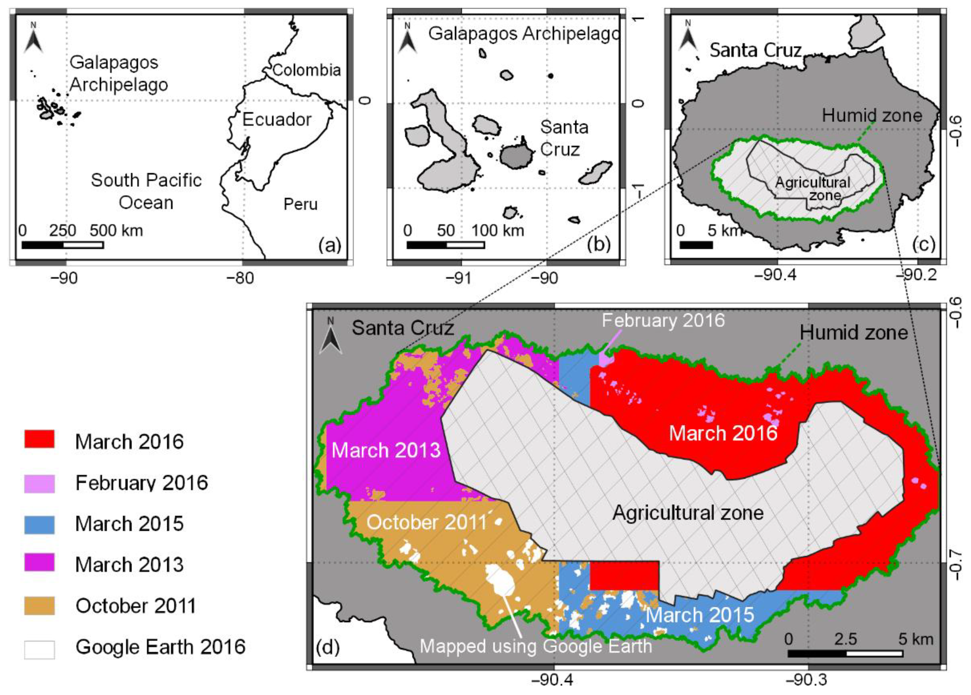
Our research was conducted in the Galapagos archipelago, a UNESCO World Heritage Site, which is known for its high endemism of species [18]. Sadly, the unique biodiversity of terrestrial ecosystems is currently under threat from invasive plant species [8,19]. To be able to prioritize management actions for these invasive species, accurate distribution maps of individual species are required. Both very-high-resolution (VHR) and medium-resolution (MR) satellite imagery have been used to map the extension of invasive and other plant species in the Galapagos Islands in the past. For example, Trueman et al. [20] used VHR imagery from the WorldView-2 imaging satellite to produce a spatial database of canopy plant densities in the protected areas of the highlands of Santa Cruz Island. The database consisted of manually delineated polygons, which included a density measure for several vegetation cover classes. Rivas-Torres et al. [21] used MR from the Landsat 8 imaging satellite to develop an object-based methodology for mapping native and invasive vegetation cover for the protected area on all islands in the archipelago, resulting in a spatial database of vegetation units at an “ecosystem scale” that included units dominated by invasive species. Laso et al. [22] mapped the agricultural zone, and a buffer surrounding this area, on the inhabited islands, using a combination of high resolution (HR) PlanetScope and MR Sentinel-2 satellite imagery.

The objective of our study was to advance this previous work by incorporating the detailed information of VHR imagery to model the distribution and abundance of dominant invasive plant species. Our goal was to show the effects that the spatial resolution of satellite imagery has on the outcomes of vegetation mapping in the highlands of Santa Cruz in the Galapagos National Park (GNP) area by comparing our maps produced with VHR imagery with maps produced with MR imagery by Rivas-Torres et al. [21]. We hypothesized that VHR imagery, apart from delivering more accurate results, was crucial for the mapping of plant species with less distinctive growth forms. We argue that whereas lower resolution could be suitable for the mapping of plant species with more distinctive growth forms, higher-resolution imagery may be indispensable for the mapping of species with less distinctive growth forms.

2. Materials and Methods

2.1. Study Area

The Galapagos archipelago is located in the Pacific Ocean, approximately 1000 km west of the South American coast on the equator (1°40′ N–1°36′ S, 89°16′–92°01′ W) (Figure 1a,b). This archipelago comprises about 123 islands, of which only about 15 count as main islands [23]. The largest islands have a climatic zonation, stretching from the dry lowlands to the humid highlands [24]. Our study area is located on Santa Cruz Island, in the humid highlands of the Galapagos National Park (GNP) (Figure 1c). The highest elevation on this island is 864 m.a.s.l., and the mean annual precipitation between 1988 and 2018 was 1059 mm at 223 m.a.s.l. (0°41′33″ S, 90°19′41″ W) [25]. Because other studies have used different boundaries for delimiting the “humid zone”, we present our delimitation method in Appendix A. The humid zone is characterized by high biological productivity and by housing many endemic species [18]. It is also the area colonized by the early settlers, who cultivated the land and introduced new plant species, many of which have become invasive [26], especially following anthropogenic fires [27]. The first sustained agricultural efforts in this area began in 1910 [28]. As other farmers arrived in subsequent decades, cultivation and livestock activities continued to increase. The Galapagos National Park (GNP) was established in 1959, and by 1974, 97% of the land area of the archipelago was protected, while the remaining 3% was assigned to human settlements and agricultural use (most of which is located in the highlands) [29].

2.2. Very-High-Resolution Species Mapping

2.2.1. Satellite Imagery

Very-high-resolution (VHR) images have a spatial resolution of 5 m or less, i.e., the pixels represent areas smaller than 5 m × 5 m on the ground [16], and a tree or plant is represented by one or a few pixels. In this study, we used VHR WorldView-2 (WV-2) images. The WV-2 sensor has a spatial resolution of 0.5 m in the panchromatic band and 2 m in the spectral bands [13,30] and is among the few VHR multispectral sensors with eight bands situated in the visible and near-infrared regions of the spectrum: Band 1, Coastal (400–450 nm); Band 2, Blue (450–510 nm); Band 3, Green (510–580 nm); Band 4, Yellow (585–625 nm); Band 5, Red (630–690 nm); Band 6, Red Edge (705–745 nm); Band 7, Near-Infrared 1 (770–895 nm); and Band 8, Near-Infrared 2 (860–1040 nm) [15].

We used mainly cloud-free (<10% cloud cover) WV-2 satellite images acquired during the hot and wet season in Galapagos, between February and March [31], for the years 2013, 2015, 2016, and, additionally, an image from the cool and dry season in October 2011 (Figure 1d). Images of the hot and wet season were preferred, since they are generally free of clouds and the vegetation is green and lush and at its maximum response level, allowing for better spectral separability between the plant species [13]. For the southwestern part of our study area, we were only able to obtain a mostly cloud-free image captured in October 2011. However, we do not think that this affected the outcome of the mapping, since the sole dominant invasive species in this area was the easily discernible Cuban cedar. Pixels covered by clouds or cloud shadows in all images were masked out by manually drawing their boundaries. The resulting gaps were then replaced by matching areas of WV-2 images from earlier dates. For example, a cloud gap from a WV-2 image from March 2016 was replaced by the WV-2 image from February 2016. Cloud gaps for which no other WV-2 image existed, as was the case for cloud-covered portions in the March 2015 and October 2011 images, were replaced with Google Earth (GE) satellite imagery from 2016 (Figure 1d). In the cloud gaps evaluated with GE satellite imagery, target species were manually delineated.

To obtain the spectral reflectance signatures of the plant species to map, the radiometrically corrected digital numbers (DNs) of the WV-2 satellite imagery were transformed to top-of-atmosphere (TOA) spectral reflectance, according to Updike and Comp [32], using the satellite package [33] in the R 3.5.0 statistical software environment [34].

2.2.2. Segmentation for Object-Based Image Analysis

Very high spatial resolutions have enough detail to distinguish individual plants in heterogeneous landscapes. However, when the pixel dimensions are smaller than the size of individual tree crowns, there is an increase in the variability of the signatures of pixels that cover the same tree [16]. Therefore, we adopted an object-based image analysis (OBIA) approach that groups spatially and spectrally close pixels into objects, representing features such as individual tree crowns, as it yields better results in species identification than classification methods based solely on the spectral properties of the pixels [9,35]. Based on pilot trials with different levels of segmentation, we used this approach with a two-level segmentation on the panchromatic band using eCognition Developer 10.0, Trimble GmbH (Munich, Germany). On the parent level, we generated object segments large enough to contain homogeneous forest stands or tree groups of approximately 0.5 to 3 ha in size. On the child level, we generated object segments approaching the size of single tree crowns or small shrub stands of approximately 100 to 500 m² in size.

2.2.3. Classification Model

To evaluate how different satellite imagery resolutions affect the mapping of plants belonging to different growth forms, we chose the following invasive plant species: (1) tall tree: Cuban cedar (Cedrela odorata), with a large crown and lush foliage with high photosynthetic activity, (2) medium tree: common guava (Psidium guajava), with an irregular crown and leaves with lower photosynthetic activity, and (3) shrub: blackberry (Rubus niveus), forming a dense understory thicket, often covered by other vegetation. Cedrela odorata was the tallest tree species in our study area at up to 20 m in height, Psidium guajava had up to 7 m in height, and Rubus niveus had up to 2 m in height. All of these species had originally been planted in the agricultural zone and have now spread into the GNP [26].

There are multiple remote sensing classification models using satellite imagery, whereby the user classifies training objects. Subsequently, an algorithm uses these data to predict unclassified objects. For the classification of our target species, we chose a Random Forest (RF) model, which is a nonparametric classification technique based on ensemble machine learning [36]. Random Forest has been deemed as the classifier of choice by several studies because of its ability to overcome overfitting limitations and to achieve the best overall accuracy results compared to other models [12,37]. We used the mean reflectance of each spectral band and the panchromatic band as our model parameters, since including all spectral dimensions in WV-2 had a greater predictive power [38]. In addition, we included the standard deviation (SD) in the panchromatic band to characterize vegetation textures, as suggested by Berhane et al. [12]. Each child-level object inherited the SD from its parent-level object. The parent-level objects were large enough to differentiate the low SD in the smooth texture of grass patches from the high SD in the rough texture of forested stands. For each WV-2 satellite image, a separate RF model was trained. The statistical software R 3.5.0 [34] and the packages caret [39], raster [40], and randomForest [41] were used for the classification.

For each object, we calculated the Normalized Difference Vegetation Index (NDVI), an index used to identify and measure live green vegetation, with values ranging from −1 to 1 [42]. Negative values indicate clouds, water, and snow; values close to zero indicate bare soil, and positive values vegetated areas. Values close to 1 indicate the highest density of green leaves. Because our target species of Cuban cedar, guava, and blackberry had an average NDVI greater than 0.6, this model was only applied to objects above this threshold. Pasture areas and tree patches of avocado (Persea americana), red quinine (Cinchona pubescens), and rose-apple (Syzygium jambos), which were visually recognizable from the satellite imagery, were manually delineated and excluded from the model to avoid spectral confusion. To better distinguish our target species from other vegetation, all main species present in the humid zone of Santa Cruz were included in the model. Because we were not only differentiating between species, but also between the different phenology stages of a species, we hereafter refer to these as “classes” and not species. Sixteen classes representing the dominant plant species visible in the study area were included: Cuban cedar, guava, blackberry, Scalesia (Scalesia pedunculata), Miconia (Miconia robinsoniana), bracken (Pteridium arachnoideum), dry bracken, glorybower (Clerodendrum molle), Croton (Croton sp.), manchineel tree (Hippomane mancinella), guayabillo (Psidium galapageium), “Cuban cedar 2” (Cuban cedar with young and bright colored leaves), “green moss” (trees with crowns dominated by green moss and liverwort epiphytes), “mixed vegetation” (patches where a single dominant species could not be defined), and “shadow” (various types of vegetation obscured by shadows). To determine the suitability of the assigned classes, we calculated their Jeffries–Matusita distance (JMD). The JMD is a spectral separability measure that can be used to quantify similarities between classes [43]. The JMD values range from 0 to 2, with values < 1 suggesting poor separability, and values closer to 2, high separability [12]. We calculated the JMD for all classes in the model generated for the WV-2 image from March 2016. We chose this image because it covered the largest area in our study area, with a high presence of all target species. After initial classification, some objects were reclassified based on a ruleset described in Appendix B.

Training and validation points were marked by the Global Positioning System or interpreted visually from orthophotos obtained from unmanned aerial vehicles, which had a spatial resolution of <6 cm. For each model, an equal number of sample points per class was assigned, so that all classes were equally represented [38]. We used 200 sample points per class, of which 140 sample points were used to train the model and 60 to validate the classifications. When a model class could not be represented by 200 points, fewer sample points were used, maintaining a 7/3 ratio between the training and validation points. If there were less than 100 sample points to represent a class, we did not include this class in the RF model of that image. This happened when a class was not present within the area covered by an image. For example, there was no Miconia within the area covered by the WV-2 image from March 2013, so this class was not included in the RF model of that image. This scenario did not come up with any of our target species. Validation points from each WV-2 satellite image were used to calculate a confusion matrix. The overall accuracy (OA), Kappa, and class sensitivities derived from these confusion matrices were used to describe the performance of their corresponding classification model. OA is the number of correctly classified points divided by the total number of validation points in each model. Kappa compares the difference between the accuracy of the model with the accuracy expected by chance [44,45]. Class sensitivity is the ratio of correct positive predictions, divided by the total number of positive predictions of each class. Finally, the weighted average of each metric was calculated. As a weighting factor, we used the area covered by each WV-2 image, divided by the study area mapped using WV-2 images.

2.3. Comparison of Very-High and Medium-Resolution Species Distribution Mapping

2.3.1. Medium-Resolution Species Distribution Resource

Pixels in MR imagery are a few tens of meters in size and each one encompasses several individual trees or plants [15]. To represent MR maps in our study area, we used the results published by Rivas-Torres et al. [21]. The authors mapped the ecosystems and invasive species in Galapagos, using multispectral Landsat 8 imagery pansharpened at 15 m spatial resolution. The main image used for Santa Cruz was captured in March 2016, and cloud-covered gaps were replaced with an image captured in February 2015. The images were segmented though OBIA and objects were classified with a fuzzy membership function. To demonstrate how spatial resolution affects the quality of the mapping results, we overlapped and compared our maps using VHR with the maps generated by Rivas-Torres et al. [21] for each target species.

2.3.2. Validation of Mapping Results

A comparison of the map accuracy for VHR and MR was performed using the OA and Kappa of a traditional confusion matrix. A total of six confusion matrices were computed, one for each target species and resolution type (MR and VHR). For each target species, we performed a Z-test between VHR and MR confusion matrices, following Moity et al. [44]. A |Z| value ≥ 1.96 indicated a statistically significant difference between the classification performed with both resolution types. Each confusion matrix was based on 100 validation points. Half of these points were placed at random in areas of predicted presence and the other half in areas of predicted absence of the target species. Validation points from areas of predicted absence were no further than 200 m away from areas of predicted presence. No point was located within the areas mapped using Google Earth imagery, areas manually delineated as pasture or avocado patches, or areas within 2 m of any of the training objects used for the VHR mapping (see Appendix C for the location of these points). All points were validated by visual interpretation of the VHR WV-2 satellite images shown in Figure 1d. Since MR maps only included units dominated by a species, we based our comparison of validation of MR and VHR results on the following considerations: (a) for MR results, a radius of 15 m around the validation point was visually interpreted to determine whether the species dominated that area or not and (b) to validate areas of predicted presence in VHR maps, validation points were located within areas where more than 50% of the area was occupied by the species in a 15 m window. Thereby, we excluded areas from the validation, which would otherwise be impossible to detect with a 15 m resolution imagery. By the same logic, only areas where 0% of the area was occupied by the species in a 15 m window were used to validate the absence of a species (see Appendix C for the delimitation of these areas).

2.3.3. Species Cover Area

For each growth form, we calculated the species cover area obtained from our VHR maps and from MR maps by Rivas-Torres et al. [21], as well as the area where both maps overlapped. To estimate the percentage of the area gained or missed using MR imagery, we divided the area mapped with MR imagery by the area mapped with VHR imagery, and subtracted it from 1. To obtain a measure for the spatial similarity between the maps produced with both resolutions, we divided the area where MR and VHR overlapped by the total area mapped with VHR and/or MR. Thus, a 0% value would indicate that the maps do not overlap and a 100% value would indicate that the maps are identical.

Additionally, for each growth form, we compared the overall area mapped with VHR and MR imagery as polygons of different sizes, ranging from ≤0.25 ha (small), >0.25 to 10 ha (medium), >10 to 50 ha (large), and >50 to 100 ha (very large). This gave us information about the contribution of smaller or larger polygons to the area estimated in both VHR and MR imagery.

3. Results

3.1. Very-High-Resolution Species Mapping

We produced five RF models generated from five WV-2 satellite images. The percentage contribution of each WV-2 image to the study area mapped with WV-2 is shown in

Table 1. Overall accuracies and Kappa obtained from confusion matrices calculated with the validation points from the Random Forest (RF) model developed for each WV-2 satellite image, as well as the sensitivity of the three target species. Weighted averages were calculated using the percentage that each image occupies in the area mapped, using WV-2 images as the weighting factor. Complete confusion matrices are included in Appendix D.

	March 2016	February 2016	March 2015	March 2013	October 2011	WeightedAverage
Overall accuracy	87%	88%	85%	85%	86%	86%
Kappa	0.86	0.87	0.83	0.83	0.84	0.85
Tall tree (Cuban cedar) sensitivity	92%	82%	96%	85%	97%	90%
Medium tree (guava) sensitivity	84%	81%	86%	67%	77%	79%
Shrub (blackberry) sensitivity	85%	77%	78%	83%	90%	86%
Percentage of the image in the study area mapped using WV-2 satellite images (Weighting factor)	41.2%	0.9%	14.2%	19.9%	23.8%

. This percentage was used as a weighting factor to calculate the weighted averages of OA (also shown in Table 1), Kappa, and class sensitivity of the three target species, derived from the confusion matrices generated with the validation points from the RF model of each WV-2 image. Complete confusion matrices are shown in Appendix D (

Table A1. Complete confusion matrices calculated with the validation points from the Random Forest (RF) models of each WorldView-2 (WV-2) image.

March 2016
		Reference
		Cuban cedar	Cuban cedar 2	Blackberry	Guava	Mixed vegetation	Bracken	Dry bracken	Croton	Scalesia	Green moss	Miconia	Glorybower	Manchineel tree	Shadow
Prediction	Cuban cedar	55	4	0	0	0	0	0	0	0	0	0	0	0	0
	Cuban cedar 2	3	54	0	0	0	0	0	0	0	0	0	0	0	0
	Blackberry	0	2	50	0	0	1	0	0	3	0	0	0	0	0
	Guava	1	0	0	48	5	0	0	0	1	0	0	0	2	0
	Mixed vegetation	0	0	0	5	39	0	3	0	0	0	1	0	2	0
	Bracken	0	0	4	0	0	55	0	1	0	0	0	0	0	0
	Dry bracken	0	0	0	0	16	0	57	0	0	0	0	0	0	0
	Croton	0	0	1	0	0	0	0	55	4	1	0	0	0	0
	Scalesia	0	0	2	2	0	1	0	2	50	6	0	0	0	0
	Green moss	0	0	1	2	0	3	0	1	1	47	0	5	16	0
	Miconia	0	0	0	0	0	0	0	0	0	0	59	0	0	0
	Glorybower	0	0	0	0	0	0	0	1	0	0	0	55	0	0
	Manchineel tree	0	0	1	0	0	0	0	0	0	6	0	0	40	0
	Shadow	1	0	0	0	0	0	0	0	1	0	0	0	0	60
	Sensitivity (%)	92	90	85	84	65	92	95	92	83	78	98	92	67	100
	Overall Accuracy (OA): 87%
	Kappa: 0.86
February 2016
		Reference
		Cuban cedar	Cuban cedar 2	Blackberry	Guava	Mixed vegetation	Bracken	Dry bracken	Croton	Scalesia	Green moss	Miconia	Glorybower	Shadow
Prediction	Cuban cedar	49	5	0	1	0	0	0	0	1	0	0	0	0
	Cuban cedar 2	7	52	4	0	0	0	0	0	0	0	0	0	0
	Blackberry	0	3	46	0	0	9	0	1	2	0	0	0	0
	Guava	1	0	0	48	8	2	0	0	6	1	0	0	2
	Mixed vegetation	2	0	3	7	52	3	0	0	1	0	1	0	2
	Bracken	0	0	7	0	0	42	1	1	2	1	0	0	0
	Dry bracken	0	0	0	1	0	0	58	0	0	0	0	0	0
	Croton	0	0	0	0	0	0	0	52	0	0	0	0	0
	Scalesia	0	0	0	0	0	2	0	1	47	1	0	0	0
	Green moss	1	0	0	2	0	0	0	0	0	57	0	5	16
	Miconia	0	0	0	0	0	0	1	0	0	0	59	0	0
	Glorybower	0	0	0	0	0	2	0	1	1	0	0	95	0
	Shadow	0	0	0	0	0	0	0	0	0	0	0	0	40
	Sensitivity (%)	82	87	77	81	87	70	97	93	78	95	98	92	67
	Overall Accuracy (OA): 88%
	Kappa: 0.87
March 2015
		Reference
		Cuban cedar	Cuban cedar 2	Blackberry	Guava	Mixed vegetation	Bracken	Dry bracken	Croton	Scalesia	Green moss	Miconia	Glorybower	Shadow
Prediction	Cuban cedar	50	4	0	0	1	0	0	0	0	0	0	0	0
	Cuban cedar 2	3	44	4	0	1	0	0	0	3	0	0	1	0
	Blackberry	1	7	47	0	0	9	0	0	5	0	0	0	0
	Guava	2	0	0	51	11	0	0	0	0	0	0	0	0
	Mixed vegetation	1	2	0	6	41	0	1	0	0	0	0	2	1
	Bracken	0	1	5	0	1	47	0	0	1	0	0	0	0
	Dry bracken	0	0	2	0	1	1	56	2	0	0	2	0	0
	Croton	0	0	0	0	0	0	0	51	0	0	0	3	1
	Scalesia	0	0	1	0	0	1	0	0	44	2	0	0	0
	Green moss	2	1	1	2	1	2	1	0	6	58	0	0	0
	Miconia	0	0	0	0	0	0	1	0	0	0	49	1	0
	Glorybower	0	1	0	0	2	0	1	5	0	0	0	53	0
	Shadow	1	0	0	0	1	0	0	0	0	0	0	0	55
	Sensitivity (%)	83	73	78	86	68	78	93	88	75	97	96	88	96
	Overall Accuracy (OA): 85%
	Kappa: 0.83
March 2013
		Reference
		Cuban cedar	Cuban cedar 2	Undefined	Blackberry	Guava	Mixed vegetation	Croton	Scalesia	Green moss	Guayabillo	Glorybower	Shadow
Prediction	Cuban cedar	51	5	1	0	0	0	0	0	0	0	0	0
	Cuban cedar 2	7	55	0	0	0	0	0	1	0	0	2	0
	Undefined	2	0	55	0	0	2	0	1	2	0	0	1
	Blackberry	0	0	0	10	0	0	0	2	0	0	2	0
	Guava	0	0	0	0	12	0	0	1	0	3	1	0
	Mixed vegetation	0	0	4	0	1	48	0	0	3	1	0	0
	Croton	0	0	0	0	1	0	53	6	1	0	2	0
	Scalesia	0	0	0	0	0	1	0	19	1	0	0	0
	Green moss	0	0	0	0	1	1	0	5	47	0	0	0
	Guayabillo	0	0	0	0	3	8	0	2	0	56	3	0
	Glorybower	0	0	0	0	0	0	0	5	1	0	50	0
	Shadow	0	0	0	0	0	0	0	0	0	0	0	54
	Sensitivity (%)	85	92	92	83	67	80	88	45	84	93	83	98
	Overall Accuracy (OA): 85%
	Kappa: 0.83
October 2011
		Reference
		Cuban cedar	Blackberry	Guava	Mixed vegetation	Bracken	Dry bracken	Croton	Scalesia	Green moss	Miconia	Glorybower	Shadow
Prediction	Cuban cedar	58	0	0	0	1	0	0	0	0	0	0	0
	Blackberry	0	54	0	0	2	0	0	8	2	0	0	0
	Guava	0	0	44	14	0	0	0	0	0	1	2	0
	Mixed vegetation	1	0	10	43	1	0	0	0	0	0	4	1
	Bracken	0	0	0	0	17	0	0	0	0	0	0	0
	Dry bracken	0	0	0	0	0	41	0	0	0	0	0	0
	Croton	0	0	0	0	0	0	58	1	0	0	0	0
	Scalesia	0	1	0	0	0	0	0	46	10	0	0	0
	Green moss	0	1	1	3	2	0	1	4	47	0	0	0
	Miconia	0	0	0	0	0	0	0	0	0	57	0	0
	Glorybower	0	4	1	0	0	1	1	3	1	0	3	0
	Shadow	1	0	1	0	0	0	0	0	0	0	4	59
	Sensitivity (%)	97	90	77	72	74	98	97	74	78	98	23	98
	Overall Accuracy (86%)
	Kappa 0.84

). The resulting OAs ranged from 85% to 87% (86% weighted average), and their corresponding Kappa ranged from 0.83 to 0.86 (0.85 weighted average). The class sensitivity of our target species was highest for the tall tree growth form (Cuban cedar), ranging from 83% to 97% (90% weighted average), intermediate for the shrub growth form (blackberry), ranging from 77% to 90% (86% weighted average), and lowest for the medium tree growth form (guava), ranging from 67% to 86% (79% weighted average). Raster files of the maps produced with VHR imagery can be found in the Supplementary Materials section.

The similarity between the model classes can be observed from the Jeffries–Matusita distance (JMD) values shown in

Table 2. Jeffries–Matusita distance (JMD) table calculated from the spectral values of the training samples taken from WV-2 image captured in March 2016. JMDs involving guayabillo were derived from a JMD table calculated from the March 2013 WV-2 image, because the guayabillo samples were not sufficiently represented in the March 2016 image.

	Cuban cedar	Cuban cedar 2	Blackberry	Guava	Mixed vegetation	Bracken	Glorybower	Guayabillo	Scalesia	Green moss	Miconia	Manchineel tree	Dry bracken	Croton	Shadow
Cuban cedar
Cuban cedar 2	1.35
Blackberry	1.41	1.40
Guava	1.41	1.41	1.41
Mixed vegetation	1.41	1.41	1.41	1.38
Bracken	1.41	1.41	1.33	1.41	1.40
Glorybower	1.41	1.41	1.41	1.41	1.41	1.41
Guayabillo	1.41	1.41	1.41	1.40	1.28	1.40	1.40
Scalesia	1.41	1.41	1.39	1.40	1.41	1.41	1.41	1.38
Green moss	1.41	1.41	1.40	1.40	1.41	1.41	1.40	1.40	1.37
Miconia	1.41	1.41	1.41	1.41	1.41	1.41	1.41	1.41	1.41	1.41
Manchineel tree	1.41	1.41	1.41	1.41	1.41	1.41	1.41	1.41	1.41	1.39	1.41
Dry bracken	1.41	1.41	1.41	1.41	1.35	1.41	1.41	1.41	1.41	1.41	1.41	1.41
Croton	1.41	1.41	1.41	1.41	1.41	1.41	1.41	1.40	1.41	1.40	1.41	1.41	1.41
Shadow	1.41	1.41	1.41	1.41	1.41	1.41	1.41	1.41	1.41	1.41	1.41	1.41	1.41	1.41

Cuban cedar 2: Cuban cedar with young leaves. Dark gray: classes with lower separability, including at least one of the target species. Light gray: classes with lower separability, including none of the target species.

. This table was generated based on the training points from the WV-2 March 2016 satellite image, which was used to evaluate the similarity between the model’s classes, because it covered the largest percentage of the study area. The results indicated that no class combination had poor separability, as all JMD values were between 1 and 2. The highest separability measure was 1.41, with 81% of all possible class combinations reaching this value. The remaining 19% ranged from 1.28 to 1.40. Only half of those class combinations involved at least one of our target species, which were: guava and mixed vegetation, guava and Scalesia, guava and green moss, blackberry, and Cuban cedar 2, blackberry and Scalesia, blackberry and green moss, and blackberry and bracken. This last pair had the lowest separability among these class combinations.

The mean NDVI values calculated from training points in the WV-2 March 2016 satellite image ranged from 0.68 to 0.85. The values were 0.86 for Cuban cedar 2, 0.85 for Cuban cedar, 0.79 for blackberry, 0.77 for bracken, 0.77 for glorybower, 0.77 for guayabillo, 0.76 for Scalesia, 0.75 for guava, 0.75 for Miconia, 0.73 for manchineel tree, 0.72 for Croton, 0.70 for shadow, and 0.68 for mixed vegetation.

3.2. Comparison of Very-High and Medium-Resolution Species Distribution Mapping

3.2.1. Comparison of Species Distribution Maps

The maps in Figure 2a–c show the distribution of the target species mapped with either VHR or MR or both. The maps for tall tree (Cuban cedar) (Figure 2a) exhibit a large and easily discernible area where both VHR and MR maps overlap. In the maps for medium tree (guava) (Figure 2b) and shrub (blackberry) (Figure 2c), the overlap between VHR and MR is only discernible in zoom insets.

3.2.2. Comparison of Validation Confusion Matrices

The confusion matrices calculated for each target species and imagery resolution produced consistently better results for maps generated with VHR imagery than with MR imagery, with higher OA and Kappa estimates (

Table 3. Very-high-resolution (VHR) and medium-resolution (MR) confusion matrix obtained for the tall tree growth form (Cuban cedar).

Very High Resolution					Medium Resolution
Prediction		Reference			Prediction		Reference
		Presence	Absence				Presence	Absence
	Presence	47	5			Presence	45	14
	Absence	3	45			Absence	5	36
Overall accuracy (OA): 92%						Overall accuracy (OA): 81%
Kappa: 0.84						Kappa: 0.62
|Z| value: 2.28 (≥ 1.96: Statistically significant difference at p < 0.05)

,

Table 4. Very-high-resolution (VHR) and medium-resolution (MR) confusion matrix obtained for the medium tree growth form (guava).

Very High Resolution					Medium Resolution
Prediction		Reference			Prediction		Reference
		Presence	Absence				Presence	Absence
	Presence	32	6			Presence	8	11
	Absence	18	44			Absence	42	39
Overall accuracy (OA): 76%					Overall accuracy (OA): 47%
Kappa: 0.52					Kappa: −0.06
|Z| value: 4.21 (≥ 1.96: Statistically significant difference at p < 0.05)

and

Table 5. Very-high-resolution (VHR) and medium-resolution (MR) confusion matrix obtained for the shrub growth form (blackberry).

Very High Resolution					Medium Resolution
Prediction		Reference			Prediction		Reference
		Presence	Absence				Presence	Absence
	Presence	37	5			Presence	25	12
	Absence	13	45			Absence	25	38
Overall accuracy (OA): 82%					Overall accuracy (OA): 63%
Kappa: 0.64					Kappa: 0.26
|Z| value: 3.01 (≥ 1.96: Statistically significant difference at p < 0.05)

). For each target species, a comparison between the VHR and MR confusion matrices showed statistically significant differences at p < 0.05, with |Z| values ≥ 1.96 (Table 3, Table 4 and Table 5). This is an indication that the VHR maps were significantly more accurate than the MR maps. In the VHR and MR maps, the highest OA corresponded to tall tree (Cuban cedar) (92% VHR, 81% MR), the lowest OA corresponded to medium tree (guava) (76% VHR, 47% MR), and an intermediate OA corresponded to shrub (blackberry) (82% VHR, 63% MR). The percentage difference in the OA of the models produced with VHR and MR was 29% for medium tree (guava), 19% for shrub (blackberry), and 11% for tall tree (Cuban cedar). All Kappa estimates were > 0.5 in VHR, yet for MR only tall tree (Cuban cedar) presented a Kappa > 0.5. For shrub (blackberry), the Kappa was only 0.25 and for medium tree (guava), it reached a negative value.

3.2.3. Species Cover Area

To obtain the cover area of each target species (

Table 6. Area (ha) modeled for tall tree (Cuban cedar), medium tree (guava), and shrub (blackberry) growth forms, using very-high-resolution (VHR) and medium-resolution (MR) satellite imagery.

		Tall Tree (Cuban Cedar)	Medium Tree (Guava)	Shrub (Blackberry)
Area modeled with VHR		1812.2	855.0	283.0
Area modeled with MR		1687.7	546.8	127.3
Percentage difference of area estimated with MR, divided by area estimated with VHR		6.9%	36.8%	55.0%
Area of overlap between VHR and MR		1193.1	29.3	15.9
Total area modeled with VHR and/or MR		2306.8	1372.4	394.4
Percentage of area of overlap between VHR and MR, divided by the area mapped with VHR and/or MR		51.7%	2.1%	4.0%

), we used the maps shown in Figure 2. The areas modeled with VHR were consistently larger than those modeled with MR. For both resolutions, the largest area was covered by tall tree (Cuban cedar), an intermediate area by medium tree (guava), and the smallest area by shrub (blackberry). The more/less the areas of VHR and MR overlap, the higher/lower were the percentages of “spatial coincidence”. Tall tree (Cuban cedar) had the highest percentage of spatial coincidence area between VHR and MR (52%), divided by the area mapped with either VHR or MR or both. For medium tree (guava) and shrub (blackberry), the spatial coincidence area was smaller than 5%.

Additionally, Figure 3 shows the comparisons of the overall area mapped for each growth form for both resolutions, using different size polygons. With the medium (>0.25 to 10 ha) and large (>10 to 50 ha) polygons, the overall areas mapped for both resolutions were relatively similar. However, with the small (≤0.25 ha) and very large (>50 ha) polygons, the differences in the areas mapped with both resolutions increased. MR mapping did not consider small polygons (≤0.25 ha), while using VHR mapping, these polygons contributed 220 to 555 ha to the overall area. These polygons represented more than 60% of the overall area mapped for the medium tree (guava) and shrub (blackberry) growth forms. In contrast, with very large polygons (>50 ha), 196 ha of medium tree (guava) growth forms were mapped using MR imagery and none using VHR imagery. Similarly, 1247 ha of tall tree (Cuban cedar) growth forms were mapped using MR, compared to 146 ha using VHR imagery, which represents an increase of 213 ha (14%).

4. Discussion

Our study compared the outcome of mapping performed with very-high-resolution (VHR) and medium-resolution (MR) satellite imagery. We mapped three invasive plant species with different growth forms on Santa Cruz Island, Galapagos: tall tree, medium tree, and shrub. As expected, we found that for each growth form, VHR imagery produced models with significantly higher overall accuracy (OA) and Kappa estimates than those resulting from the models produced with MR imagery. Several studies have compared the effects of spatial resolution on the mapping of land cover classes or individual species. Müllernová et al. [46] demonstrated that higher-resolution imagery detected Heracleum mantegazzianum (giant hogweed) plants more reliably. Another study from the Interior Atlantic Forest in Paraguay found that satellite imagery of higher resolution delineated land cover classes better and identified smaller patches with greater accuracy [17]. 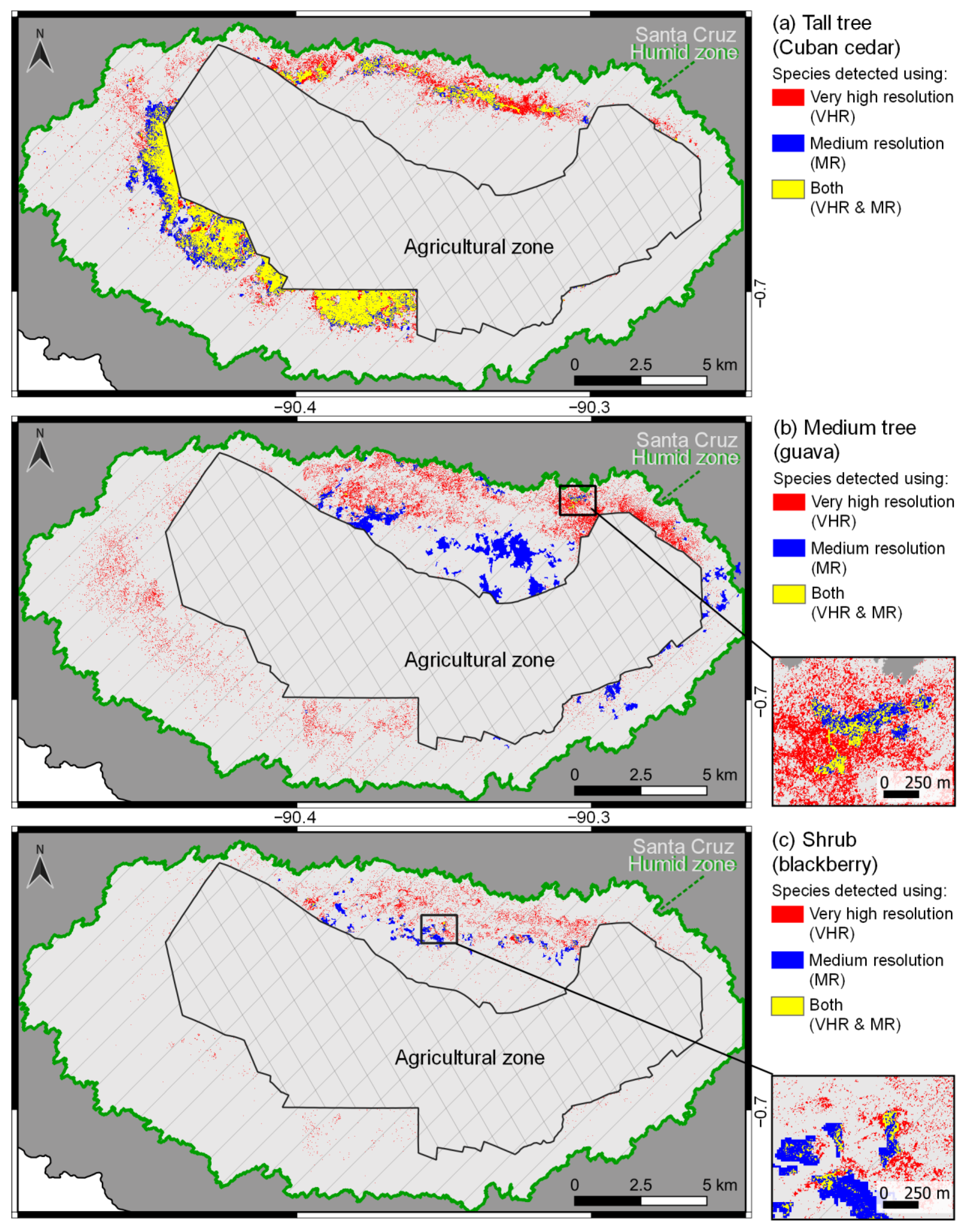A study from south-eastern Brazil showed that higher spatial resolution was better at detecting land cover classes and estimating the total load of suspended solids in water bodies [47]. What is novel about our study is that we carried out a comparison of the mapping results using VHR and MR imagery across an array of different growth forms. We showed that the map resulting from MR imagery of the tall tree growth form (Cuban cedar) was moderately similar to the one resulting from VHR imagery. However, we also found that for the medium tree (guava) and shrub (blackberry) growth forms, the maps based on MR imagery widely diverged from those produced with VHR imagery.

A model performance comparison for each growth form and resolution revealed the best OA results for the tall tree growth form (Cuban cedar) (92% VHR, 81% MR), followed by the shrub (blackberry) (82% VHR, 63% MR) and the medium tree (guava) (76% VHR, 47% MR) growth forms. The weighted average of class sensitivities produced with VHR imagery was also highest for the tall tree growth form (Cuban cedar) (90%), followed by the shrub (blackberry) (86%) and the medium tree (guava) (79%) growth forms. Kappa estimates ≥ 0.5 were obtained for all VHR models and for the MR model for the tall tree growth form (Cuban cedar) only. The Kappa estimates showed that these models had a likelihood of accuracy ≥ 50% better than expected by chance alone [45], thus indicating the models’ suitability. The highest Kappa estimate was obtained for the VHR maps of the tall tree growth form (Cuban cedar) (0.84), followed by the VHR maps of the shrub growth form (blackberry) (0.64), the MR maps of the tall tree growth form (Cuban cedar) (0.62), and the VHR maps of the medium tree growth form (guava) (0.52). While the MR model for the tall tree growth form (Cuban cedar) did not perform as well as the VHR model, its Kappa estimate showed that it still performed ≥ 50% better than by chance alone. Moreover, the OA for this MR model was only 11% lower than that for the VHR model (Table 3). In contrast, the OA for the shrub (blackberry) model based on MR imagery was 19% lower than the one based on VHR imagery (Table 5). The OA for the medium tree (guava) model based on MR imagery was as much as 29% lower than the one based on VHR imagery (Table 4). Furthermore, the Kappa estimates revealed the unsuitability of MR imagery for mapping the medium tree (guava) and the shrub (blackberry) growth forms. The VHR and MR maps of these last two growth forms occupied different spatial distributions, with an overlap of as little as 2.1% of the total area mapped with VHR and/or MR.

The diverging spatial distributions for the medium tree (guava) and shrub (blackberry) growth forms in maps produced with VHR and MR imagery (Figure 2b,c), and the low Kappa estimates (<0.5) for these MR models (Table 4 and Table 5), showed that the MR area estimates were unreliable. Reliable estimates of the area covered by invasive species are crucial to help assess the extent of an invasion and to plan the resources needed to control these species [48,49]. However, while higher resolutions usually provide the most accurate estimates, there are cases where lower resolutions can deliver comparable results. For example, when comparing forest cover in eastern Paraguay, only marginal differences were encountered between the MR and VHR total area estimates [17]. We found a similar result when mapping the tall tree growth form (Cuban cedar) produced by MR, which underestimated the area by only 6.9% (Table 6). The comparability of MR and VHR maps for the tall tree growth form is further evidenced by the similar spatial distribution of both maps and the ≥0.5 Kappa estimates in the models produced with both resolutions (Table 3).

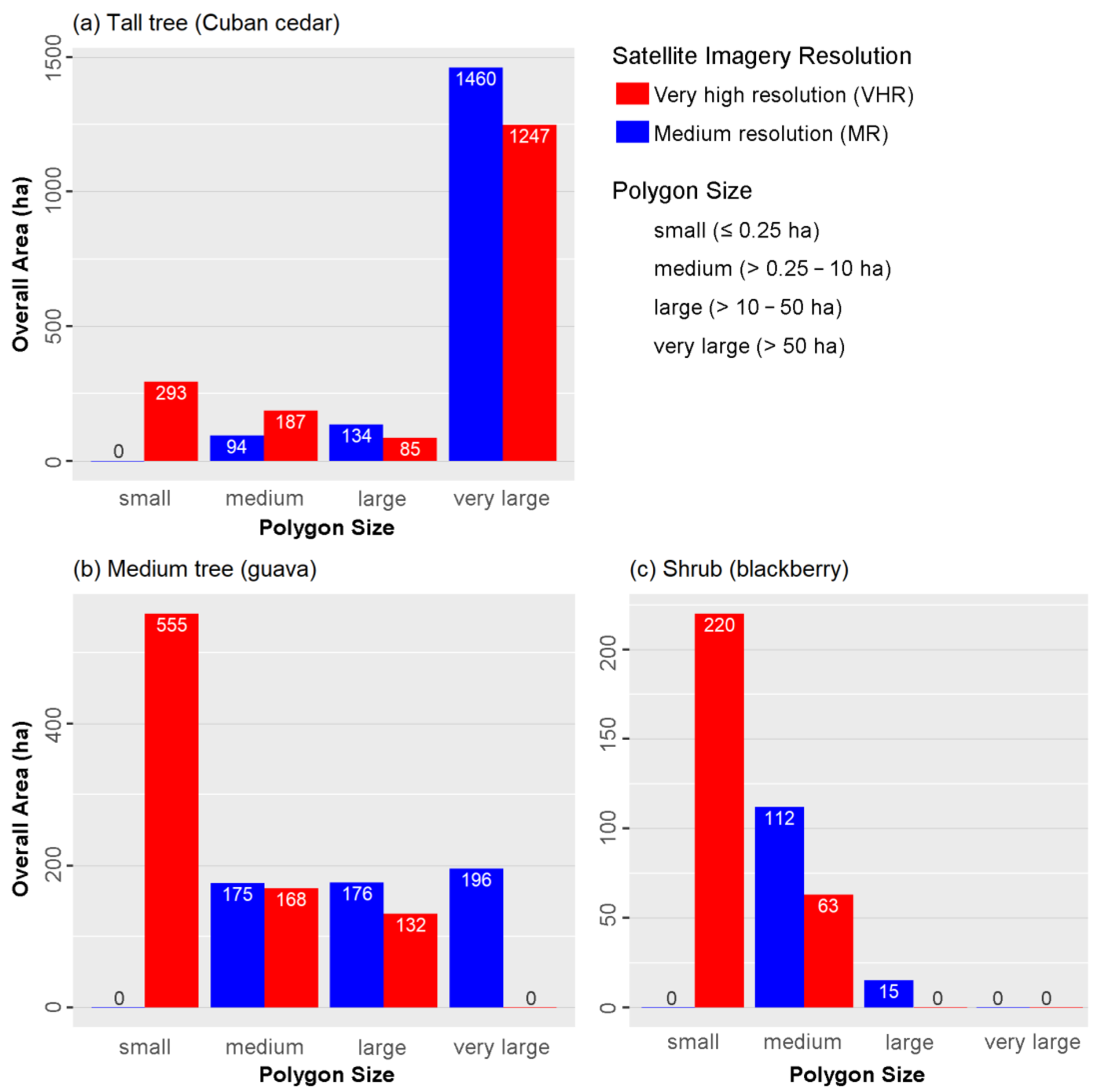
The similarity between the maps of the tall tree growth form (Cuban cedar) produced by VHR and MR (Figure 2a) was probably due to the fact that most of the space occupied by Cuban cedar consisted of large monospecific stands, which were primarily detected with very large polygons. Only a minor portion was detected with the small polygons exclusively present in VHR maps (Figure 3a). The high accuracy in detecting the tall tree growth form (Cuban cedar) with MR imagery can be explained by the distinctiveness of this plant species from others. Cuban cedar was the tallest tree in our study area, had the largest crown, and was hardly ever shaded by other vegetation. During the wet season, the crowns were lush green, resulting in a high photosynthetic activity and a mean NDVI of 0.85, the highest among the classes analyzed. The high JMD also evidenced the distinctiveness of Cuban cedar compared to all other classes.

The spatial distributions of the medium tree (guava) and the shrub (blackberry) growth forms were more scattered (Figure 2b,c). Most of their overall area was detected by small polygons (≤0.25 ha) with VHR imagery, but not with MR imagery (Figure 3b,c). Similar results were encountered for the mangrove mapping in Galapagos, where MR mapping was unable to detect 60% of the mangrove distribution because 85% of the mangrove patches were smaller than 0.5 ha [44]. These results highlight the need to use VHR imagery to map small vegetation patches. This is particularly crucial at the early stages of plant invasions, when effective control or even eradication might still be possible [50,51].

The medium tree growth form (guava) was the most difficult to discern from other vegetation and its OA was the lowest of the growth forms for both resolutions (76% VHR, 47% MR). We believe that this was due to the difficulty in differentiating guava from other classes in the study area. Indices such as the Normalized Difference Vegetation Index (NDVI) have been used for coarse differentiation between native and non-native vegetation [21,52]. However, the mean NDVI obtained for guava in our study was relatively low and similar to other vegetation types, so a clear separation was impossible. Jeffries–Matusita distance (JMD) values for guava, mixed vegetation, Scalesia, guayabillo, and green moss were very low and confirmed the spectral similarity between these classes.

Modeling the distribution of the shrub growth form (blackberry) proved to be challenging because much of the blackberry was hidden in the understory and only visible at the top layer of vegetation as small patches. Additionally, blackberry has a spectral similarity to the native bracken (Pteridium arachnoideum), which makes separating both species difficult. Additional drone footage could be used to help distinguish the two classes and to further improve the model.

Other studies also show that VHR outperforms MR in land cover classification, achieving higher OA and detection of small units [17,44,53]. Satellite imagery with lower spatial resolution is dominated by pixels that present a mixed signature average across multiple objects and, therefore, it is typically used to study ecological systems and map broad vegetation communities from regional to landscape scales [15,16]. At a higher spatial resolution, individual objects, such as tree crowns or small patches of plants, are recognizable [15,54] and, therefore, it is the preferred resolution for classifying individual species such as invasive species, or for biodiversity assessments in general [9,14,15]. However, using MR to classify invasive species can be a cost-effective way to provide an overview of areas dominated by these species [21].

Multispectral VHR imagery is not free to use and the costs can be unaffordable when management resources are scarce [55,56]. Multispectral MR imagery with global coverage is currently available at no cost, thanks to programs such as the joint NASA/USGS Landsat and the European Space Agency Sentinel. Therefore, MR imagery is an asset for low- to middle-income, but highly biodiverse countries such as Ecuador. Multispectral VHR imagery can also be prohibitive in terms of the increased computer power needed to analyze this type of imagery compared to MR, increasing the cost of the analysis [46,57]. Cost is an important factor when choosing the source resolution for mapping. Hopefully, with increasing technological advances, VHR programs will eventually provide free access to their imagery databases for academia and conservation.

One potential limitation of our study is that differences in the mapping results encountered could also have been caused by other factors besides spatial resolution, such as different acquisition dates of the imagery or the classification methods used. However, the acquisition dates for the MR and VHR imagery were very similar for most of the study area. The classification methods used with VHR imagery were similar to those used with MR imagery in that both used an object-based image analysis approach. However, they were different in the statistical classification method applied and in the segmentation methodology. For example, the segmentation methodology applied on VHR imagery produced segments that represented single trees, which would not be a discernable segment unit in MR. While we compared the results obtained with slightly different classification methods, we argue that classification methods are not always directly transferable across spatial resolutions. Therefore, we believe that a comparison of the results obtained with the methodology best suited for each resolution is still very relevant for understanding the strengths and limitations of different spatial resolutions in the mapping of different plant growth forms.

Future studies on the effects of using different spatial resolutions will improve our understanding of the outcomes of vegetation mapping, as will the exploration of different classification methods. Given the promising results obtained in this study, we recommend testing the ability of VHR imagery to detect other important plant species with similar growth forms in Galapagos and expanding the mapping to the rest of the islands in the archipelago, as well as to similar ecosystems around the world.

5. Conclusions

Our study suggests that MR can be a suitable resource to map the distribution of plant species with growth forms that contrast well with their environment and form large monospecific stands, such as the tall Cuban cedar tree. However, for other plant species with smaller growth forms that contrast less with their environment, MR imagery did not provide reliable results. Despite the fact that MR imagery is more accessible, we recommend the use of VHR imagery in the case of problematic invasive species that are difficult to distinguish from other species, such as guava and blackberry.

The VHR maps resulting from this study did not only show the distribution of the invasive species, but also their abundance. This feature is essential to prioritize management actions to control these invaders, especially when funds to do so are scarce. If management decisions were based on inaccurate maps, control costs could exceed VHR mapping costs in the long run, thus minimizing overall management success [17,58]. As plant invasions are rapidly changing due to dynamic processes such as often relatively rapid changes in species distribution and abundance [59], the results from this study also provided a baseline for tracking the spread of invasive species over time. In addition, they help identify cases where species of a certain growth form can be mapped using more accessible lower-resolution imagery. Finally, the results of this study can be applied to other parts of the world, where invasive plant species are plentiful and management decisions have to be chosen wisely [60].

References

1. Early, R.; Bradley, B.A.; Dukes, J.S.; Lawler, J.J.; Olden, J.D.; Blumenthal, D.M.; Gonzalez, P.; Grosholz, E.D.; Ibañez, I.; Miller, L.; et al. Global threats from invasive alien species in the twenty-first century and national response capacities. Nat. Commun. 2016, 7, 12485. [Google Scholar] [CrossRef] [PubMed] [Green Version]
2. Barbosa, J.M.; Asner, G.P.; Martin, R.E.; Baldeck, C.A.; Hughes, F.; Johnson, T. Determining subcanopy Psidium cattleianum invasion in Hawaiian forests using imaging spectroscopy. Remote Sens. 2016, 8, 33. [Google Scholar] [CrossRef] [Green Version]
3. Watson, J.E.M.; Evans, T.; Venter, O.; Williams, B.; Tulloch, A.; Stewart, C.; Thompson, I.; Ray, J.C.; Murray, K.; Salazar, A.; et al. The exceptional value of intact forest ecosystems. Nat. Ecol. Evol. 2018, 2, 599–610. [Google Scholar] [CrossRef] [PubMed]
4. Pimentel, D.; Zuniga, R.; Morrison, D. Update on the environmental and economic costs associated with alien-invasive species in the United States. Ecol. Econ. 2005, 52, 273–288. [Google Scholar] [CrossRef]
5. Xu, H.; Ding, H.; Li, M.; Qiang, S.; Guo, J.; Han, Z.; Huang, Z.; Sun, H.; Zhengmin, H.; Wu, H.; et al. The distribution and economic losses of alien species invasion to China. Biol. Invasions 2006, 8, 1495–1500. [Google Scholar] [CrossRef]
6. Ballesteros-Mejia, L.; Angulo, E.; Diagne, C.; Cooke, B.; Nunez, M.A.; Courchamp, F. Economic costs of biological invasions in Ecuador: The importance of the Galapagos Islands. NeoBiota 2021, 67, 375–400. [Google Scholar] [CrossRef]
7. Macfarlane, W.W.; McGinty, C.M.; Laub, B.G.; Gifford, S.J. High-resolution riparian vegetation mapping to prioritize conservation and restoration in an impaired desert river. Restor. Ecol. 2017, 25, 333–341. [Google Scholar] [CrossRef]
8. Rentería, J.L.; Gardener, M.R.; Panetta, F.D.; Atkinson, R.; Crawley, M.J. Possible Impacts of the Invasive Plant Rubus niveus on the Native Vegetation of the Scalesia Forest in the Galapagos Islands. PLoS ONE 2012, 7, e48106. [Google Scholar] [CrossRef] [Green Version]
9. Alvarez-Taboada, F.; Paredes, C.; Julián-Pelaz, J. Mapping of the Invasive Species Hakea sericea Using Unmanned Aerial Vehicle (UAV) and WorldView-2 Imagery and an Object-Oriented Approach. Remote Sens. 2017, 9, 913. [Google Scholar] [CrossRef] [Green Version]
10. Roura-Pascual, N.; Richardson, D.M.; Krug, R.M.; Brown, A.; Chapman, R.A.; Forsyth, G.G.; Le Maitre, D.C.; Robertson, M.P.; Stafford, L.; Van Wilgen, B.W.; et al. Ecology and management of alien plant invasions in South African fynbos: Accommodating key complexities in objective decision making. Biol. Conserv. 2009, 142, 1595–1604. [Google Scholar] [CrossRef]
11. Franklin, S.E. Remote Sensing for Biodiversity and Wildlife Management; McGraw-Hill: New York, NY, USA, 2010. [Google Scholar]
12. Berhane, T.M.; Lane, C.R.; Wu, Q.; Autrey, B.C.; Anenkhonov, O.A.; Chepinoga, V.V.; Liu, H. Decision-tree, rule-based, and random forest classification of high-resolution multispectral imagery for wetland mapping and inventory. Remote Sens. 2018, 10, 580. [Google Scholar] [CrossRef] [PubMed] [Green Version]
13. Wendelberger, K.S.; Gann, D.; Richards, J.H. Using Bi-Seasonal WorldView-2 Multi-Spectral Data and Supervised Random Forest Classification to Map Coastal Plant Communities in Everglades National Park. Sensors 2018, 18, 829. [Google Scholar] [CrossRef] [PubMed] [Green Version]
14. Immitzer, M.; Atzberger, C.; Koukal, T. Tree Species Classification with Random Forest Using Very High Spatial Resolution 8-Band WorldView-2 Satellite Data. Remote Sens. 2012, 4, 2661–2693. [Google Scholar] [CrossRef] [Green Version]
15. Madonsela, S.; Cho, M.A.; Mathieu, R.; Mutanga, O.; Ramoelo, A.; Kaszta, Ż.; Van De Kerchove, R.; Wolff, E. Multi-phenology WorldView-2 imagery improves remote sensing of savannah tree species. Int. J. Appl. Earth Obs. Geoinf. 2017, 58, 65–73. [Google Scholar] [CrossRef] [Green Version]
16. Nagendra, H.; Rocchini, D. High resolution satellite imagery for tropical biodiversity studies: The devil is in the detail. Biodivers. Conserv. 2008, 17, 3431–3442. [Google Scholar] [CrossRef]
17. Boyle, S.A.; Kennedy, C.M.; Torres, J.; Colman, K.; Pérez-Estigarribia, P.E.; De La Sancha, N.U. High-resolution satellite imagery is an important yet underutilized resource in conservation biology. PLoS ONE 2014, 9, e86908. [Google Scholar] [CrossRef]
18. Snell, H.L.; Tye, A.; Causton, C.E.; Bensted-Smith, R. Current status of and threats to the terrestrial biodiversity of Galapagos. In A Biodiversity Vision for the Galápagos Islands; Charles Darwin Foundation & World Wildlife Fund: Puerto Ayora, Galapagos, Ecuador, 2002; pp. 30–47. [Google Scholar]
19. Jäger, H. Biology and Impacts of Pacific Island Invasive Species. 11. Cinchona pubescens (Red Quinine Tree) (Rubiaceae). Pac. Sci. 2015, 69, 133–153. [Google Scholar] [CrossRef]
20. Trueman, M.; Standish, R.; Orellana, D.; Cabrera, W. Mapping the extent and spread of multiple plant invasions can help prioritise management in Galapagos National Park. NeoBiota 2014, 23, 1–16. [Google Scholar] [CrossRef]
21. Rivas-Torres, G.F.; Benítez, F.L.; Rueda, D.; Sevilla, C.; Mena, C.F. A methodology for mapping native and invasive vegetation coverage in archipelagos: An example from the Galápagos Islands. Prog. Phys. Geogr. 2018, 42, 83–111. [Google Scholar] [CrossRef] [Green Version]
22. Laso, F.J.; Benitez, L.; Rivas-Torres, G.; Sampedro, C.; Arce-Nazario, J. Land Cover Classification of Complex Agroecosystems in the Non-Protected Highlands of the Galapagos Islands. Remote Sens. 2019, 12, 65. [Google Scholar] [CrossRef]
23. Snell, H.M.; Stone, P.A.; Snell, H.L. A summary of geographical characteristics of the Galapagos Islands. J. Biogeogr. 1996, 23, 619–624. [Google Scholar] [CrossRef]
24. Itow, S. Zonation Pattern, Succession Process and Invasion by Aliens in Species-poor Insular Vegetation of the Galápagos Islands. Glob. Environ. Res. 2003, 7, 39–58. [Google Scholar]
25. Charles Darwin Foundation. Climatology Database. 2021. Available online: https://www.darwinfoundation.org/en/datazone/climate/bellavista (accessed on 1 February 2021).
26. Rentería, J.; Buddenhagen, C. Invasive plants in the Scalesia pedunculata forest at Los Gemelos, Santa Cruz, Galápagos. Galapagos Res. 2006, 31, 31–35. [Google Scholar]
27. Watson, J.; Trueman, M.; Tufet, M.; Henderson, S.; Atkinson, R. Mapping terrestrial anthropogenic degradation on the inhabited islands of the Galapagos Archipelago. Oryx 2010, 44, 79–82. [Google Scholar] [CrossRef] [Green Version]
28. Maldonado, R.; Llerena, E. Historia Humana. Isla Santa Cruz; Dirección del Parque Nacional Galápagos: Puerto Ayora, Galápagos, Ecuador, 2019; pp. 31–32. [Google Scholar]
29. Amador, E.; Bliemsrieder, M.; Cayot, L.; Cifuentes, M.; Cruz, E.; Cruz, F.; Ayora, P. Plan de Manejo del Parque Nacional Galapágos; INEFAN, Ed.; Servicio Parque Nacional Galápagos, Instituto Ecuatoriano Forestal y de Áreas Naturales y Vida Silvestre: Puerto Ayora, Galapagos, Ecuador, 1996; pp. 5–6. [Google Scholar]
30. Rapinel, S.; Clément, B.; Magnanon, S.; Sellin, V.; Hubert-Moy, L. Identification and mapping of natural vegetation on a coastal site using a Worldview-2 satellite image. J. Environ. Manag. 2014, 144, 236–246. [Google Scholar] [CrossRef] [Green Version]
31. Trueman, M.; D’Ozouville, N. Characterizing the Galapagos terrestrial climate in the face of global climate change. Galapagos Res. 2010, 67, 26–37. [Google Scholar]
32. Updike, T.; Comp, C. Radiometric Use of WorldView-2 Imagery. Technical Note. 2010. Available online: https://dg-cms-uploads-production.s3.amazonaws.com/uploads/document/file/104/Radiometric_Use_of_WorldView-2_Imagery.pdf (accessed on 1 October 2020).
33. Nauss, T.; Meyer, H.; Detsch, F.; Appelhans, T. Satellite: Handling and Manipulating Remote Sensing Data. R-Package 2019. Available online: https://cran.r-project.org/web/packages/satellite/ (accessed on 1 October 2020).
34. R Core Team. R: A Language and Environment for Statistical Computing; R Core Team: Vienna, Austria, 2018; Available online: https://www.r-project.org/ (accessed on 1 October 2020).
35. Sampedro, C.; Mena, C.F. Remote Sensing of Invasive Species in the Galapagos Islands: Comparison of Pixel-Based, Principal Component, and Object-Oriented Image Classification Approaches. In Understanding Invasive Species in the Galapagos Islands: From the Molecular to the Landscape; Torres, M.d.L., Mena, C.F., Eds.; Springer International Publishing: Cham, Switzerland, 2018; pp. 155–174. [Google Scholar] [CrossRef]
36. Breiman, L. Random forests. Mach. Learn 2001, 45, 5–32. [Google Scholar] [CrossRef] [Green Version]
37. Rodriguez-Galiano, V.F.; Ghimire, B.; Rogan, J.; Chica-olmo, M.; Rigol-sanchez, J.P. An assessment of the effectiveness of a random forest classifier for land-cover classification. ISPRS J. Photogramm. Remote Sens. 2012, 67, 93–104. [Google Scholar] [CrossRef]
38. Marchisio, G.; Pacifici, F.; Padwick, C. On the relative predictive value of the new spectral bands in the WorldWiew-2 sensor. In Proceedings of the 2010 IEEE International Geoscience and Remote Sensing Symposium, Honolulu, HI, USA, 25–30 July 2010; pp. 2723–2726. [Google Scholar] [CrossRef]
39. Kuhn, M. caret: Classification and Regression Training. R-Package. 2018. Available online: https://cran.r-project.org/web/packages/caret/index.html (accessed on 1 October 2020).
40. Hijmans, R.J. raster: Geographic Data Analysis and Modeling. R-Package. 2017. Available online: https://cran.r-project.org/package=raster (accessed on 1 October 2020).
41. Liaw, A.; Wiener, M. Classification and Regression by RandomForest. Forest 2002, 2, 3. [Google Scholar]
42. Sellers, P.J. Canopy reflectance, photosynthesis and transpiration. Int. J. Remote Sens. 1985, 6, 1335–1372. [Google Scholar] [CrossRef] [Green Version]
43. Bogner, C.; Seo, B.; Rohner, D.; Reineking, B. Classification of rare land cover types: Distinguishing annual and perennial crops in an agricultural catchment in South Korea. PLoS ONE 2018, 13, e0190476. [Google Scholar] [CrossRef] [PubMed] [Green Version]
44. Moity, N.; Delgado, B.; Salinas-De-León, P. Mangroves in the Galapagos islands: Distribution and dynamics. PLoS ONE 2019, 14, e0209313. [Google Scholar] [CrossRef] [PubMed]
45. Carletta, J. Assessing agreement on classification tasks: The kappa statistic. Comput. Linguist. 1996, 22, 249–254. [Google Scholar] [CrossRef]
46. Müllerová, J.; Pergl, J.; Pyšek, P. Remote sensing as a tool for monitoring plant invasions: Testing the effects of data resolution and image classification approach on the detection of a model plant species Heracleum mantegazzianum (giant hogweed). Int. J. Appl. Earth Obs. Geoinf. 2013, 25, 55–65. [Google Scholar] [CrossRef]
47. Fisher, J.R.B.; Acosta, E.A.; Dennedy-Frank, P.J.; Kroeger, T.; Boucher, T.M. Impact of satellite imagery spatial resolution on land use classification accuracy and modeled water quality. Remote Sens. Ecol. Conserv. 2018, 4, 137–149. [Google Scholar] [CrossRef]
48. Jardine, S.L.; Sanchirico, J.N. Estimating the cost of invasive species control. J. Environ. Econ. Manag. 2018, 87, 242–257. [Google Scholar] [CrossRef]
49. Epanchin-Niell, R.S.; Hastings, A. Controlling established invaders: Integrating economics and spread dynamics to determine optimal management. Ecol. Lett. 2010, 13, 528–541. [Google Scholar] [CrossRef]
50. Bair, L.S.; Yackulic, C.B.; Springborn, M.R.; Reimer, M.N.; Bond, C.A.; Coggins, L.G. Identifying cost-effective invasive species control to enhance endangered species populations in the Grand Canyon, USA. Biol. Conserv. 2018, 220, 12–20. [Google Scholar] [CrossRef] [Green Version]
51. Marbuah, G.; Gren, I.M.; McKie, B. Economics of Harmful Invasive Species: A Review. Diversity 2014, 6, 500–523. [Google Scholar] [CrossRef] [Green Version]
52. Martinuzzi, S.; Gould, W.A.; Ramos Gonzalez, O.M.; Robles, A.M.; Maldonado, P.C.; Pérez-Buitrago, N.; Cabán, J.J.F. Mapping tropical dry forest habitats integrating Landsat NDVI, Ikonos imagery, and topographic information in the Caribbean Island of Mona. Rev. Biol. Trop. 2008, 56, 625–639. [Google Scholar] [CrossRef] [Green Version]
53. McCarthy, M.J.; Merton, E.J.; Muller-Karger, F.E. Improved coastal wetland mapping using very-high 2-meter spatial resolution imagery. Int. J. Appl. Earth Obs. Geoinf. 2015, 40, 11–18. [Google Scholar] [CrossRef]
54. Dalmayne, J.; Möckel, T.; Prentice, H.C.; Schmid, B.C.; Hall, K. Assessment of fine-scale plant species beta diversity using WorldView-2 satellite spectral dissimilarity. Ecol. Inform. 2013, 18, 1–9. [Google Scholar] [CrossRef]
55. Xie, Y.; Sha, Z.; Yu, M. Remote sensing imagery in vegetation mapping: A review. J. Plant. Ecol. 2008, 1, 9–23. [Google Scholar] [CrossRef]
56. Eiswerth, M.E.; Johnson, W.S. Managing Nonindigenous Invasive Species: Insights from Dynamic Analysis. Environ. Resour. Econ. 2002, 23, 319–342. [Google Scholar] [CrossRef]
57. Chen, G.; Hay, G.J.; Carvalho, L.M.T.; Wulder, M.A. Object-based change detection. Int. J. Remote Sens. 2012, 33, 4434–4457. [Google Scholar] [CrossRef]
58. Underwood, E.C.; Ustin, S.L.; Ramirez, C.M. A comparison of spatial and spectral image resolution for mapping invasive plants in coastal California. Environ. Manag. 2007, 39, 63–83. [Google Scholar] [CrossRef]
59. Hulme, P.E.; Bernard-Verdier, M. Comparing traits of native and alien plants: Can we do better? Funct. Ecol. 2018, 32, 117–125. [Google Scholar] [CrossRef] [Green Version]
60. Bradley, B.A. Remote detection of invasive plants: A review of spectral, textural and phenological approaches. Biol. Invasions 2014, 16, 1411–1425. [Google Scholar] [CrossRef]
61. Itow, S. Altitudinal change in plant endemism, species turnover, and diversity on Isla Santa Cruz, the Galapagos Islands. Pacific Sci. 1992, 46, 251–268. [Google Scholar]
Figure 1. Study area and sources of satellite imagery. (a) The Galapagos archipelago with respect to mainland Ecuador in South America; (b) the Galapagos archipelago (dark gray represents Santa Cruz Island); (c) the study area in the humid zone of Santa Cruz Island (the green line delimits the extent of the humid zone; the central polygon with a black border and inner crossed lines represents the agricultural zone); (d) satellite imagery sources used for the very-high-resolution mapping in this study. The area mapped using WorldView-2 (WV-2) satellite imagery captured in March 2016 is shown in red, February 2016 in pink, March 2015 in blue, March 2013 in purple, October 2011 in ocher, and white spots represent areas covered with clouds, which were mapped using Google Earth (GE) satellite imagery captured in March 2016.
Land 11 02026 g001
Figure 2. Comparison of species distribution maps, using very-high-resolution (red) and medium-resolution (blue) satellite imagery or both resolutions (yellow) for: (a) tall tree growth form (Cuban cedar); (b) medium tree growth form (guava); and (c) shrub growth form (blackberry) in the humid zone of Santa Cruz, Galapagos. Very-high-resolution maps can be found in the Supplementary Materials section.
Land 11 02026 g002
Figure 3. Comparison of the overall area mapped with different size polygons, using satellite imagery of very high resolution (VHR, red) and medium resolution (MR, blue) for (a) the tall tree growth form (Cuban cedar), (b) the medium tree growth form (guava), and (c) the shrub growth form (blackberry).
Land 11 02026 g003