Multi-Scale Analysis of the Evolution of Jiangsu’s Ecological Footprint Depth and Its Factor Decomposition

Abstract

The ecological footprint (EF), as a set of land-based ecological indicators, plays an important role in land ecology and evaluations of ecological pressure. Multi-scale levels of Jiangsu’s three-dimensional EF were analyzed, and 3D maps were presented to demonstrate the geographical distribution of the ecological footprint depth (EFD) of Jiangsu’s counties in 1995–2015 at the geographic scales of prefecture-level cities and counties. The results show that the overall EFD of Jiangsu gradually increased during the study period. The county-scale results show that the distribution of EFDs was high in the south and low in the north, and EFDs were mainly concentrated in urban areas of prefecture-level cities. The logarithmic mean Divisia index (LMDI) was used to decompose the factors in explaining the change in EFD. The LMDI analysis shows that the changes in factors every year differ among geographical units on different scales. Affluence is the main factor that promotes EFD, and the change in the ratio between EFD and scientific and technological level is the main factor that suppresses EFD. Countermeasures and suggestions for balancing ecological pressure in specific regions and reducing the depth of the EF from various factors with multi-scale heterogeneity are suggested.

1. Introduction

The issue of sustainable ecological development is a major concern for the ecological security of human beings [1], and the relationships between ecology and society are challenging [2]. Humans have exerted more pressure on the biosphere and climate change than its capacity [3]. In particular, the problems of land ecological pressure [4] and carbon emissions [5] in relation to sustainability have received worldwide attention and research. How to accurately and objectively measure human pressure on the ecological environment is an important part of sustainable development research. The ecological footprint (EF) model has played an increasingly important role in accounting for global ecological boundaries and evaluating ecological pressure [6], land use [7], and carbon footprint [8,9]. The EF developed by [10,11], as a concept and model, has several main advantages: the ecological footprint model takes the global standard unit of land as the evaluation index, which can uniformly link the land use with the carbon footprint; it provides a good perspective for the research of other types of pollution; and it is extended to ecology-related research contents such as the water footprint [12], land footprint [7], and material footprint [13].

The EF concept is being improved to be applicable in different scenarios, e.g., the input–output method (IO) is used to study the flow of embodied footprints [14], LCA is used to study more specific individual ecological footprints, and the emergy-based EF is applied in situations where it is difficult to calculate the original ecological footprint. The three-dimensional ecological footprint (3D EF) was introduced [15,16] to explore the relationships between ecological flows and natural capital. The 3D EF is a measure of how much of the current biocapacity supplies the ecological consumption demand [17]. In comparison with other EF accounting improvements, 3D EF provides a new perspective for EF accounting, especially in the relationship between ecological flows and natural capital [15,18]. The 3D EF model was measured by EF size (EFS) and EF depth (EFD). EFS is a concept related to biocapacity (BC), and EFD is a concept related to ecological pressure. Compared to ecological pressure with traditional EF, the measurement of EFD is a more dynamic process because the measurement of the flow and stock of natural capital in 3D EF provides a dynamic description of the relationship between ecological occupation and ecological carrying capacity [17]. Therefore, the 3D EF model is more efficient for measuring ecological security and ecological pressure [19], and many studies of principles, accounting, and explanations of the model have been conducted, e.g., the types of interactions between flows and stocks of energy and materials from the 3D EF perspective were discussed [17].

Table 1. Literature on 3D EF and its driving factors.

Authors	Study Areas	Focused Indicators	Methods	Key Findings
Niccolucci et al. (2009) [15,16]	Global	EF size and EF depth	3D EF framework	Propose the framework for the transfer from traditional EF to 3D EF
Tang et al. (2022) [20]	Guangdong–Hong Kong–Macao Greater Bay Area, China	ecological carrying capacity, EF depth, and EF3D	OLS	High correlation between (marine) GDP and main energy EF depth
X. Li et al. (2022) [22]	108 prefecture-level cities in China’s Yangtze River Economic Belt	EF breadth and EF depth	Panel threshold regression	Industrial structure optimization is beneficial for EFD refraining and regional heterogeneity for sustainability
Yiyang Yang et al. (2022) [21]	10 provinces in China’s Yangtze River Economic Belt	EF3D	Pearson correlation analysis and PCR	Per capita GDP and the consumption level are main EF driving factors
Chen et al. (2022) [23]	prefecture-level cities of Chengdu–Chongqing area	EF3D, EF depth, and EF size	Multivariate spatial-temporal collaborative relation	Diverse spatial collaborative relationships between EF Size, EF depth, and GDP
P. Li, Zhang, and Xu (2021) [24]	Urumqi City, China	EF3D and EF depth	Partial least squares (PLS)	Main drivers: built-up area, population, and per capita GDP
Bi et al. (2021) [18]	157 countries/regions	improved EF 3D (IEF3D)	Correlation analysis	Significant correlation between income and IEF3D
Xun and Hu (2019) [6]	17 prefecture-level cities of Shandong Province, China	EF3D, EF size and EF depth	OLS	EF size and EF depth are greatly correlated by resource endowments and energy consumption, respectively
Dong et al. (2019) [25]	Hainan Province, China	EF depth	Partial least squares (PLS)	Main driving factors: the secondary industries, population, energy consumption, and investment in fixed assets

summarizes the study areas, focused indicators, methods and key findings of recent literature on 3D EF. Most of them raise the advantage of 3D EF in multi angles, e.g., Tang et al. used 3D EF to explore the ecological carrying capacity of the Greater Bay Area of China and found the modified 3D EF is more significant than the traditional EF model in driving factor explanations [20]. The regional scales of most of the studies were national scales [18], provincial scales [21], and prefecture-level scales [22,23], while there are fewer studies on the regional 3D EF at smaller scales or at multiple scales. With multiple scales of 3D EF, research can better explore ecological spatial changes and spatial relationships.

Due to the close relationship between the economic society and EF, exploring the relationship between socioeconomic factors and changes in EF is an important part of proposing countermeasures and suggestions for optimizing EF. The influencing factors of EF have been studied from multiple angles [1,26,27,28,29,30], and the influencing factors of 3D EF have also been studied, especially regarding the footprint depth, due to the rarity of changes in 3D EF. Most of the studies implemented or extended the IPAT or STIRPAT model [31], and the explanatory model forms included the exploration of linear relationships, combined with the EKC model to explore the quadratic relationship of affluence [32] and with a spatial econometric model [33]. Some studies focus on research in a certain industry, e.g., Lv et al. [34] used STIRPAT and a spatial econometric model to study the spatial relationship between transportation networks’ 3D EF and socioeconomic factors. P. Li, Zhang, and Xu [24] used partial regression analysis (PLS) to explore the influencing factors of Urumqi’s 3D EF in China, and their study focused on the ecosystem service values in 3D EF. They concluded the main driving factors for EFD were built-up area, population, and per capita GDP. Compared with those regression models, factor decomposition can analyze the influence of factors in each time period in more detail. For factor decomposition models, the logarithmic mean Divisia index (LMDI) [35,36] provides full decomposition with no residuals. This index is widely used in the decomposition of carbon emissions [37], energy consumption [38], and PM2.5 [39]. However, LMDI it is rarely used in the decomposition EF or EF depth; nevertheless, it is applicable to EF, as the accounting mechanism and expression of ecological occupancy content are similar to those of carbon emissions.

For the driving factors (variables) of EF depth or EF from Table 1, most of the studies on EFD focused on the driving factors of GDP (per capita GDP) [20,21,23,24], population [24,25], income [18], industrial structure [22,25], etc. What is more, the process of urbanization is generally considered; population agglomeration, technological progress, and other aspects of human activities in the process of urbanization have both a demand and an impact on EF. Population and economic growth are generally the main positive influencing factors of EF and EF depth in many studies [21]. There are different views on the impact of science and technology improvement on ecology. Ecologist Commoner B. believes that the most important factor leading to the deterioration of the ecological environment is the use of industrial technology. In contrast, modern ecological theory contends that economic and social development and ecological environmental protection can be simultaneously achieved through scientific and technological progress and development to promote economic and environmentally friendly growth and upgrade the industrial structure. Industrial structure has a significant effect on EF depth [22].

From the above literature review, the following points could be concluded. (1) Most studies were carried out on a province or prefecture-level city scale; the EFD at a small scale or comparison with multi-scales are less common. As the ecological pressure has a great relationship with the urbanization population concentration and accounting of ecological pressure varies significantly at different scales, such as at the country scale and the city scale, it is of more ecological significance for EFD studies at multi-scale. (2) For the EF factor analysis, more studies paid more attention to EF values even though they employed 3D EF, which was close to the analysis framework of the traditional EF, and fewer studies were mainly concentrated on EFD, which was essential for 3D EF. In particular, there were few studies on ecological sustainability analysis from the concentrated perspective of EFD and ecological pressure. (3) Most of them used OLS or PLS regression or correlation analysis for EF driving factor explorations, while there was little research on the staged comparison of the factor decomposition. This kind of research can better describe the difference in stage change, while the former ignores comparing stage change differences.

Jiangsu Province of China was chosen as the study area, as it is representative of China’s high ecological pressure and economic development; as measured, Jiangsu’s EF exceeded its BC by 6.28 times in 2015.

Based on the above analysis for the EFD analysis improvement, this study tries to fill the gap and take Jiangsu Province as a demonstration for analyzing the EFD and decomposing its social and economic factors in multi-scales. Specifically, this paper analyzes the distribution, features, and evolution of the EFD of Jiangsu Province from provincial, prefecture-level city, and county-level scales, taking 5 years as a time interval in the period 1995–2015, corresponding to China’s economic planning from the 9th through the 12th five-year plan. The main content is as follows:

(1)

Accounting and mapping of the EFDs of Jiangsu are performed. As mapping is important in ecosystem studies [40], this study used ggplot2 graphic tools to vividly illustrate the distribution and geographic variation in EFDs among Jiangsu’s counties and prefecture-level cities.

(2)

The LMDI is used to decompose the changes in EFDs with economic and social factors. The influencing factors of EFD changes are compared among different regions and in different time stages. This paper is based on the model of population (P), affluence (A), technology level (T), and industrial structure (S) to construct the factor decomposition list.

(3)

The changes in each factor and the changes in EFD are analyzed and the mechanistic relationships between them are explored. Suggestions for ecological balance and sustainable development from the 3D EF perspective are provided.

2. Data Processing and Method

2.1. Study Area

Jiangsu Province is located in East China. As an economically developed city in China, Jiangsu has a large population density and low per capita BC. As a province in the forefront of China in terms of urbanization level, per capita GDP, and technological level, Jiangsu is considered to have a relatively high ecological footprint pressure. This study has a certain reference for research on other provinces in China. As shown in Figure 1, there are 13 prefecture-level cities in Jiangsu. Each prefecture-level city is composed of county-level cities, counties, new urban districts, and traditional urban areas. This paper divides Jiangsu Province into 73 units of districts and counties; for the convenience of description, these units are collectively referred to as counties.

The data are from the China County Statistical Yearbook, China Urban Statistical Yearbook, Jiangsu Province Statistical Yearbook, statistical yearbooks of prefecture-level cities and some existing districts and counties, as well as the regional national economic and Social Development Statistical Bulletin. The global average production data of each agricultural product come from FAO and Geo remote sensing data.

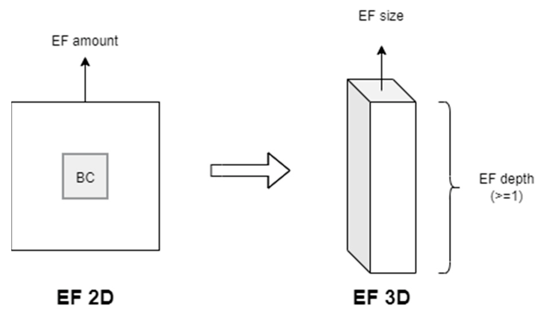
2.2. Three-Dimensional Ecological Footprint Model

EF is an indicator based on the consumption of EF-related products. There are many EF accounting methods, mainly from the perspective of production (EF = EF of local production + EF of import product conversion-EF of export product conversion) and from the perspective of consumption. The former is more suitable for ecological footprint accounting at a national scale and with detailed import and export data, while the latter is more suitable for EF accounting at small scales such as cities and counties. Based on this, the EF accounting in this paper is from the consumption of EF accounting; the EF of arable land, forestland, grassland, and fishing land can be accounted for by the following equation:

$$EF={\displaystyle \sum }_i\frac{C_i}{Y_i}·Y{F}_i·EQ{F}_i$$

(1)

where $Y{F}_i$ is the yield factor for product $i$, used to convert the local area to the global average production area, and $EQ{F}_i$ is the equivalence factor for product $i$, used to convert this land type to the global average land type area (global hectare). The built-up footprint is accounted for by transferring its direct land occupation (arable land) into EF. The carbon footprint is accounted for by transferring the necessary carbon uptake land (forestland) into EF. Different from the calculation of EF, the calculation of BC is based on how much productive land there is in the area, converted into the size of a unified unit. The calculation method is as follows [41]:

$$BC={\displaystyle \sum }_i{A}_i·Y{F}_i·EQ{F}_i$$

(2)

The EF accounting step: firstly,

$A_i$ is the bioproductive area for the production of product $i$. Figure 2 demonstrates the conversion from 2D EF to 3D EF. As designed by Niccolucci et al. [16], the 3D EF model is defined as follows:

$$E{F}_{size}=BC$$

(3)

$$E{F}_{depth}=\left\{\begin{array}{c}\frac{EF}{BC} when EF>BC\\ 1 when EF\le BC\end{array}\right.$$

(4)

2.3. LMDI

The logarithmic mean Divisia index (LMDI) has two forms, i.e., the additive form and the multiple form. The additive form and the multiple form are equivalent, and the former is usually used in physical units while the latter is used in indexes for convenient expression [36]. Since this paper intends to compare the difference in the amount of EFD data decomposition between different years, the decomposition in the additive form is more suitable for the research. According to IPAT and its improvements, this paper selected $P$ to represent the population size, $G$ to represent the total GDP, $G_s$ to represent the total GDP of the tertiary industry, and $T_A$to represent the total number of patents to use in the LMDI decomposition.$A=G/P$ obtains the per capita GDP, indicating the affluence$; S=Gs/G$ obtains the proportion of GDP of the tertiary industry, indicating the industrial structure; $T_s=T_A/G_s$ obtains the regional patent authorization per unit of GDP of the tertiary industry as a whole in that year, representing the technological intensity of the tertiary industry; and $E_t=E{F}_{depth}/T_A$ represents the size of the EF depth per unit of patent authorization, representing the intensity of scientific and technological demand for pollution control. The PyLMDI [42] was used to calculate the results in this study. The equation of the LMDI is as follows:

$$E{F}_{depth}=P\frac{G}{P}\frac{G_s}{G}\frac{T_A}{G_s}\frac{E{F}_{depth}}{T_A}=P·A·S·T_s·E_t$$

(5)

The additive form decomposition for this article is as follows:

$$\Delta EFD=EF{D}^t-EF{D}^0=\Delta EF{D}_P+\Delta EF{D}_A+\Delta EF{D}_S+\Delta EF{D}_{T_s}+\Delta EF{D}_{E_t}$$

(6)

For a general explanation of those sectors, $\Delta EF{D}_X$ is expanded below:

$$\Delta EF{D}_X={\displaystyle \sum }_i\frac{EF{D}_i^t-EF{D}_i^0}{\ln \left(\frac{EF{D}_i^t}{EF{D}_i^0}\right)}·ln\frac{X_i^T}{X_i^0}$$

(7)

X could be $P$, $A$, $S$, $T_s$, or $E_t$in this article, and $i$ is the economic department.

3. Results

3.1. Result of Jiangsu’s Ecological Footprint Depth

The results of the figures below were drawn by ggplot2 [43]. The calculation results showed that the EFD increased from 2.10 in 1995 to 6.28 in 2015 in terms of changes in the entirety of Jiangsu Province. In the research years, in terms of changes per 5 years, EFD increased by 17% (2.10→2.46) in 1995–2000, the lowest growth rate in the 20 years. The growth rate of the EFD reached the largest in 2000–2005, with an increase of 64.4% (2.46→4.05), and the rates in 2005–2010 and 2010–2015 gradually decreased, reaching 31.1% (4.05→5.31) and 18.4% (5.31→6.28), respectively. To better reflect the evolution of the EFD in prefecture-level cities and districts and counties under their jurisdiction, the following analysis was carried out at two regional scales.

From the perspective of the prefecture-level city scale, the evolution of the EFD of 13 prefecture-level cities in Jiangsu Province from 1995 to 2015 is shown in Figure 3 and

Table A1. EFDs of prefecture-level cities of Jiangsu in 1995–2015.

Prefecture-Level Cities	1995	2000	2005	2010	2015
Nanjing	4.22	4.89	7.93	10.57	10.98
Wuxi	4.49	5.53	9.85	12.91	13.42
Xuzhou	2.02	2.34	3.50	4.03	5.69
Changzhou	2.98	3.15	5.84	7.82	9.39
Suzhou	3.23	4.31	10.02	15.69	17.62
Nantong	1.89	2.24	3.73	4.83	6.60
Lianyungang	1.37	1.44	2.01	2.56	4.79
Huaian	1.33	1.59	2.12	2.84	3.45
Yancheng	1.16	1.52	2.20	2.56	3.03
Yangzhou	1.95	2.15	3.43	4.34	4.10
Zhenjiang	2.85	3.16	5.42	6.41	6.86
Taizhou	2.11	2.09	2.98	3.84	4.11
Suqian	1.44	1.61	2.15	2.56	3.75

. The location heights in the figure represent the EFD values of the corresponding city. It can be seen that in the study years, the EFD presents a spatial distribution pattern of high values in the south and low values in the north. In 1995, the regional-level cities showed relatively low differential EFD distributions, among which the EFDs of Nanjing and Wuxi were significantly higher, reaching 4.22 and 4.49, respectively. From 1995 to 2005, the change was small, and the distribution did not change significantly. From 2000–2005, the EFD of the prefecture-level cities underwent relatively significant changes, and Suzhou especially experienced significant growth, increasing 5.71. The main feature of change in 2005–2010 was that the EFD in all cities increased significantly. In 2010–2015, the most obvious change in the EFD was in Lianyungang.

At the county scale, the three-dimensional map of the ecological footprint depth of each county in Jiangsu Province from 1995 to 2015 is shown in Figure 4 and

Table A2. EFDs of counties of Jiangsu in 1995–2015.

Prefecture-Level Cities	County-Level Units	1995	2000	2005	2010	2015
Nanjing	Nanjing Urban	27.89	32.79	46.77	51.88	42.95
	Pukou District	1.13	1.31	3.69	6.25	7.83
	Jiangning District	1.93	2.33	4.45	6.36	9.64
	Liuhe District	1.37	1.41	3.38	6.73	6.19
	Lishui District	1.38	1.50	2.11	3.76	5.05
	Gaochun District	1.63	1.86	3.08	5.40	6.42
Wuxi	Wuxi Urban	7.74	8.80	11.77	12.67	12.51
	Jiangyin City	4.23	6.16	16.70	26.89	29.48
	Yixing City	1.92	2.41	4.13	5.11	5.20
Xuzhou	Xuzhou Urban	14.38	16.41	32.10	31.19	31.15
	Tongshan District	1.21	1.93	2.29	3.18	6.07
	Jiawang District	1.74	1.97	2.80	3.41	5.52
	Fengxian County	1.47	1.52	1.92	2.35	3.82
	Peixian County	2.40	2.32	3.43	3.92	5.95
	Suining County	1.32	1.52	1.99	2.35	3.52
	Xinyi City	1.44	1.59	2.11	2.76	4.30
	Pizhou City	1.39	1.67	2.20	2.98	4.20
Changzhou	Changzhou Urban	7.70	8.27	14.20	18.92	19.78
	Wujin District	3.23	3.47	6.80	10.11	13.56
	Liyang City	1.50	1.48	3.31	4.39	5.21
	Jintan District	1.77	1.90	2.88	3.19	4.03
Suzhou	Suzhou Urban	6.74	8.17	12.93	25.11	26.93
	Wujiang District	2.12	3.15	6.73	10.11	10.63
	Wuzhong District	2.96	4.03	9.13	11.74	12.06
	Changshu City	4.67	4.43	9.43	12.56	17.59
	Zhangjiagang City	2.40	5.14	13.02	24.19	28.81
	Kunshan City	2.22	3.20	10.22	12.58	13.77
	Taicang City	1.73	2.85	10.18	18.82	18.10
Nantong	Nantong Urban	19.43	22.46	38.85	41.45	48.31
	Tongzhou District	1.69	2.07	3.18	3.77	9.04
	Haian County	1.40	1.72	2.79	4.54	5.99
	Rudong County	1.00	1.19	2.17	2.66	3.61
	Qidong City	1.31	1.45	2.11	3.15	4.31
	Rugao City	1.32	1.53	2.53	4.18	4.52
	Haimen City	1.91	2.32	4.14	5.71	6.57
Lianyungang	Lianyungang Urban	4.11	4.33	6.67	7.57	20.50
	Ganyu County	1.27	1.21	1.70	3.27	5.94
	Donghai County	1.00	1.00	1.15	1.30	1.72
	Guanyun County	1.00	1.10	1.36	1.28	1.36
	Guannan County	1.21	1.26	1.69	2.60	3.90
Huaian	Huai’an Urban	5.07	6.13	9.83	15.27	24.44
	Huai’an District	1.73	1.98	2.60	2.98	2.84
	Huaiyin District	1.44	1.74	2.38	3.11	3.71
	Lianshui County	1.00	1.18	1.38	1.91	2.27
	Hongze County	1.15	1.30	1.70	2.41	2.67
	Xuyi County	1.00	1.00	1.11	1.43	1.68
	Jinhu County	1.04	1.27	1.38	1.91	1.93
Yancheng	Yancheng Urban	2.30	3.16	4.46	5.11	5.00
	Xiangshui County	1.00	1.07	1.42	2.13	2.61
	Binhai County	1.00	1.12	1.61	1.91	2.36
	Funing County	1.26	1.67	2.57	2.73	3.38
	Sheyang County	1.00	1.21	1.48	2.27	3.03
	Jianhu County	1.56	2.22	3.18	2.97	2.65
	Dongtai City	1.07	1.32	2.33	2.51	2.72
	Dafeng District	1.00	1.09	1.54	1.63	2.72
Yangzhou	Yangzhou Urban	4.11	4.75	5.44	6.53	6.51
	Jiangdu District	1.95	2.23	5.97	7.99	6.35
	Baoying County	1.27	1.35	1.61	1.75	1.62
	Yizheng City	2.13	2.19	3.57	4.88	4.98
	Gaoyou City	1.16	1.21	1.45	1.68	2.52
Zhenjiang	Zhenjiang Urban	4.75	5.17	13.91	15.28	15.77
	Danyang City	3.06	3.45	3.26	4.71	4.97
	Yangzhong City	2.70	3.09	3.70	5.14	5.20
	Jurong City	1.40	1.57	1.56	1.93	2.10
Taizhou	Taizhou Urban	3.50	5.63	8.92	15.55	17.45
	Jiangyan City	2.46	1.90	2.50	2.74	2.84
	Xinghua City	1.11	1.12	1.58	1.89	2.05
	Jingjiang City	3.17	3.01	4.32	4.58	5.72
	Taixing City	2.66	2.29	3.16	3.74	3.38
Suqian	Suqian Urban	1.90	2.23	3.49	4.54	6.52
	Shuyang County	1.47	1.71	2.16	2.67	4.12
	Siyang County	1.67	1.78	2.09	2.22	2.96
	Sihong County	1.00	1.00	1.25	1.31	2.02

. The overall spatial correlation also gradually increased in the study years. From the perspective of spatial agglomeration, most of the counties are low-EFD agglomeration areas, which are distributed in the northern and central parts of Jiangsu, and high-EFD agglomeration areas are mainly distributed in southern Jiangsu. Due to the process of urbanization, the population is gradually agglomerating in urban areas, and high values are mainly distributed in urban areas of prefecture-level cities, showing a very high EFD that was significantly higher than that of non-urban territorial units.

From 1995 to 2000, the EFDs of a small number of counties decreased, namely, the EFDs of Jiangyan City, Taixing City, Changshu City, Jingjiang City, Peixian County, Ganyu County, and Liyang City. The EFDs of Donghai County, Xuyi County, and Sihong County were unchanged at 1 because their EFs were less than the corresponding BC for each county. During this period, 12 counties increased their EFD by 1, and 7 were prefecture-level urban areas, namely, Nanjing Urban, Nantong Urban, Taizhou Urban, Xuzhou Urban, Suzhou Urban, Wuxi Urban, and Huai’an Urban Areas. Others were economically developed districts and counties in southern Jiangsu: Zhangjiagang City, Jiangyin City, Taicang City, Wuzhong District, and Wujiang District. In addition, counties such as Jianhu County, Kunshan City, and Tongshan District had a faster EFD growth rate.

From 2000 to 2005, there were 34 counties whose EFD growth changed by more than 1, most of which were distributed in urban areas and counties in southern Jiangsu. The higher changes were mainly Zhenjiang urban area (+8.74), Jiangyin City (+10.53), Nanjing Urban Area (+13.97), Xuzhou Urban Area (+15.69), and Nantong Urban Area (+16.39). Some districts and counties experienced little change, such as Danyang City, Jurong City, Jinhu County, Xuyi County, and Donghai County.

From 2005 to 2010, the growth slowed significantly. Some counties that grew rapidly in the first half of the study period hardly changed or even decreased in this range. These include Xuzhou Urban Area and Nantong Urban Area. Most of the districts and counties with large EFD growth are mainly concentrated in the central and southern regions, including Liuhe District, Suzhou Urban Area, Ganyu County, Zhangjiagang City, Taicang City, and Lishui District.

From 2010 to 2015, the overall growth of the EFD in each county further slowed, and 12 counties experienced negative growth, e.g., Jiangdu District, Nanjing Urban Area, Jianhu County, Taixing City, and Liuhe District. Figure 5 shows the distribution of changes in the overall EFDs, and most of them were between 0 and 0.5 for this period. The counties with high values higher than 1 include Lianyungang Urban Area and Tongzhou District. Other high values are obviously smaller than the changes between 2005 and 2010.

3.2. LDMI Results of EF Depth

The following study analyses the influence of the five factors$—A$, $E_t$, $P$, $S$, and $T_s$—on the EFD changes in Jiangsu Province in each time period from the provincial, prefecture-level city, and county levels. We decompose the EFD changes under each influencing factor.

Figure 6 shows the decomposition of the overall EFD change in Jiangsu Province with LMDI. It can be seen from the figure that $E_t$ in each study period had the main negative effect on the change in EFD, and the $A$ and $P$ factors both showed a positive effect on the change in EFD. The $S$ factor showed a weak negative influence (−0.093) in 2000–2005 and a positive influence in the other years. The $T_s$factor showed a positive influence in the first three five-year interval changes; however, in 2010–2015, it had a negative impact, and the EFD decomposition reached −0.721. The $E_t$ factor showed a negative impact in each time period of the study, of which the negative impact was greatest from 2005 to 2010 (−8.689). In 2005–2010, all factors except $S$ showed a stronger influence than in other time periods; however, the EFD changes in this stage were not the highest, indicating that the positive and negative influences of factors such as affluence, population, technology level of the tertiary industry, and the intensity of science and technology demand for pollution control varied relatively greatly at this time, and many of the positive and negative effects offset one another.

The decompositions of EFD changes in 13 prefecture-level cities are shown in Figure 7. And the summary of factors’ decomposition for 13 prefecture-level cities of Jiangsu is shown in

Table A3. Summary of factors’ decomposition for 13 prefecture-level cities of Jiangsu.

	Years Range	Mean	Median	SD	Minimum	Maximum
P	1995–2000	0.15	0.09	0.15	−0.07	0.40
	2000–2005	0.19	−0.01	0.34	−0.09	0.75
	2005–2010	0.56	−0.04	1.20	−0.13	4.08
	2010–2015	0.11	0.06	0.11	−0.01	0.30
A	1995–2000	1.21	1.08	0.56	0.59	2.35
	2000–2005	2.22	1.75	1.30	0.77	4.74
	2005–2010	3.15	2.73	1.44	1.68	6.06
	2010–2015	3.30	2.72	1.78	1.61	7.21
S	1995–2000	0.44	0.46	0.16	0.21	0.77
	2000–2005	−0.08	−0.09	0.44	−1.20	0.63
	2005–2010	0.78	0.45	0.85	0.25	3.36
	2010–2015	1.07	1.01	0.67	0.20	2.69
Ts	1995–2000	1.77	1.80	1.60	−1.72	4.91
	2000–2005	0.20	0.01	0.79	−0.92	2.06
	2005–2010	5.99	3.06	6.39	0.30	21.70
	2010–2015	0.09	0.77	2.82	−4.54	5.42
Et	1995–2000	−3.19	−3.21	1.42	−6.59	−0.85
	2000–2005	−0.58	−0.50	1.02	−2.71	1.64
	2005–2010	−8.96	−5.52	7.94	−27.67	−1.80
	2010–2015	−3.58	−4.52	3.55	−11.78	1.86

. The decompositions of each factor from 1995 to 2000 were relatively balanced among the prefecture-level cities. It is obvious that the main negative influence of EFD at this stage was$E_t$ (mean: −3.186); although $T_s$ had a negative effect in Nanjing (−1.717), its overall positive effect was the largest among these factors, and a positive effect was also found for $P$, $S$, $A$, which had a positive impact on most of these cities. From 2000 to 2005, the situation changed variously compared with that in the previous five years: Factor$A$ became the main positive influencing factor, and $P$, $S$, and $T_s$ showed a relatively uniform positive and negative influence on the number of cities affected; that is, the negative effect became stronger. The $E_t$ factor was still the most negative influencing factor, showing a positive impact in three cities, namely, Changzhou (0.337), Suzhou (1.638), and Nantong (0.03). It can be seen that on the whole, these 13 cities in the time period also had the largest change in EFD compared with other time periods, but the overall variation was small, mainly due to the overall decrease in the absolute value of negative factors. From 2005 to 2010, the absolute value of the influence of various factors increased, especially in Changzhou, Nanjing, Nantong, Suzhou, and Wuxi, cities with relatively developed economies in Jiangsu. The main positive influencing factors were $Ts$, $A$, and $S$, and the influence of EFD was positive in all cities. $T_s$ was the most important positive influencing factor, and P had a positive impact on Suzhou (4.082), Nanjing (1.371), and Wuxi (1.468), which was due to the positive population growth (immigration) of these cities during this period. The largest negative factor in each city was $E_t$. From 2010 to 2015, the absolute value of the overall influencing factors decreased, and the most important positive influencing factor became $A$, followed by $S$. $P$ was positive except in Yancheng (−0.015), but the influence became very small (mean: 0.108); $T_s$ and $E_t$ both showed positive and negative influences in 13 cities; the former mainly had a positive influence, and the largest negative influence factor was still $E_t$.

The results at the county level are shown in Figure 8. And the summary of factors’ decomposition for 73 counties in Jiangsu is shown in

Table A4. Summary of factors’ decomposition for 73 counties in Jiangsu.

	Years Range	Mean	Median	SD	Minimum	Maximum
P	1995–2000	0.23	0.05	0.68	−0.88	4.56
	2000–2005	0.33	−0.03	1.04	−0.49	6.63
	2005–2010	0.66	−0.03	1.86	−2.24	11.40
	2010–2015	0.19	0.02	0.63	−0.98	4.49
A	1995–2000	1.42	0.90	1.99	−0.07	12.90
	2000–2005	2.57	1.49	3.32	0.42	23.37
	2005–2010	3.87	2.22	4.84	0.61	25.08
	2010–2015	3.98	2.40	4.43	0.79	24.99
S	1995–2000	0.44	0.38	0.68	−3.29	3.17
	2000–2005	0.02	0.00	1.18	−3.49	6.30
	2005–2010	0.93	0.34	1.90	−1.31	11.21
	2010–2015	1.41	0.73	1.83	−0.02	10.37
Ts	1995–2000	1.89	1.77	5.21	−31.24	17.26
	2000–2005	0.49	0.04	3.50	−5.38	28.11
	2005–2010	6.36	2.16	16.60	−4.10	132.00
	2010–2015	−0.37	0.44	6.78	−31.36	25.04
Et	1995–2000	−3.49	−2.70	5.39	−25.56	26.73
	2000–2005	−1.05	−0.55	4.57	−36.28	3.72
	2005–2010	−10.06	−3.92	21.68	−165.88	0.08
	2010–2015	−4.01	−2.61	9.50	−61.99	21.52

. The results show that the decompositions of EFDs in Jiangsu’s counties showed great changes in time and space with the five factors.

From 1995–2000, there were three counties with EFDs equal to 1 because each EF was smaller than the corresponding BC, i.e., Donghai County, Xuyi County, and Sihong County. There was no change during this period for the three counties, and the figure shows that the factor change was 0. There were three change factors with a more obvious decomposition effect, i.e., $A$, $S$, and $P$. $A$showed a stronger positive effect, and the decomposition values were all positive. $A$ had the largest average value of the decomposition amount of the EFD change at this stage, which is 1.422. $S$ mainly showed a positive decomposition effect, with an average decomposition of EFD changes of 0.439. $P$ generally had positive effects, with an average decomposition value of 0.225. At this stage, there were only 16 counties for $P$ with a negative effect, and the absolute value of the number was small. In addition, $T_s$ showed more negative effects, and $E_t$ showed both positive and negative effects.

From 2000 to 2005, the absolute and relatively significant values of the influencing factors in the 73 counties were mainly in Nanjing Urban Area and Nantong Urban Area. Similar to the order of the main influencing factors of prefecture-level cities, the most important positive influencing factor in this period was also $A$. The positive and negative effects of the four factors varied in different counties. On the whole, there were more counties with $T_s$, $P$, and $S$ showing a positive effect and more counties with a negative effect from $E_t$.

From 2005 to 2010, except for $A$, which only showed a positive influence factor, all other factors showed both positive and negative influence factors. $T_s$ was the main positive influence factor, $E_t$ showed a relatively strong negative influence, and there was only one unit, Wujiang District (0.077), that showed a positive effect. The number of counties negatively affected by the population factor reached 42, mainly due to the decrease in population in these areas during this period, mainly in central and northern Jiangsu, such as Jiangyan City, Taixing City, Suining County, Sheyang County, and Guanyun County. In addition, the $S$ factor mainly had a positive effect, reaching 63 counties.

From 2010 to 2015, $A$ again became the main positive influencing factor. Among the 73 geographic units, Nantong (24.989) and Nanjing (22.786) showed a larger decomposition value performance. Due to the change in population distribution, $P$ also showed a phenomenon with both positive and negative impacts; however, the absolute value of the impact was relatively low except for a few counties, among which counties with the highest positive impact were Xuzhou Urban Area (4.494), Huai’an Urban Area (1.716), Nanjing Urban Area (1.574), and Lianyungang Urban Area (1.113). Compared with the previous stage, the positive effect of the $S$ factor increased, the negative effect of $T_s$ increased (34 negatively affected counties), and the positive effect of$E_t$ increased (17 positively affected counties).

4. Discussion

A discussion of EFD differences and the factor decomposition effects at different scales is necessary. From the research results at the provincial, prefecture-city level, and district and county levels, it can be seen that when different scales are unfolded layer by layer, the finer the geographical units are, the greater the difference in EFD changes and factor decomposition. The finer the regional scale is, the greater the heterogeneity. The data at the provincial level and the prefecture-level city scale show little change, which is mainly reflected in the different distributions between the north and south of the prefecture-level cities. The county-level data not only showed the difference between the north and the south but also highlighted the significant differences between the urban areas and non-urban areas. In terms of the absolute value of the factor decomposition of each county, the urban areas are also significantly higher than the value of the non-urban areas. Due to the agglomeration effect of urbanization population, economy, and other factors in large cities, the population density of prefecture-level urban areas was significantly higher than that of surrounding districts and counties, and the population size gap between regions was large. There were some differences in the impact of population factors at different scales: from the perspective of 20-year temporal and spatial changes, the overall impact of population factors on EFD in Jiangsu Province decreased, while from the perspective of prefecture-level cities and counties, especially from 2005 to 2010, the factors affecting the population increased in some regions. This was due to the migration of the population between regions brought about by urbanization, especially the migration of the population from districts and counties to prefecture-level cities at the same level. This finding shows that urbanization will affect the ecological pressure of developed regions to a certain extent.

From the perspective of counties, the results of the regression analysis to study the relationship between EFD and explanatory variables can be explained from the regression coefficient, and the decomposition method mainly gives the decomposition value of the change in EFD caused by the change in decomposing factors. The correlation analysis of each decomposition factor and EFD is shown in Figure 9. It can be seen that in the research years, population size, affluence, industrial structure, and depth of ecological footprint mainly showed a significant positive correlation, while the relationships between the level of science and technology in the tertiary industry, the intensity of scientific and technological demand for pollution control, and EFD were diverse. As defined in Equation (7), for EF as a whole to input into the equation, the direction of change of positive and negative change in the same direction is shown in Figure 10, and the points are all located in the first and third quadrants. The relationship of the change in each factor and the change in EFD and the relationship between each factor and EFD show similar characteristics: the respective differences in population size, affluence, and industrial structure have a strong correlation with the corresponding decomposition of EFD in each time stage, while $\Delta T_s$ and $\Delta E_t$ have a weak relationship with the corresponding decomposition amount of EFD. This weak relationship presents a variety of relationships at the county scale. It plays a relatively important decomposition role in some counties, and the influence of the EFD was less stable. In some cases, EFD has a positive impact, and in some cases a negative impact. $E_t$, such as in the Nantong Urban Area, had a strong negative impact on the EFD from 2005 to 2010, and from 2010 to 2015 the influence became positive. At the same time, it can be seen that the scale of EFD change and the scale of factor decomposition do not necessarily have a corresponding relationship. For example, the largest change in EFD at the county level was from 2000–2005 (average change 2.36), and the largest change in factor differences was between 2005 and 2010, e.g., the positive effect of $S$ showed a wave-time development, decreasing from 1995 to 2005, and the positive effect of $S$ gradually increased from 2005 to 2015, while its negative effect gradually decreased.

From the comparative discussion of the literature findings, there is no EF literature from the perspective of EFD in Jiangsu Province, and there are findings in Jiangsu Province mainly from the provincial scale EF [44,45]. The results of the previous studies indicate the overall trend of increasing ecological pressure in Jiangsu province, and the results of this study are clearer about the ecological pressure distribution and driving factors. In analysis of the results of other related 3D EF studies [22,25], most of the EFD results have a larger scale of geographic units. Comparative analysis shows that this study is better able to show the 3D EF of each regional unit and to respond to spatial information, and it is easy to carry out the evaluation of ecological pressure and ecological balance within the city. The results of this study differ significantly from other studies in terms of the effects of demographic factors on EFD [25], partly due to model variability and partly due to variability between regions. The analysis of GDP (GDP per capita) results [20,21] has similar conclusions to most studies and serves as a major positive driver, showing more clearly the difference in the impact of GDP on EFD over the study year range than most studies. In conclusion, there are differences in other factors, and the overall difference in the study in terms of influence factors and interactions is obvious in time and space between regions, highlighting the degree of subdivision of the influencing factors in different regions and different periods.

5. Conclusions and Policy Implications

5.1. Conclusions

In this article, the focus points are the distribution and changes in Jiangsu’s EFDs and the decomposition of the EFD changes with influencing factors. The following conclusions are drawn:

(1)

Multi-scale EFD research in Jiangsu Province can mine ecological information at different geographic scales and compare differences and scales, which can provide support for the study of ecological balance between and within regions. At the county scale, the unbalanced north–south difference in the EFD distribution increases year by year, and the difference between the urban areas and the counties is obvious.

(2)

The factor decomposition method divides the factors of each time interval of EFD in Jiangsu Province. Affluence was the most important decomposing factor, which has always been shown to affect the change in EFDs at different scales, different regions, and different time periods. Other factors all showed the effect of diversity and quality in the above three conditions, among which the factor of the ratio of EFD to technological level was the main inhibitory factor. The annual factor changes have certain differences in geographical units at different scales. Industrial structure and population factors mainly showed the promoting effect of EFD, while the technological intensity of the tertiary industry has a relatively large heterogeneous effect on EFD.

(3)

Finally, this paper discusses the relationship between factors in a targeted manner and proposes countermeasures and suggestions to reduce EFD and balance the ecological pressure among regions from multiple perspectives.

5.2. Policy Implications

In view of the results of EFD and factor zoning in Jiangsu Province, to reduce EFD and balance the ecological pressure among regions, the following countermeasures are suggested:

(1)

The ecological pressure analysis in Jiangsu Province should be conducted at multiple scales, focusing on the balanced distribution of the population and the balance of ecological pressure. To this end, it is necessary to pay attention to the balanced development among regions. The transfer and layout of industries from developed counties with high ecological pressure to economically underdeveloped districts and counties with low ecological pressure would help transfer the impact of population factors on EFD and reduce the original high EFD value. The specific implementation can be combined with the research results (Table A1 and Table A2) in this paper for the reference of policymakers, e.g., in 2015, the ecological pressures of Suzhou, Nanjing, Wuxi, Changzhou, Nantong, and Zhenjiang, most of which were in the south of Jiangsu, were significantly higher than those of other prefecture-level cities. Therefore, the industries and population of those cities could be transferred to other cities with small EFDs. At the same time, attention should be given to the integrated urbanization development of prefecture-level cities and districts and counties to increase the city’s overall ecological pressure resistance capability and avoid extreme increases in local ecological pressure caused by agglomeration. Therefore, it is necessary to reasonably optimize their urbanization rates, and to strengthen the construction of rural basic livelihoods, so as to alleviate urban ecological pressures. Within a prefecture-level city, taking Huai’an City for example in 2015, the EFD of the Huai’an Urban reached 24.44, while in the same period, the EFD of non-urban areas under the prefecture-level city was only in the range of 1.68–3.71. Therefore, the high EFD industries in Huai’an Urban Area need to be balanced with other regions, while expanding the attractiveness of non-urban areas within the prefecture-level city and reducing the pressure on the urban area.

(2)

It is recommended to focus on different growth-influencing factors at different stages, because the influencing factors have a certain change pattern at different stages. For example, the population factor has a greater impact in the early stage but has less influence in the later stage. In addition, the heterogeneity of critical influencing factors of EFD among districts and counties should be highlighted to develop differentiated countermeasures to reduce EFD. From the results of the analysis, for example, in 2015, to effectively refrain the growth of EFD, Huai’an Urban should focus on the increase in $T_s$, while Nanjing Urban should focus on the increase in $E_t$.

(3)

The results show that, for most of the regions in Jiangsu, attention should be given to the development mode of the green economy and to optimizing the industrial structure to reduce the impact of economic growth and the economic structure on EFD. In addition, a focus should be on improving the GDP output of the tertiary industry per unit of science and technology and promoting the speed of science and technology development to exceed the growth rate of EFD, which will help reduce EFD at the scales of provinces, cities, districts, and counties.

5.3. Limitations of this Study and Future Study Recommendations

Limitations of this study are the following: (1) Since there is no district/county level input–output table, this paper does not use LMDI to decompose EFD influencing factors based on industry sectors. (2) Due to the fact that this study focuses on the decomposition of EFDs with LMDI, this paper did not conduct a comparative study among multiple decompositions or regression models. (3) There was no analysis on EFDs by land type.

Future study recommendations are the following: (1) It can be suggested that the factor research of EFD can be compared based on LMDI, regression, and other models. (2) The spatial agglomeration effect and heterogeneity of these influencing factors of LMDI can be further studied. (3) The EFDs of different land type could be analyzed further.

References

1. Ahmed, Z.; Asghar, M.M.; Malik, M.N.; Nawaz, K. Moving towards a Sustainable Environment: The Dynamic Linkage between Natural Resources, Human Capital, Urbanization, Economic Growth, and Ecological Footprint in China. Resour. Policy 2020, 67, 101677. [Google Scholar] [CrossRef]
2. Folke, C.; Biggs, R.; Norström, A.V.; Reyers, B.; Rockström, J. Social-Ecological Resilience and Biosphere-Based Sustainability Science. E&S 2016, 21, art41. [Google Scholar] [CrossRef]
3. Steffen, W.; Richardson, K.; Rockström, J.; Cornell, S.E.; Fetzer, I.; Bennett, E.M.; Biggs, R.; Carpenter, S.R.; de Vries, W.; de Wit, C.A.; et al. Planetary Boundaries: Guiding Human Development on a Changing Planet. Science 2015, 347, 1259855. [Google Scholar] [CrossRef] [PubMed] [Green Version]
4. Cheng, H.; Zhu, L.; Meng, J. Fuzzy Evaluation of the Ecological Security of Land Resources in Mainland China Based on the Pressure-State-Response Framework. Sci. Total Environ. 2022, 804, 150053. [Google Scholar] [CrossRef] [PubMed]
5. Wang, Y.; He, X. Spatial Economic Dependency in the Environmental Kuznets Curve of Carbon Dioxide: The Case of China. J. Clean. Prod. 2019, 218, 498–510. [Google Scholar] [CrossRef]
6. Xun, F.; Hu, Y. Evaluation of Ecological Sustainability Based on a Revised Three-Dimensional Ecological Footprint Model in Shandong Province, China. Sci. Total Environ. 2019, 649, 582–591. [Google Scholar] [CrossRef]
7. Kassouri, Y.; Alola, A.A. Towards Unlocking Sustainable Land Consumption in Sub-Saharan Africa: Analysing Spatio-Temporal Variation of Built-up Land Footprint and Its Determinants. Land Use Policy 2022, 120, 106291. [Google Scholar] [CrossRef]
8. Penz, E.; Polsa, P. How Do Companies Reduce Their Carbon Footprint and How Do They Communicate These Measures to Stakeholders? J. Clean. Prod. 2018, 195, 1125–1138. [Google Scholar] [CrossRef]
9. Laroche, P.C.S.J.; Schulp, C.J.E.; Kastner, T.; Verburg, P.H. The Role of Holiday Styles in Shaping the Carbon Footprint of Leisure Travel within the European Union. Tour. Manag. 2023, 94, 104630. [Google Scholar] [CrossRef]
10. Rees, W.E. Ecological Footprints and Appropriated Carrying Capacity: What Urban Economics Leaves Out. Environ. Urban. 1992, 4, 121–130. [Google Scholar] [CrossRef]
11. Wackernagel, M.; Rees, W.E. Our Ecological Footprint: Reducing Human Impact on the Earth; New Society Publishers: Philadelphia, PA, USA, 1996. [Google Scholar]
12. Ruiz-Pérez, M.R.; Alba-Rodríguez, M.D.; Marrero, M. Evaluation of Water Footprint of Urban Renewal Projects. Case Study in Seville, Andalusia. Water Res. 2022, 221, 118715. [Google Scholar] [CrossRef]
13. Razzaq, A.; Ajaz, T.; Li, J.C.; Irfan, M.; Suksatan, W. Investigating the Asymmetric Linkages between Infrastructure Development, Green Innovation, and Consumption-Based Material Footprint: Novel Empirical Estimations from Highly Resource-Consuming Economies. Resour. Policy 2021, 74, 102302. [Google Scholar] [CrossRef]
14. Jia, Z.; Wen, S.; Liu, Y. China’s Urban-Rural Inequality Caused by Carbon Neutrality: A Perspective from Carbon Footprint and Decomposed Social Welfare. Energy Econ. 2022, 113, 106193. [Google Scholar] [CrossRef]
15. Niccolucci, V.; Galli, A.; Reed, A.; Neri, E.; Wackernagel, M.; Bastianoni, S. Towards a 3D National Ecological Footprint Geography. Ecol. Model. 2011, 222, 2939–2944. [Google Scholar] [CrossRef]
16. Niccolucci, V.; Bastianoni, S.; Tiezzi, E.B.P.; Wackernagel, M.; Marchettini, N. How Deep Is the Footprint? A 3D Representation. Ecol. Model. 2009, 220, 2819–2823. [Google Scholar] [CrossRef]
17. Mancini, M.S.; Galli, A.; Niccolucci, V.; Lin, D.; Hanscom, L.; Wackernagel, M.; Bastianoni, S.; Marchettini, N. Stocks and Flows of Natural Capital: Implications for Ecological Footprint. Ecol. Indic. 2017, 77, 123–128. [Google Scholar] [CrossRef]
18. Bi, M.; Yao, C.; Xie, G.; Liu, J.; Qin, K. Improvement and Application of the Three-Dimensional Ecological Footprint Model. Ecol. Indic. 2021, 125, 107480. [Google Scholar] [CrossRef]
19. Yang, Y.; Cai, Z. Ecological Security Assessment of the Guanzhong Plain Urban Agglomeration Based on an Adapted Ecological Footprint Model. J. Clean. Prod. 2020, 260, 120973. [Google Scholar] [CrossRef]
20. Tang, Y.; Wang, M.; Liu, Q.; Hu, Z.; Zhang, J.; Shi, T.; Wu, G.; Su, F. Ecological Carrying Capacity and Sustainability Assessment for Coastal Zones: A Novel Framework Based on Spatial Scene and Three-Dimensional Ecological Footprint Model. Ecol. Model. 2022, 466, 109881. [Google Scholar] [CrossRef]
21. Yang, Y.; Lu, H.; Liang, D.; Chen, Y.; Tian, P.; Xia, J.; Wang, H.; Lei, X. Ecological Sustainability and Its Driving Factor of Urban Agglomerations in the Yangtze River Economic Belt Based on Three-Dimensional Ecological Footprint Analysis. J. Clean. Prod. 2022, 330, 129802. [Google Scholar] [CrossRef]
22. Li, X.; Xiao, L.; Tian, C.; Zhu, B.; Chevallier, J. Impacts of the Ecological Footprint on Sustainable Development: Evidence from China. J. Clean. Prod. 2022, 352, 131472. [Google Scholar] [CrossRef]
23. Chen, Y.; Lu, H.; Yan, P.; Qiao, Y.; Xia, J. Spatial-Temporal Collaborative Relation among Ecological Footprint Depth/Size and Economic Development in Chengyu Urban Agglomeration. Sci. Total Environ. 2022, 812, 151510. [Google Scholar] [CrossRef] [PubMed]
24. Li, P.; Zhang, R.; Xu, L. Three-Dimensional Ecological Footprint Based on Ecosystem Service Value and Their Drivers: A Case Study of Urumqi. Ecol. Indic. 2021, 131, 108117. [Google Scholar] [CrossRef]
25. Dong, H.; Li, P.; Feng, Z.; Yang, Y.; You, Z.; Li, Q. Natural Capital Utilization on an International Tourism Island Based on a Three-Dimensional Ecological Footprint Model: A Case Study of Hainan Province, China. Ecol. Indic. 2019, 104, 479–488. [Google Scholar] [CrossRef]
26. Marrero, M.; Puerto, M.; Rivero-Camacho, C.; Freire-Guerrero, A.; Solís-Guzmán, J. Assessing the Economic Impact and Ecological Footprint of Construction and Demolition Waste during the Urbanization of Rural Land. Resour. Conserv. Recycl. 2017, 117, 160–174. [Google Scholar] [CrossRef]
27. Wu, Y.; Zhang, T.; Zhang, H.; Pan, T.; Ni, X.; Grydehøj, A.; Zhang, J. Factors Influencing the Ecological Security of Island Cities: A Neighborhood-Scale Study of Zhoushan Island, China. Sustain. Cities Soc. 2020, 55, 102029. [Google Scholar] [CrossRef]
28. Kovács, Z.; Harangozó, G.; Szigeti, C.; Koppány, K.; Kondor, A.C.; Szabó, B. Measuring the Impacts of Suburbanization with Ecological Footprint Calculations. Cities 2020, 101, 102715. [Google Scholar] [CrossRef]
29. Nathaniel, S.; Khan, S.A.R. The Nexus between Urbanization, Renewable Energy, Trade, and Ecological Footprint in ASEAN Countries. J. Clean. Prod. 2020, 272, 122709. [Google Scholar] [CrossRef]
30. Wu, X.; Zhang, J.; Zhang, D. Explore Associations between Subjective Well-Being and Eco-Logical Footprints with Fixed Effects Panel Regressions. Land 2021, 10, 931. [Google Scholar] [CrossRef]
31. York, R.; Rosa, E.A.; Dietz, T. STIRPAT, IPAT and ImPACT: Analytic Tools for Unpacking the Driving Forces of Environmental Impacts. Ecol. Econ. 2003, 46, 351–365. [Google Scholar] [CrossRef]
32. Aydin, C.; Esen, Ö.; Aydin, R. Is the Ecological Footprint Related to the Kuznets Curve a Real Process or Rationalizing the Ecological Consequences of the Affluence? Evidence from PSTR Approach. Ecol. Indic. 2019, 98, 543–555. [Google Scholar] [CrossRef]
33. Ke, H.; Dai, S.; Yu, H. Spatial Effect of Innovation Efficiency on Ecological Footprint: City-Level Empirical Evidence from China. Environ. Technol. Innov. 2021, 22, 101536. [Google Scholar] [CrossRef]
34. Lv, T.; Zeng, C.; Stringer, L.C.; Yang, J.; Wang, P. The Spatial Spillover Effect of Transportation Networks on Ecological Footprint. Ecol. Indic. 2021, 132, 108309. [Google Scholar] [CrossRef]
35. Ang, B.W. The LMDI Approach to Decomposition Analysis: A Practical Guide. Energy Policy 2005, 33, 867–871. [Google Scholar] [CrossRef]
36. Ang, B.W. LMDI Decomposition Approach: A Guide for Implementation. Energy Policy 2015, 86, 233–238. [Google Scholar] [CrossRef]
37. Pu, Z.; Fu, J.; Zhang, C.; Shao, J. Structure Decomposition Analysis of Embodied Carbon from Transition Economies. Technol. Forecast. Soc. Chang. 2018, 135, 1–12. [Google Scholar] [CrossRef]
38. Li, W.; Xu, D.; Li, G.; Su, B. Structural Path and Decomposition Analysis of Aggregate Embodied Energy Intensities in China, 2012-2017. J. Clean. Prod. 2020, 276, 124185. [Google Scholar] [CrossRef]
39. Zhang, Y.; Shuai, C.; Bian, J.; Chen, X.; Wu, Y.; Shen, L. Socioeconomic Factors of PM2.5 Concentrations in 152 Chinese Cities: Decomposition Analysis Using LMDI. J. Clean. Prod. 2019, 218, 96–107. [Google Scholar] [CrossRef]
40. Burkhard, B.; Kroll, F.; Nedkov, S.; Müller, F. Mapping Ecosystem Service Supply, Demand and Budgets. Ecol. Indic. 2012, 21, 17–29. [Google Scholar] [CrossRef]
41. Borucke, M.; Moore, D.; Cranston, G.; Gracey, K.; Iha, K.; Larson, J.; Lazarus, E.; Morales, J.C.; Wackernagel, M.; Galli, A. Accounting for Demand and Supply of the Biosphere’s Regenerative Capacity: The National Footprint Accounts’ Underlying Methodology and Framework. Ecol. Indic. 2013, 24, 518–533. [Google Scholar] [CrossRef]
42. Xiang, X.; Ma, X.; Ma, Z.; Ma, M.; Cai, W. Python-LMDI: A Tool for Index Decomposition Analysis of Building Carbon Emissions. Buildings 2022, 12, 83. [Google Scholar] [CrossRef]
43. Wickham, H. Ggplot2: Elegant Graphics for Data Analysis; Springer: New York, NY, USA, 2016; ISBN 978-3-319-24277-4. [Google Scholar]
44. Peng, B.; Li, Y.; Elahi, E.; Wei, G. Dynamic Evolution of Ecological Carrying Capacity Based on the Ecological Footprint Theory: A Case Study of Jiangsu Province. Ecol. Indic. 2019, 99, 19–26. [Google Scholar] [CrossRef]
45. He, J.; Wan, Y.; Feng, L.; Ai, J.; Wang, Y. An Integrated Data Envelopment Analysis and Emergy-Based Ecological Footprint Methodology in Evaluating Sustainable Development, a Case Study of Jiangsu Province, China. Ecol. Indic. 2016, 70, 23–34. [Google Scholar] [CrossRef]
Figure 1. The administrative divisions of cities and counties in Jiangsu.
Land 11 01997 g001
Figure 2. From 2D EF to 3D EF.
Land 11 01997 g002
Figure 3. Jiangsu’s city-level ecological footprint depth from 1995–2015.
Land 11 01997 g003
Figure 4. Jiangsu’s county-level ecological footprint depth from 1995–2015.
Land 11 01997 g004
Figure 5. Change values of EFD of counties in Jiangsu Province in 1995–2015.
Land 11 01997 g005
Figure 6. LMDI decomposition of Jiangsu’s overall EFD changes from 1995-2015.
Land 11 01997 g006
Figure 7. LMDI decomposition of Jiangsu’s prefecture-level cities of EFD changes in 1995–2015.
Land 11 01997 g007
Figure 8. LMDI decomposition of the EFD changes in Jiangsu’s counties from 1995–2015.
Land 11 01997 g008
Figure 9. Scatter plots of EFD and factors for 73 counties of Jiangsu in 1995–2015.
Land 11 01997 g009
Figure 10. Relationship between the changes in factors and decomposition of EFD changes in Jiangsu in 1995–2015.
Land 11 01997 g010