


Influence of Different Methods to Estimate the Soil Thermal Properties from Experimental Dataset
 ,
,  and
and
Abstract
1. Introduction
2. Material and Methods
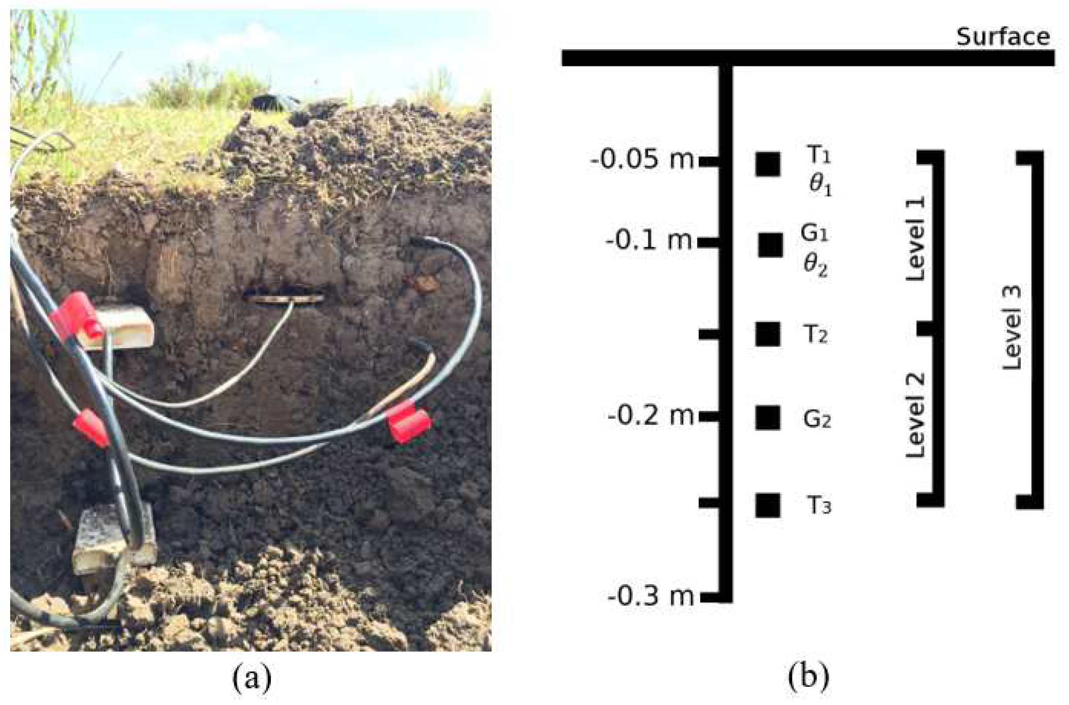
2.1. Site Description and Measurements
2.2. Theoretical Structure
2.2.1. Heat Conduction Equation
- (i)
- Assuming that the soil water content is constant with respect to time and depth, then the thermal conductivity will be independent of the position; consequently, the thermal diffusivity will also be constant and, assuming these conditions, Equation (3) reduces to the particular casewhere the soil thermal diffusivity, (), is independent of depth.
- (ii)
- Assuming that the soil water content varies depending on depth, a term including the influence of soil water content is added in Equation (2); in this case, Equation (3) can be written as follows
2.2.2. Heat Conduction Equation Solutions
Analytical Solution: Amplitude and Phase Shift Methods
Numerical Solution
2.2.3. Empirical Modeling of Thermal Properties as a Function of Soil Water Content
Soil Thermal Conductivity as a Function of Soil Water Content
Soil Thermal Diffusivity as a Function of Soil Water Content
2.3. Evaluated Models/Methods
- -
- : soil thermal conductivity (λ) estimation by the least squares method applied to the numerical solution (Equation (12)), from the daily average of the experimental data of the soil temperature.
- -
- : soil thermal conductivity (λ) estimation by the least squares method applied to the numerical solution (Equation (13)), from the daily average of the experimental data of the soil temperature.
- -
- : soil thermal diffusivity (k) estimation by the Amplitude (Equation (9)) analytical method. The A1 and A2 parameters were fitted to Equation (8) from the daily average soil temperature experimental data, using the least squares method.
- -
- : soil thermal diffusivity (k) estimation by the Phase Shift (Equation 10) analytical method. The and parameters were fitted to Equation (8) from the daily average soil temperature experimental data, using the least squares method.
- -
- : soil thermal diffusivity (k) estimation by the least squares method applied to the numerical solution (Equation (14)), considering the parameter as null ().
- -
- : soil thermal diffusivity (k) and vertical gradient of soil thermal diffusivity () estimation by the least squares method applied to the numerical solution (Equation (14)).
- -
- MTong: soil thermal conductivity estimation as a function of soil water content (Equation (15)). The empirical model proposed by Tong et al. [22].
- -
- MZimmer: soil thermal conductivity estimation as a function of soil water content (Equation (16)). The empirical model proposed by Zimmer et al. [25].
- -
- MAk: soil thermal diffusivity estimation as a function of soil water content (Equation (17)). The empirical–analytical model proposed by Arkhangel’skaya [20].
- -
- MTk: soil thermal diffusivity estimation as a function of soil water content (Equation (18)). The empirical model proposed by Tikhonravova and Khitrov [20].
- -
- MC: soil thermal diffusivity estimation as a function of soil water content, based on a Cubic Polynomial function (Equation (19)). The empirical model suggested in this research.
3. Results
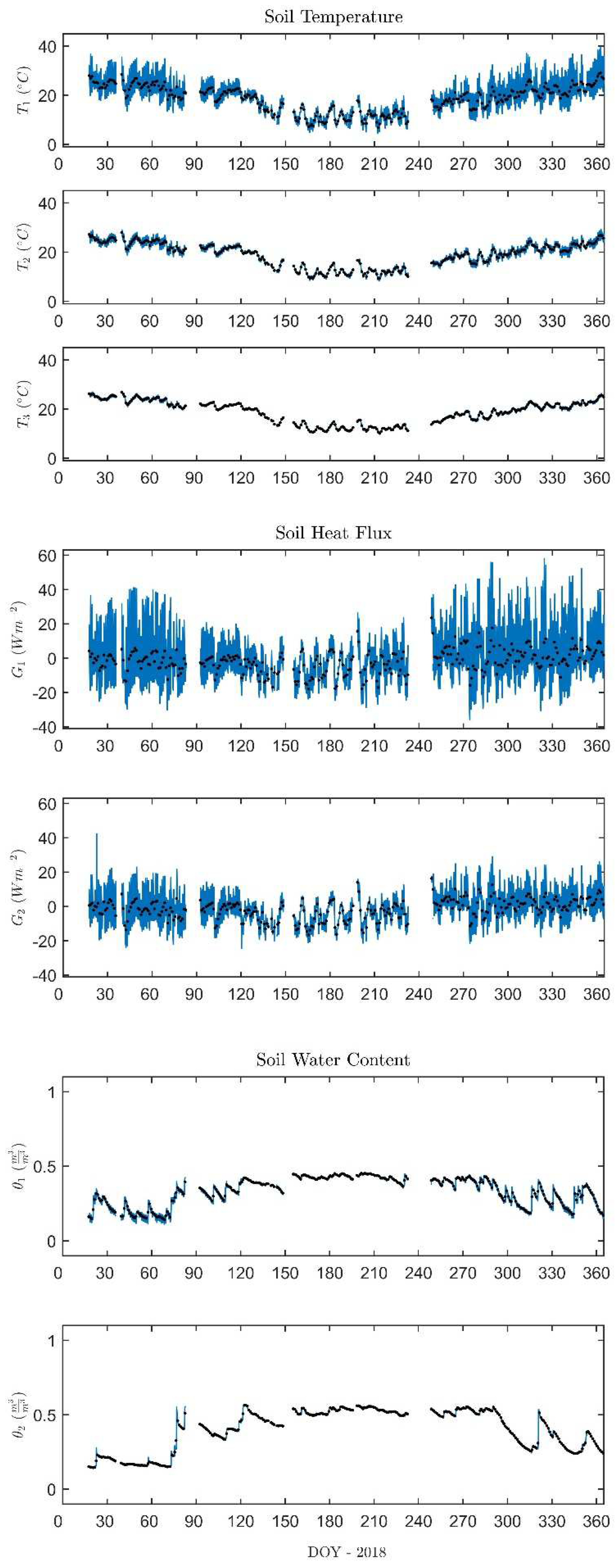
3.1. Soil Variables
3.2. Soil Thermal Properties
3.2.1. Soil Thermal Conductivity
3.2.2. Soil Thermal Diffusivity
3.3. Soil Thermal Properties as a Function of Soil Water Content
3.3.1. Soil Thermal Conductivity
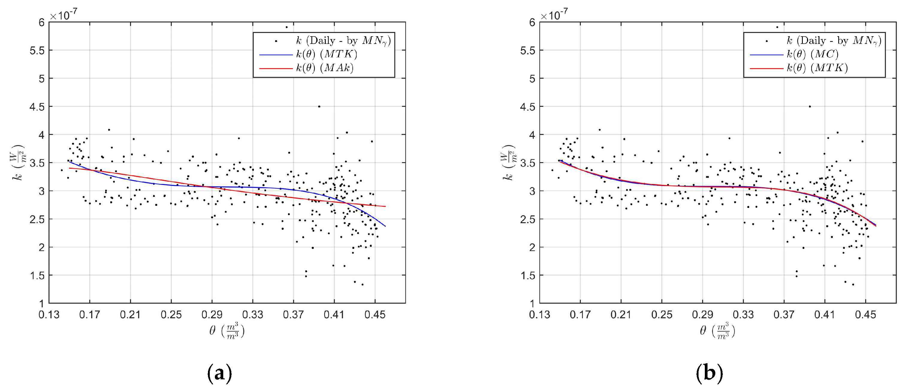
3.3.2. Soil Thermal Diffusivity
4. Discussion
4.1. Soil Thermal Conductivity
4.2. Soil Thermal Diffusivity
4.3. Relationships with Soil Water Content
5. Conclusions
Author Contributions
Funding
Data Availability Statement
Acknowledgments
Conflicts of Interest
References
- Lupatini, M.; Suleiman, A.K.A.; Jacques, R.J.S.; Lemos, L.N.; Pylro, V.S.; Veen, J.A.V.; Kuramae, E.E.; Roesch, L.F.W. Moisture Is More Important than Temperature for Assembly of Both Potentially Active and Whole Prokaryotic Communities in Subtropical Grassland. Microb. Ecol. 2019, 77, 460–470. [Google Scholar] [CrossRef] [PubMed]
- Shukla, M.K. Soil Physics: An Introduction, 1st ed.; CRC Press: Boca Raton, FL, USA, 2014. [Google Scholar]
- Mikhailov, M.D.; Ozisik, M.N. Unified Analysis and Solutions of Heat and Mass Diffusion; Dover Publications: Mineola, NY, SA, 1983. [Google Scholar]
- Gao, Z.; Fan, X.; Bian, L. An Analytical Solution to One-Dimensional Thermal Conduction-Convection in Soil. Soil Sci. 2003, 168, 99–107. [Google Scholar] [CrossRef]
- Gao, Z. Determination of Soil Heat Flux in a Tibetan Short-Grass Prairie. Bound. Layer Meteorol. 2005, 114, 165–178. [Google Scholar] [CrossRef]
- Gao, Z.; Lenschow, D.H.; Horton, R.; Zhou, M.; Wang, L.; Wen, J. Comparison of Two Soil Temperature Algorithms for a Bare Ground Site on the Loess Plateau in China. J. Geophys. Res. 2008, 113, D18105. [Google Scholar] [CrossRef]
- Chen, D.; Kling, J. Apparent Thermal Diffusivity in Soil: Estimation from Thermal Records and Suggestions for Numerical Modeling. Phys. Geogr. 1996, 5, 419–430. [Google Scholar] [CrossRef]
- An, K.; Wang, W.; Wang, Z.; Zhao, Y.; Yang, Z.; Chen, L.; Zhang, Z.; Duan, L. Estimation of Ground Heat Flux from Soil Temperature over a Bare Soil. Theor. Appl. Climatol. 2016, 129, 913–922. [Google Scholar] [CrossRef]
- Carslaw, H.S.; Jaeger, J.C. Conduction of Heat in Solids, 4th ed.; Oxford University Press: London, UK, 1959. [Google Scholar]
- de Vries, D.A. Thermal Properties of Soils. In Physics of Plant Environment; van Wijk, W.R., Ed.; North-Holland Publishing Company: Amsterdam, The Netherlands, 1963. [Google Scholar]
- Wierenga, P.J.; Nielsen, D.R.; Hagan, R.M. Thermal Properties of Soil Based upon Field and Laboratory Measurements. Soil Sci. Soc. Am. Proc. 1969, 33, 354–360. [Google Scholar] [CrossRef]
- Horton, R.; Wierenga, P.J.; Nielsen, D.R. Evaluation of Methods for Determining the Apparent Thermal Diffusivity of Soil Near the Surface. Soil Sci. Soc. Am. J. 1983, 47, 25–32. [Google Scholar] [CrossRef]
- Evett, S.R.; Agam, N.; Kustas, W.P.; Colaizzi, P.D.; Schwartz, R.C. Soil Profile Method for Soil Thermal Diffusivity, Conductivity and Heat Flux: Comparison to Soil Heat Flux Plates. Adv. Water Resour. 2012, 50, 41–54. [Google Scholar] [CrossRef]
- Gao, Z.; Russel, E.S.; Missik, J.E.C.; Huang, M.; Chen, X.; Strickland, C.E.; Clayton, R.; Arntzen, E.; Ma, Y.; Liu, H. A Novel Approach to Evaluate Soil Heat Flux Calculation: An Analytical Review of Nine Methods. J. Geophys. Res. Atmos. 2017, 122, 6934–6949. [Google Scholar] [CrossRef]
- Romio, L.C.; Roberti, D.R.; Buligon, L.; Zimmer, T.; Degrazia, G.A. A Numerical Model to Estimate the Soil Thermal Conductivity Using Field Experimental Data. Appl. Sci. 2019, 9, 4799. [Google Scholar] [CrossRef]
- Stepanenko, V.; Repina, I.; Artamonov, A. Derivation of Heat Conductivity from Temperature and Heat Flux Measurements in Soil. Land 2021, 10, 552. [Google Scholar] [CrossRef]
- Campbell, G.S. Soil Physics with Basic: Transport Models for Soil-Plant Systems. In Developments in Soil Science 14, 1st ed.; Elsevier Science B.V.: Amsterdam, The Netherlands, 1985. [Google Scholar]
- de Vries, D.A. Thermal Conductivity of Soil. Nature 1956, 178, 1074. [Google Scholar] [CrossRef]
- Wang, K.; Wang, P.; Liu, J.; Sparrow, M.; Haginoya, S.; Zhou, X. Variation of Surface Albedo and Soil Thermal Parameters with Soil Moisture Content at a Semi-Desert Site on the Western Tibetan Plateau. Bound. Layer Meteorol. 2005, 116, 117–129. [Google Scholar] [CrossRef]
- Arkhangel’skaya, T.A. Parameterization and Mathematical Modeling of the Dependence of Soil Thermal Diffusivity on the Water. Content Eurasian Soil Sci. 2009, 42, 162–172. [Google Scholar] [CrossRef]
- Lu, Y.; Lu, S.; Horton, R.; Ren, T. An Empirical Model for Estimating Soil Thermal Conductivity from Texture, Water Content, and Bulk Density. Soil Sci. Soc. Am. J. 2014, 78, 1859–1868. [Google Scholar] [CrossRef]
- Tong, B.; Gao, Z.; Horton, R.; Li, Y.; Wang, L. An Empirical Model for Estimating Soil Thermal Conductivity from Soil Water Content and Porosity. Am. Meteorol. Soc. 2016, 17, 601–613. [Google Scholar] [CrossRef]
- Johansen, O. Thermal Conductivity of Soils. Ph.D. Thesis, Norwegian University of Science and Technology, Trondheim, Norway, 1975. [Google Scholar]
- Côté, J.; Konrad, J.-M. A Generalized Thermal Conductivity Model for Soils and Construction Materials. Can. Geotech. J. 2005, 42, 443–458. [Google Scholar] [CrossRef]
- Zimmer, T.; Buligon, L.; Souza, V.A.; Romio, L.C.; Roberti, D.R. Influence of Clearness Index and Soil Moisture in the Soil Thermal Dynamic in Natural Pasture in the Brazilian Pampa Biome. Geoderma 2020, 378, 114582. [Google Scholar] [CrossRef]
- Rubert, G.C.D.; Roberti, D.R.; Pereira, L.S.; Quadros, F.L.F.; Velho, H.F.C.; de Moraes, O.L.L. Evapotranspiration of the Brazilian Pampa Biome: Seasonality and Influential Factors. Water 2018, 10, 1864. [Google Scholar] [CrossRef]
- Peel, M.C.; Finlayson, B.L.; McMahon, T.A. Updated World Map of the Köppen-Geiger Climate Classification. Hydrol. Earth Syst. Sci. 2007, 11, 1633–1644. [Google Scholar] [CrossRef]
- Teixeira, P.C.; Donagemma, G.K.; Fontana, A.; Teixeira, W.G. Manual de Métodos de Análise de Solo, 3rd ed.; Embrapa: Brasília, Brazil, 2017. [Google Scholar]
- Verhoef, A.; Van den Hurk, B.J.; Jacobs, A.F.; Heusinkveld, B.G. Thermal Soil Properties for Vineyard (EFEDA-I) and Savanna (HAPEX-Sahel) Sites. Agric. For. Meteorol. 1996, 78, 1–18. [Google Scholar] [CrossRef]
- Burden, R.L.; Faires, J.D. Numerical Analysis, 9th ed.; Cengage Learning: Boston, MA, USA, 2010. [Google Scholar]
- Özişik, N.; Orlande, H.; Colaço, M.; Cotta, R. Finite Difference Methods in Heat Transfer, 2nd ed.; CRC Press: Boca Raton, FL, USA, 2017. [Google Scholar]
- Bremm, T. Análise dos Fluxos de CO2 entre a Superfície e a Atmosfera em Diferentes Tipos de Manejo Pastoril no Bioma Pampa no Sul do Brasil. Master’s Thesis, Federal University of Santa Maria, Santa Maria, Brazil, 2019. [Google Scholar]
- An, K.; Wang, W.; Zhao, Y.; Huang, W.; Chen, L.; Zhang, Z.; Wang, Q.; Li, W. Estimation from Soil Temperature of Soil Thermal Diffusivity and Heat Flux in Sub-surface Layers. Bound. Layer Meteorol. 2016, 158, 473–488. [Google Scholar] [CrossRef]
- Prevedello, C.L. Física do Solo com Problemas Resolvidos, 2nd ed.; Armindo, R.A., Ed.; 2015; 474p. [Google Scholar]
- Otunla, T.A.; Oladiran, E.O. Evaluation of Soil Thermal Diffusivity Algorithms at Two Equatorial Sites in West Africa. Ann. Geophys. 2013, 56, R0101. [Google Scholar] [CrossRef]
- Figueroa, S.N.; Bonatti, J.P.; Kubota, P.Y.; Grell, G.A.; Morrison, H.; Barros, S.R.M.; Fernandez, J.P.R.; Ramirez, E.; Siqueira, L.; Luzia, G.; et al. The Brazilian Global Atmospheric Model (BAM): Performance for Tropical Rainfall Forecasting and Sensitivity to Convective Scheme and Horizontal Resolution. Weather Forecast 2016, 31, 1547–1572. [Google Scholar] [CrossRef]


| Depth (m) | Sand (%) | Clay (%) | Silt (%) | Field Capacity (m3 m−3) | Permanent Wilting Point (m3 m−3) | Macroporosity (m3 m−3) | Microporosity (m3 m−3) | Bulk Density (kg m−3) |
|---|---|---|---|---|---|---|---|---|
| 0.05 | 16.6 | 35.7 | 47.6 | 0.54 | 0.02 | 0.09 | 0.53 | 930.67 |
| 0.10 | 14.7 | 39.7 | 45.4 | 0.45 | 0.02 | 0.04 | 0.45 | 1274.22 |
| 0.30 | 15.0 | 42.5 | 42.4 | 0.38 | 0.02 | 0.03 | 0.37 | 1353.63 |
| Method | Level | (W m−1K−1) | (W m−2) |
|---|---|---|---|
| MG | 1 | 0.42 | - |
| 2 | 0.78 | - | |
| MR | 1 | 0.42 | −0.53 |
| 2 | 0.81 | −2.84 |
| Level-Layer | |||||
|---|---|---|---|---|---|
| 1—−0.05 to −0.15 | |||||
| 2—−0.15 to −0.25 | |||||
| 3—−0.05 to −0.25 | |||||
| MZimmer | |||||
| α | β | R2 | RMSE | ||
| level 1— | 6.39 | −2.67 | 6.4 × 10⁻⁵ | 0.56 | 0.021 |
| level 1— | 0.62 | 4.87 | 4.01 | 0.46 | 0.046 |
| level 2— | 1.76 | −1.97 | 0.02 | 0.60 | 0.038 |
| level 2— | −1.39 | −2.86 | −3.59 | 0.12 | 0.089 |
| MTong | |||||
| a | b | c | R2 | RMSE | |
| level 1— | 3.29 | 2.94 | 0.07 | 0.53 | 0.027 |
| level 1— | 0.37 | −2.51 × 10⁻⁵ | −15.45 | 0.46 | 0.046 |
| level 2— | 0.9216 | 0.41 | 4.94 | 0.57 | 0.039 |
| level 2— | 0.7675 | −0.01 | −4.17 | 0.12 | 0.089 |
| MAk | |||||
| ) | ) | a | b | R2 | RMSE |
| 0.13 | 0.92 | 0.55 | |||
| MTK | |||||
| ) | a1 | a2 | a3 | R2 | RMSE |
| 0.70 | |||||
| MC | |||||
| ) | b1 | b2 | b3 | R2 | RMSE |
| 0.70 | |||||
Publisher’s Note: MDPI stays neutral with regard to jurisdictional claims in published maps and institutional affiliations. |
© 2022 by the authors. Licensee MDPI, Basel, Switzerland. This article is an open access article distributed under the terms and conditions of the Creative Commons Attribution (CC BY) license (https://creativecommons.org/licenses/by/4.0/).
Share and Cite
Romio, L.C.; Zimmer, T.; Bremm, T.; Buligon, L.; Herdies, D.L.; Roberti, D.R. Influence of Different Methods to Estimate the Soil Thermal Properties from Experimental Dataset. Land 2022, 11, 1960. https://doi.org/10.3390/land11111960
Romio LC, Zimmer T, Bremm T, Buligon L, Herdies DL, Roberti DR. Influence of Different Methods to Estimate the Soil Thermal Properties from Experimental Dataset. Land. 2022; 11(11):1960. https://doi.org/10.3390/land11111960
Chicago/Turabian StyleRomio, Leugim Corteze, Tamires Zimmer, Tiago Bremm, Lidiane Buligon, Dirceu Luis Herdies, and Débora Regina Roberti. 2022. "Influence of Different Methods to Estimate the Soil Thermal Properties from Experimental Dataset" Land 11, no. 11: 1960. https://doi.org/10.3390/land11111960
APA StyleRomio, L. C., Zimmer, T., Bremm, T., Buligon, L., Herdies, D. L., & Roberti, D. R. (2022). Influence of Different Methods to Estimate the Soil Thermal Properties from Experimental Dataset. Land, 11(11), 1960. https://doi.org/10.3390/land11111960