
Predicting Rural Ecological Space Boundaries in the Urban Fringe Area Based on Bayesian Network: A Case Study in Nanjing, China


Abstract
1. Introduction
2. Materials and Methods
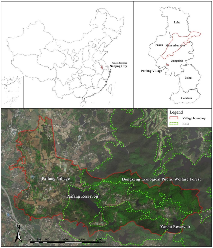
2.1. Study Area and Data Source
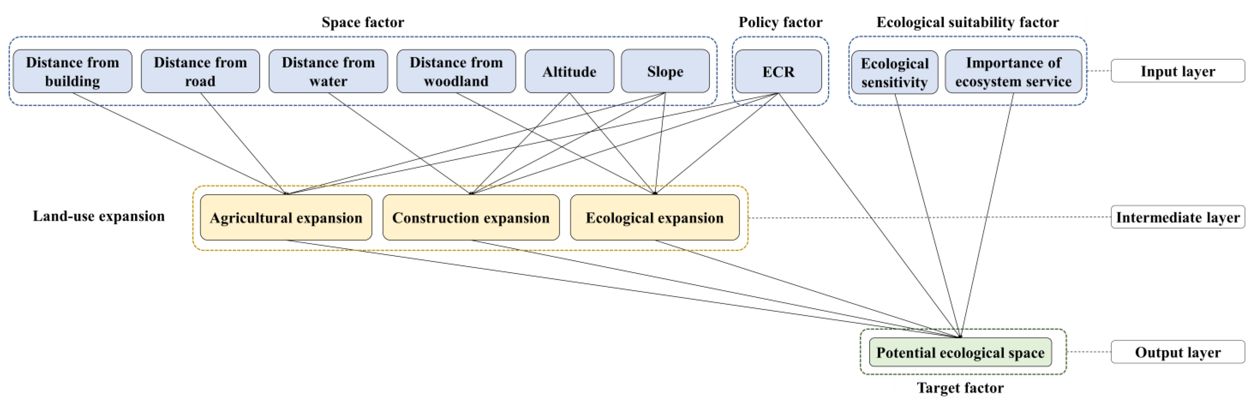
2.2. Bayesian Network Node Variable Selection
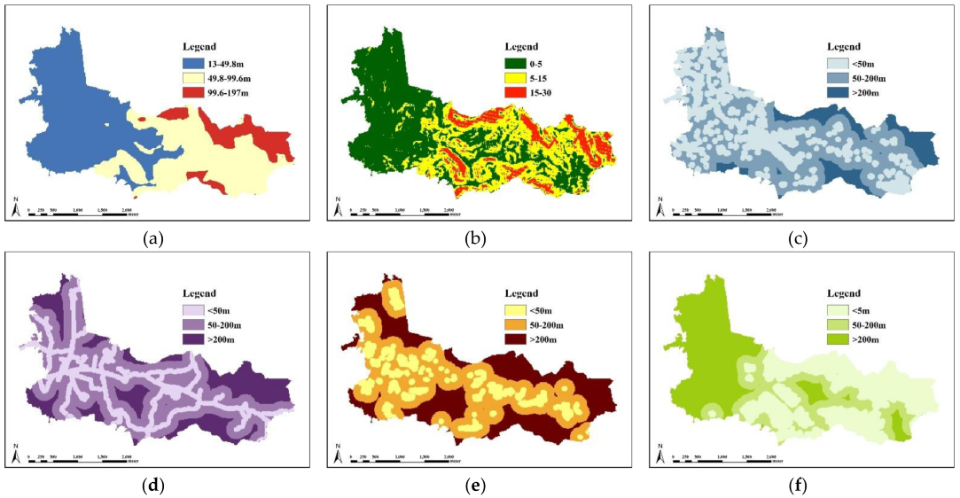
2.3. Data Processing
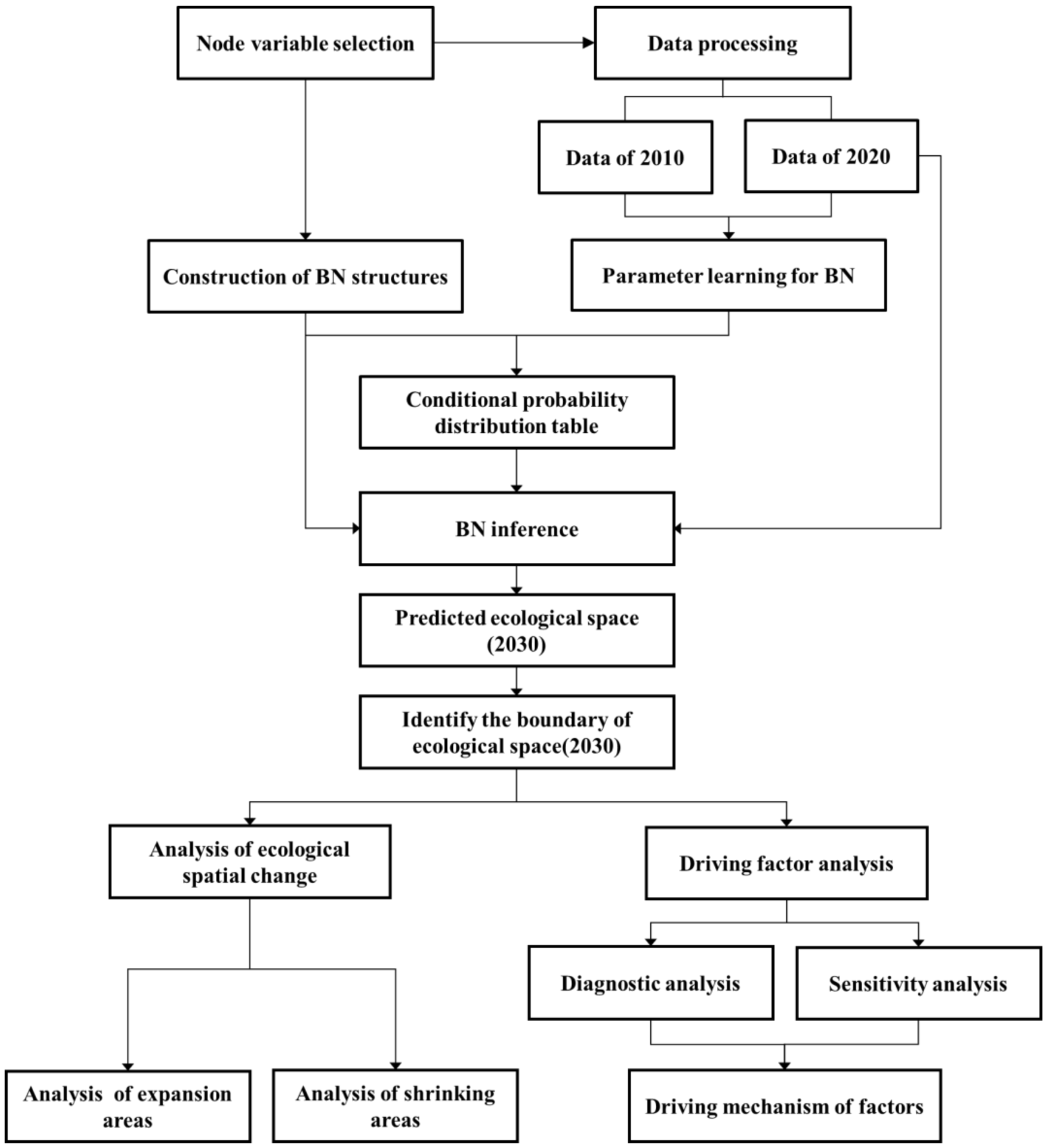
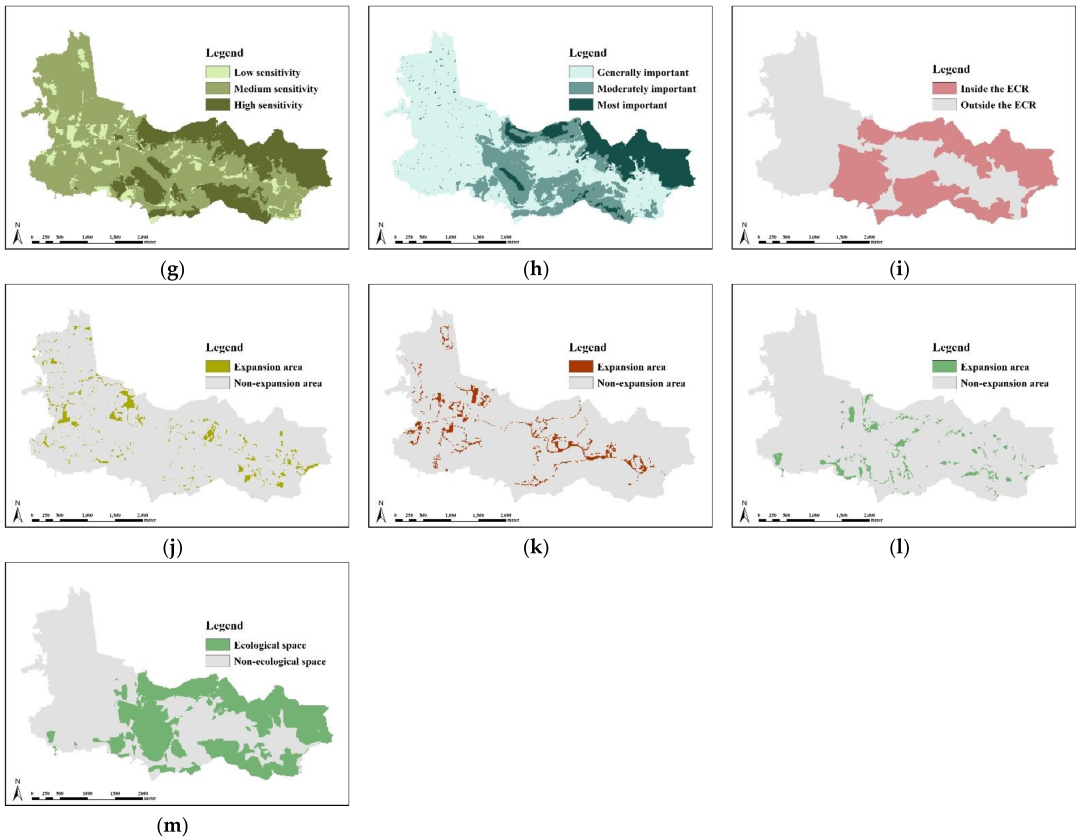
2.4. Bayesian Network Model Structuring and Parameter Learning
2.5. Bayesian Network Inference
2.6. Sensitivity and Diagnostic Analyses
3. Results
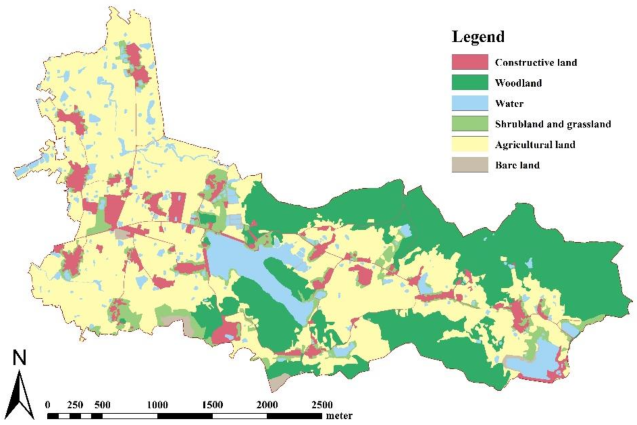
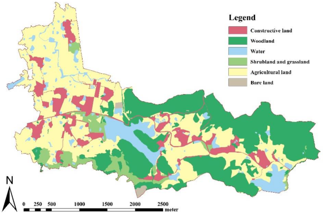
3.1. Analysis of Forecast Results
3.2. Results of Sensitivity and Diagnostic Analysis
3.2.1. Sensitivity Analysis
3.2.2. Diagnostic Analysis
4. Discussion
4.1. Changes in Ecological Space and Suggestions for Protection
4.2. Driving Factors Affecting Ecological Spatial Change and Their Mechanisms
4.3. Evolution of the Ecological Space Boundary and Its Impact
4.4. The Protective Effect of The ECR on Ecological Space
4.5. Limitations
5. Conclusions
- (1)
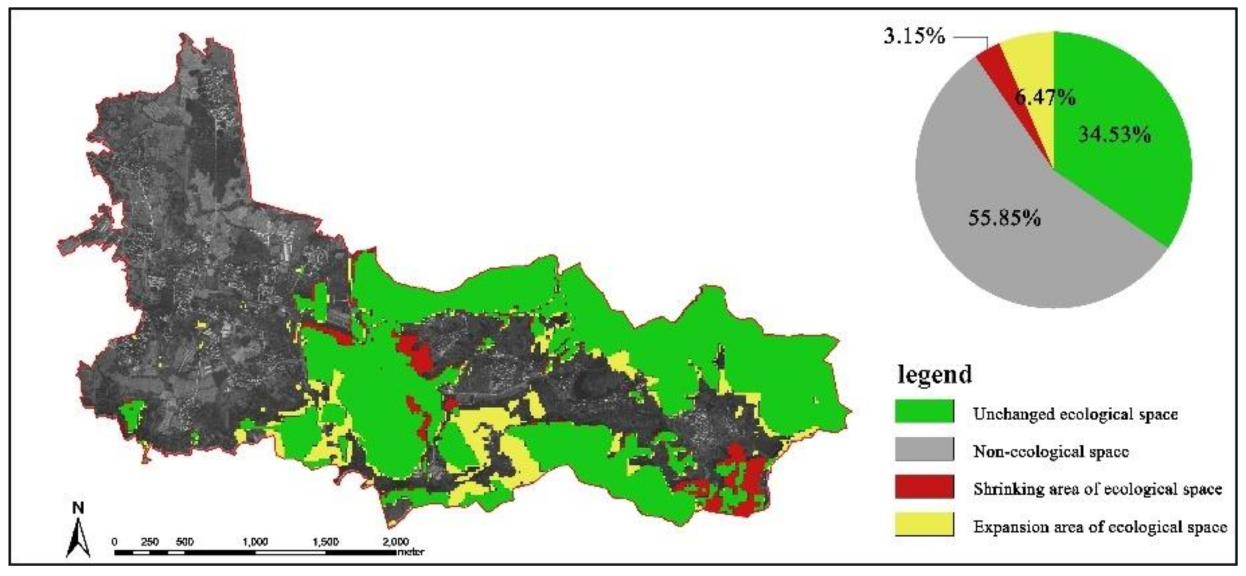
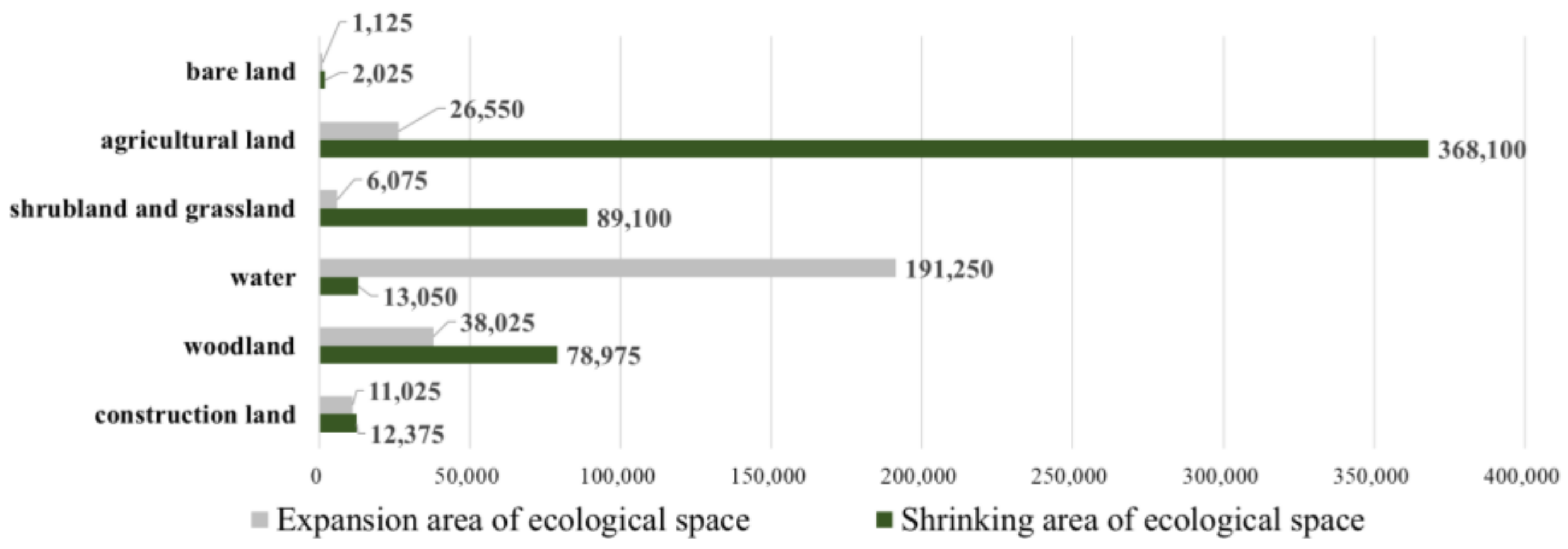
- It was predicted that the total ecological space area of Paifang Village in 2030 will be 3,587,175 m2, demonstrating expansion compared with 2020. Changes in the ecological space include expansion as well as shrinkage. Agricultural land has the greatest potential for ecological restoration, followed by shrubland and grassland, while water bodies and their surrounding areas are potential areas of shrinking ecological space that need to be focused on;
- (2)
- Competition exists between ecological and production spaces in urban fringe areas. Artificial construction activities and changes in agricultural land will disturb the ecological space to a certain extent and are the main driving factors affecting the changes in ecological space boundaries;
- (3)
- The edge of rural ecological spaces in urban fringe areas is often in an unstable state. The flow of material and energy in this type of area is relatively active and has various functional values and good recovery potential;
- (4)
- The protection effect of the ECR on the rural ecological space is remarkable. In addition to the strict protection of the area within the ECR, attention should also be paid to the protection of the ecological space outside the ECR boundary.
Author Contributions
Funding
Institutional Review Board Statement
Informed Consent Statement
Data Availability Statement
Conflicts of Interest
References
- Wang, Y.; Liu, B. CD Discussions on rural landscape and rural landscape planning in China. Chin. Landsc. Archit. 2003, 1, 55–58. [Google Scholar]
- National Bureau of Statistics. Bulletin of the Seventh National Census (No. 7)—Urban and Rural Population and Floating Population. 2021. Available online: http://www.gov.cn/xinwen/2021-05/11/content_5605791.htm (accessed on 11 May 2022).
- Commentator of Guangming Daily. Improve Rural Environment and Build Beautiful Countryside. Guangming Daily. 2018. Available online: https://news.gmw.cn/2018-02/06/content_27591798.htm (accessed on 11 May 2022).
- Huang, G. Functions, problems and countermeasures of China’s rural ecosystems. Chin. J. Eco-Agric. 2019, 27, 177–186. [Google Scholar]
- Zhao, M. A discussion on community building and community preference in city planning. Planners 2013, 29, 5–10. [Google Scholar]
- Li, K.Y.; Jin, X.L.; Ma, D.X.; Jiang, P.H. Evaluation of resource and environmental carrying capacity of China’s rapid-urbanization areas: A case study of Xinbei District, Changzhou. Land 2019, 8, 69. [Google Scholar] [CrossRef]
- Tang, C.L.; He, Y.H.; Zhou, G.H.; Zeng, S.S.; Xiao, L.Y. Optimizing the spatial organization of rural settlements based on life quality. J. Geogr. Sci. 2018, 28, 685–704. [Google Scholar] [CrossRef]
- Long, H.L.; Liu, Y.Q.; Hou, X.G.; Li, T.T.; Li, Y.R. Effects of land use transitions due to rapid urbanization on ecosystem services: Implications for urban planning in the new developing area of China. Habitat Int. 2014, 44, 536–544. [Google Scholar] [CrossRef]
- Yue, W.; Wang, T.; Zhen, Y. Unified zoning of territorial space use control derived from the core concept of “Three Types of Spatial Zones and Alert-lines”. China Land Sci. 2020, 34, 52–59+68. [Google Scholar]
- General Office of the CPC Central Committee; General Office of the State Council. Pilot Program of Provincial Spatial Planning. 2017. Available online: http://www.gov.cn/zhengce/2017-01/09/content_5158211.htm (accessed on 11 May 2022).
- Central Committee of the Communist Party of China; The State Council. Several Opinions on Establishing a Land Spatial Planning System and Supervising Its Implementation. 2019. Available online: http://www.gov.cn/zhengce/2019-05/23/content_5394187.htm (accessed on 11 May 2022).
- Huang, J.; Lin, H.; Qi, X. A literature review on optimization of spatial development pattern based on ecological-production-living space. Prog. Geogr. 2017, 36, 378–391. [Google Scholar]
- Ministry of Ecology and Environment of the People’s Republic of China. Technical Guide for Delimitation of Ecological Conservation Redline. 2017. Available online: https://www.mee.gov.cn/gkml/hbb/bgt/201707/W020170728397753220005.pdf (accessed on 11 May 2022).
- Gilman, R.; Gilman, D. Eco-Villages and Sustainable Communities: A Report for Gaia Trust by Context Institute; Context Institute: Langley, WA, USA, 1991. [Google Scholar]
- Rogers, K.S. Ecological Security and Multinational Corporation. 1997. Available online: https://www.files.ethz.ch/isn/136132/ECSP%20report_3.pdf#page=29 (accessed on 11 May 2022).
- Liu, C. Iop in research on planning and design of rural characteristic landscape from the perspective of sustainable development. In Proceedings of the 5th International Conference on Environmental Science and Material Application (ESMA), Xi’an, China, 15–16 December 2019. [Google Scholar]
- Zhao, T.Y.; Cheng, Y.N.; Fan, Y.Y.; Fan, X.N. Functional tradeoffs and feature recognition of rural production-living-ecological spaces. Land 2022, 11, 1103. [Google Scholar] [CrossRef]
- Yang, Y.Y.; Bao, W.K.; Li, Y.H.; Wang, Y.S.; Chen, Z.F. Land use transition and its eco-environmental effects in the Beijing-Tianjin-Hebei urban agglomeration: A production-living-ecological perspective. Land 2020, 9, 285. [Google Scholar] [CrossRef]
- Kong, L.Y.; Xu, X.D.; Wang, W.; Wu, J.X.; Zhang, M.Y. Comprehensive evaluation and quantitative research on the living protection of traditional villages from the perspective of “production-living-ecology”. Land 2021, 10, 570. [Google Scholar] [CrossRef]
- Bai, R.; Shi, Y.; Pan, Y. Land-use classifying and identification of the production-living-ecological space of island villages-A Case study of islands in the western sea area of Guangdong Province. Land 2022, 11, 705. [Google Scholar] [CrossRef]
- Fei, J.B.; Xia, J.G.; Hu, J.; Shu, X.Y.; Wu, X.; Li, J. Research progress of ecological space and ecological land in China. Chin. J. Eco-Agric. 2019, 27, 1626–1636. [Google Scholar]
- Demestihas, C.; Plenet, D.; Genard, M.; Raynal, C.; Lescourret, F. Ecosystem services in orchards. A review. Agron. Sustain. Dev. 2017, 37, 1–21. [Google Scholar]
- Xue, H.; Li, S.; Chang, J. Combining ecosystem service relationships and DPSIR framework to manage multiple ecosystem services. Environ. Monit. Assess. 2015, 187, 1–15. [Google Scholar] [CrossRef]
- Ministry of Natural Resources of the People’s Republic of China. National “Three Zones and Three Lines” Delineation Rules. Available online: https://www.mnr.gov.cn/dt/ywbb/202204/t20220428_2735148.html (accessed on 11 May 2022).
- Beecher. Nesting Birds and the Vegetation Substrate; Chicago Omithological Society: Chicago, IL, USA, 1942. [Google Scholar]
- Chen, J.; Wang, S.S.; Zou, Y.T. Construction of an ecological security pattern based on ecosystem sensitivity and the importance of ecological services: A case study of the Guanzhong Plain urban agglomeration, China. Ecol. Indic. 2022, 136, 108688. [Google Scholar] [CrossRef]
- Xu, X.; Tan, Y.; Yang, G.; Barnettc, J. China’s ambitious ecological red lines. Land Use Policy 2018, 79, 447–451. [Google Scholar] [CrossRef]
- Ministry of Environmental Protection of the People’s Republic of China. Technical Guide for Delineation of Ecological Conservation Redline. 2015. Available online: https://www.mee.gov.cn/gkml/hbb/bwj/201505/t20150518_301834.htm (accessed on 11 May 2022).
- Blackwell, M.S.A.; Pilgrim, E.S. Ecosystem services delivered by small-scale wetlands. Hydrol. Sci. J. 2011, 56, 1467–1484. [Google Scholar] [CrossRef]
- Stine, P.A.; Hunsaker, C.T. An Introduction to Uncertainty Issues for Spatial Data Used in Ecological Applications. In Spatial Uncertainty in Ecology; Hunsaker, C.T., Goodchild, M.F., Friedl, M.A., Case, T.J., Eds.; Springer: New York, NY, USA, 2001; pp. 91–107. [Google Scholar]
- Zhang, S.; Zhuang, Y. Relationship between ecological space and ecological conservation redline from the perspective of management requirements. Biodivers. Sci. 2022, 30, 21441. [Google Scholar] [CrossRef]
- Knaapen, J.P.; Scheffer, M.; Harms, B. Estimating habitat isolation in landscape. Landsc. Urban Plan. 1992, 23, 1–16. [Google Scholar] [CrossRef]
- Xiao, P.N.; Xu, J.; Zhao, C. Conflict identification and zoning optimization of “production-living-ecological” space. Int. J. Environ. Res. Public Health 2022, 19, 7990. [Google Scholar] [CrossRef] [PubMed]
- Mansour, S.; Al-Belushi, M.; Al-Awadhi, T. Monitoring land use and land cover changes in the mountainous cities of Oman using GIS and CA-Markov modelling techniques. Land Use Policy 2020, 91, 104414. [Google Scholar] [CrossRef]
- Xu, T.T.; Zhou, D.J.; Li, Y.H. Integrating ANNs and cellular automata-markov chain to simulate urban expansion with annual land use data. Land 2022, 11, 1074. [Google Scholar] [CrossRef]
- Pijanowski, B.C.; Tayyebi, A.; Doucette, J.; Pekin, B.K.; Braun, D.; Plourde, J. A big data urban growth simulation at a national scale: Configuring the GIS and neural network based land transformation model to run in a High Performance Computing (HPC) environment. Environ. Model. Softw. 2014, 51, 250–268. [Google Scholar] [CrossRef]
- Rahman, M.T.U.; Tabassum, F.; Rasheduzzaman, M.; Saba, H.; Sarkar, L.; Ferdous, J.; Uddin, S.Z.; Islam, A. Temporal dynamics of land use/land cover change and its prediction using CA-ANN model for southwestern coastal Bangladesh. Environ. Monit. Assess. 2017, 189, 565. [Google Scholar] [CrossRef]
- Jiang, W.G.; Chen, Z.; Lei, X.; Jia, K.; Wu, Y.F. Simulating urban land use change by incorporating an autologistic regression model into a CLUE-S model. J. Geogr. Sci. 2015, 25, 836–850. [Google Scholar] [CrossRef]
- Verburg, P.H.; Soepboer, W.; Veldkamp, A.; Limpiada, R.; Espaldon, V.; Mastura, S.S.A. Modeling the spatial dynamics of regional land use: The CLUE-S model. Environ. Manag. 2002, 30, 391–405. [Google Scholar] [CrossRef]
- Hagoort, M.; Geertman, S.; Ottens, H. Spatial externalities, neighborhood rules and CA land-use modelling. Ann. Reg. Sci. 2008, 42, 39–56. [Google Scholar] [CrossRef]
- Verburgab, P.H.; de Nijs, T.C.M.; van Eck, J.R.; Visser, H.; de Jong, K. A method to analyse neighborhood characteristic of land use patterns. Comput. Environ. Urban Syst. 2004, 28, 667–690. [Google Scholar] [CrossRef]
- Liu, X.P.; Liang, X.; Li, X.; Xu, X.C.; Ou, J.P.; Chen, Y.M.; Li, S.Y.; Wang, S.J.; Pei, F.S. A future land use simulation model (FLUS) for simulating multiple land use scenarios by coupling human and natural effects. Landsc. Urban Plan. 2017, 168, 94–116. [Google Scholar] [CrossRef]
- He, C.Y.; Okada, N.; Zhang, Q.F.; Shi, P.J.; Li, J.G. Modelling dynamic urban expansion processes incorporating a potential model with cellular automata. Landsc. Urban Plan. 2008, 86, 79–91. [Google Scholar] [CrossRef]
- Huang, Q.; Zheng, X.Q.; Liu, F.; Hu, Y.C.; Zuo, Y.Q. Dynamic analysis method to open the “black box” of urban metabolism. Resour. Conserv. Recycl. 2018, 139, 377–386. [Google Scholar] [CrossRef]
- Arsanjani, J.J.; Helbich, M.; Kainz, W.; Boloorani, A.D. Integration of logistic regression, Markov chain and cellular automata models to simulate urban expansion. Int. J. Appl. Earth Obs. Geoinf. 2013, 21, 265–275. [Google Scholar] [CrossRef]
- Wang, H.; Stephenson, S.R.; Qu, S.J. Modeling spatially non-stationary land use/cover change in the lower Connecticut River Basin by combining geographically weighted logistic regression and the CA-Markov model. Int. J. Geogr. Inf. Sci. 2019, 33, 1313–1334. [Google Scholar] [CrossRef]
- Zhang, Q. Dynamic uncertain causality graph for knowledge representation and probabilistic reasoning: Directed cyclic graph and joint probability distribution. IEEE Trans. Neural Netw. Learn. Syst. 2015, 26, 1503–1517. [Google Scholar] [CrossRef] [PubMed]
- McCloskey, J.T.; Lilieholm, R.J.; Cronan, C. Using Bayesian belief networks to identify potential compatibilities and conflicts between development and landscape conservation. Landsc. Urban Plan. 2011, 101, 190–203. [Google Scholar] [CrossRef]
- Aitkenhead, M.J.; Aalders, I.H. Predicting land cover using GIS, Bayesian and evolutionary algorithm methods. J. Environ. Manag. 2009, 90, 236–250. [Google Scholar] [CrossRef]
- Meyer, S.R.; Johnson, M.L.; Lilieholm, R.J.; Cronan, C.S. Development of a stakeholder-driven spatial modeling framework for strategic landscape planning using Bayesian networks across two urban-rural gradients in Maine, USA. Ecol. Model. 2014, 291, 42–57. [Google Scholar] [CrossRef]
- Ayre, K.K.; Landis, W.G. A Bayesian approach to landscape ecological risk assessment applied to the Upper Grande Ronde Watershed, Oregon. Hum. Ecol. Risk Assess. 2012, 18, 946–970. [Google Scholar] [CrossRef]
- Weil, K.K.; Cronan, C.S.; Meyer, S.R.; Lilieholm, R.J.; Danielson, T.J.; Tsomides, L.; Owen, D. Predicting stream vulnerability to urbanization stress with Bayesian network models. Landsc. Urban Plan. 2018, 170, 138–149. [Google Scholar] [CrossRef]
- Aalders, I. Modeling land-use decision behavior with Bayesian belief networks. Ecol. Soc. 2008, 13, 16. [Google Scholar] [CrossRef]
- Landuyt, D.; Broekx, S.; Goethals, P.L.M. Bayesian belief networks to analyse trade-offs among ecosystem services at the regional scale. Ecol. Indic. 2016, 71, 327–335. [Google Scholar] [CrossRef]
- Chen, S.H.; Pollino, C.A. Good practice in Bayesian network modelling. Environ. Model. Softw. 2012, 37, 134–145. [Google Scholar] [CrossRef]
- Frayer, J.; Sun, Z.L.; Muller, D.; Munroe, D.K.; Xu, J.C. Analyzing the drivers of tree planting in Yunnan, China, with Bayesian networks. Land Use Policy 2014, 36, 248–258. [Google Scholar] [CrossRef]
- Tian, F.H.; Li, M.Y.; Han, X.L.; Liu, H.; Mo, B.X. A production-living-ecological space model for land-use optimisation: A case study of the core Tumen River region in China. Ecol. Model. 2020, 437. [Google Scholar] [CrossRef]
- Murphy, K.P. The bayes net toolbox for Matlab. Comput. Sci. Stat. 2001, 33, 1024–1034. [Google Scholar]
- Mahjoub, M.A.; Kalti, K. Software comparison dealing with Bayesian networks. In Proceedings of the 8th International Symposium on Neural Networks, Guilin, China, 29 May–1 June 2011; pp. 168–177. [Google Scholar]
- Nanjing Municipal Bureau of Ecological Environment. Regional Protection Planning of Ecological Conservation Redline in Jiangsu Province. 2018. Available online: http://hbj.nanjing.gov.cn/hbyw/zrst/201804/t20180410_615032.html (accessed on 11 May 2022).
- Zhao, N.; Yang, Y.H.; Zhou, X.Y. Application of geographically weighted regression in estimating the effect of climate and site conditions on vegetation distribution in Haihe Catchment, China. Plant Ecol. 2010, 209, 349–359. [Google Scholar] [CrossRef]
- Schluter, M.; Savitsky, A.G.; McKinney, D.C.; Lieth, H. Optimizing long-term water allocation in the Amudarya River delta: A water management model for ecological impact assessment. Environ. Model. Softw. 2005, 20, 529–545. [Google Scholar] [CrossRef]
- Hiddink, J.G.; Jennings, S.; Kaiser, M.J. Assessing and predicting the relative ecological impacts of disturbance on habitats with different sensitivities. J. Appl. Ecol. 2007, 44, 405–413. [Google Scholar]
- Wu, J.G. Landscape sustainability science: Ecosystem services and human well-being in changing landscapes. Landsc. Ecol. 2013, 28, 999–1023. [Google Scholar] [CrossRef]
- Leemans, R.; Groot, R.S. Millennium ecosystem assessment series. In Ecosystems and Human Well-Being: A Framework for Assessmen; Island Press: Washington, DC, USA, 2003. [Google Scholar]
- Costanza, R.; de Groot, R.; Sutton, P.; van der Ploeg, S.; Anderson, S.J.; Kubiszewski, I.; Farber, S.; Turner, R.K. Changes in the global value of ecosystem services. Glob. Environ. Change-Hum. Policy Dimens. 2014, 26, 152–158. [Google Scholar] [CrossRef]
- Jin, X.; Wei, L.; Wang, Y.; Lu, Y. Construction of ecological security pattern based on the importance of ecosystem service functions and ecological sensitivity assessment: A case study in Fengxian County of Jiangsu Province, China. Environ. Dev. Sustain. 2021, 23, 563–590. [Google Scholar] [CrossRef]
- HaiWei, Y.I.N.; Xu, J.; Chen, C.; Kong, F. GIS-based ecological sensitivity analysis in the East of Wujiang City. Sci. Geogr. Sin. 2006, 26, 64–69. [Google Scholar]
- Saaty, T.L. How to make a decision—The analytic hierarchy process. Eur. J. Oper. Res. 1990, 48, 9–26. [Google Scholar] [CrossRef]
- Rao, E.; Ouyang, Z.; Yu, X.; Xiao, Y. Spatial patterns and impacts of soil conservation service in China. Geomorphology 2014, 207, 64–70. [Google Scholar] [CrossRef]
- Zeng, Z.; Piao, S.; Lin, X.; Yin, G.; Peng, S.; Ciais, P.; Myneni, R.B. Global evapotranspiration over the past three decades: Estimation based on the water balance equation combined with empirical models. Environ. Res. Lett. 2012, 7, 014026. [Google Scholar] [CrossRef]
- Renard, K.G. Predicting Soil Erosion by Water: A Guide to Conservation Planning with the Revised Universal Soil Loss Equation (RUSLE); U.S. Department of Agriculture, Agricultural Research Service: Washington, DC, USA, 2008.
- Ji, Z.W.; Xia, Q.B.; Meng, G.M. A review of parameter learning methods in Bayesian network. In Proceedings of the International Conference on Intelligent Computing ICIC 2015: Advanced Intelligent Computing Theories and Applications, Fuzhou, China, 20–23 August 2015; pp. 3–13. [Google Scholar]
- Pollino, C.A.; Woodberry, O.; Nicholson, A.; Korb, K.; Hart, B.T. Parameterisation and evaluation of a Bayesian network for use in an ecological risk assessment. Environ. Model. Softw. 2007, 22, 1140–1152. [Google Scholar] [CrossRef]
- Landuyt, D.; Broekx, S.; Engelen, G.; Uljee, I.; Van der Meulen, M.; Goethals, P.L.M. The importance of uncertainties in scenario analyses—A study on future ecosystem service delivery in Flanders. Sci. Total Environ. 2016, 553, 504–518. [Google Scholar] [CrossRef]
- Bai, L.; Xiu, C.; Feng, X.; Liu, D. Influence of urbanization on regional habitat quality:a case study of Changchun City. Habitat Int. 2019, 9, 102042. [Google Scholar] [CrossRef]
- Yeh, A.G.O.; Li, X. Economic development and agricultural land loss in the Pearl River Delta, China. Habitat Int. 1999, 23, 373–390. [Google Scholar]
- Gu, X.; Xie, B.; Zhang, Z.; Guo, H. Rural multifunction in Shanghai suburbs: Evaluation and spatial characteristics based on villages. Habitat Int. 2019, 92, 102041. [Google Scholar] [CrossRef]
- Zhou, D.; Xu, J.; Lin, Z. Conflict or coordination? Assessing land use multi-functionalization using production-living-ecology analysis. Sci. Total Environ. 2017, 577, 136–147. [Google Scholar] [CrossRef] [PubMed]
- Harris, L.D. Edge effects and conservation of biotic diversity. Conserv. Biol. 1988, 2, 330–332. [Google Scholar] [CrossRef]
- Johnston, C.A.; Pastor, J.; Pinay, G. Quantitative methods for studying landscape boundaries. In Landscape Boundaries; Ecological Studies; Hansen, A.J., di Castri, F., Eds.; Springer: New York, NY, USA, 1992; Volume 92. [Google Scholar]
- Wiens, J.A. Ecological flows across landscape boundaries: A conceptual overview. In Landscape Boundaries; Ecological Studies; Hansen, A.J., di Castri, F., Eds.; Springer: New York, NY, USA, 1992; Volume 92. [Google Scholar]
- Jiang, C.H.; Li, G.Y.; Li, H.Q.; Li, M. Iop in the study of ecological service value of farmland ecosystem in the Beijing-Tianjin-Hebei Region. In Proceedings of the International Conference on Sustainable Development on Energy and Environment Protection (SDEEP), Yichang, China, 28–30 July 2017. [Google Scholar]
- Zhao, Q.G.; Yang, J.S.; Zhou, H. “Ten words” strategic policy for ensuring red line of farmland and food security in China. Soils 2011, 43, 681–687. [Google Scholar]
- Su, S.L.; Wan, C.; Li, J.; Jin, X.F.; Pi, J.H.; Zhang, Q.W.; Weng, M. Economic benefit and ecological cost of enlarging tea cultivation in subtropical China: Characterizing the trade-off for policy implications. Land Use Policy 2017, 66, 183–195. [Google Scholar] [CrossRef]
- Zhang, C.; Lin, D.Y.; Wang, L.X.; Hao, H.G.; Li, Y.Y. The Effects of the Ecological Conservation Redline in China: A Case Study in Anji County. Int. J. Environ. Res. Public Health 2022, 19, 7701. [Google Scholar] [CrossRef]
- Li, S.; Zhu, C.; Lin, Y.; Dong, B.; Chen, B.; Si, B.; Li, Y.; Deng, X.; Gan, M.; Zhang, J.; et al. Conflicts between agricultural and ecological functions and their driving mechanisms in agroforestry ecotone areas from the perspective of land use functions. J. Clean. Prod. 2021, 317, 128453. [Google Scholar] [CrossRef]


| Variable Layer | Variable Type | Index |
|---|---|---|
| Input layer | Space factor | Altitude |
| Slope | ||
| Distance from water | ||
| Distance from roads | ||
| Distance from buildings | ||
| Distance from woodland | ||
| Ecological suitability factor | Ecological sensitivity | |
| Importance of ecosystem service | ||
| Policy factor | ECR | |
| Intermediate layer | Land-use expansion | Agricultural expansion |
| Construction expansion | ||
| Ecological expansion | ||
| Output layer | Target factor | Potential ecological space |
| Variable Type | Index | Value Type | Classification Code | ||
|---|---|---|---|---|---|
| 1 | 2 | 3 | |||
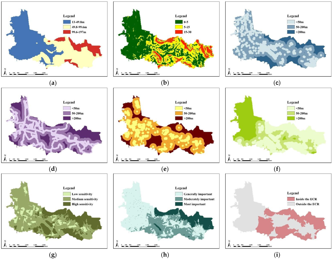
| Space factor | Altitude | Continuous | 13–49.8 m | 49.8–99.6 m | 99.6–197 m |
| Slope | Continuous | 0–5 | 5–15 | >15 | |
| Distance from water | Continuous | 0–50 m | 50–200 m | >200 m | |
| Distance from roads | Continuous | 0–50 m | 50–200 m | >200 m | |
| Distance from buildings | Continuous | 0–50 m | 50–200 m | >200 m | |
| Distance from woodland | Continuous | 0–50 m | 50–200 m | >200 m | |
| Ecological suitability factor | Ecological sensitivity | Continuous | Low sensitivity | Medium sensitivity | High sensitivity |
| Importance of ESV | Continuous | Generally important | Moderately important | Most important | |
| Policy factor | ECR | Discrete | Inside the ECR | Outside the ECR | - |
| Land-use expansion | Agricultural expansion | Discrete | Expansion area | Non-expansion area | - |
| Construction expansion | Discrete | Expansion area | Non-expansion area | - | |
| Ecological expansion | Discrete | Expansion area | Non-expansion area | - | |
| Target factor | Potential ecological space | Discrete | Ecological space | Non-ecological space | - |
| Variable Type | Index | Variance Reduction/% |
|---|---|---|
| Space factor | Altitude | 3.19 |
| Slope | 1.19 | |
| Distance from water | 0.51 | |
| Distance from roads | 0.30 | |
| Distance from buildings | 0.51 | |
| Distance from woodland | 0.00 | |
| Ecological suitability factor | Ecological sensitivity | 57.67 |
| Importance of ESV | 5.49 | |
| Policy factor | ECR | 59.56 |
| Land-use expansion | Agricultural expansion | 2.43 |
| Construction expansion | 5.07 | |
| Ecological expansion | 1.13 |
| Variable Type | Index | Variable States | Probability Change/% |
|---|---|---|---|
| Space factor | Distance from water | <50 m | −1.4 |
| 50–200 m | 0.7 | ||
| >200 m | 0.7 | ||
| Distance from roads | <50 m | −0.3 | |
| 50–200 m | 0.5 | ||
| >200 m | −0.2 | ||
| Distance from buildings | <50 m | −0.4 | |
| 50–200 m | 0.6 | ||
| >200 m | −0.2 | ||
| Distance from woodland | <50 m | −0.2 | |
| 50–200 m | 0.1 | ||
| >200 m | 0.1 | ||
| Ecological suitability factor | Ecological sensitivity | Low sensitivity | −2.5 |
| Medium sensitivity | −25.4 | ||
| High sensitivity | 27.8 | ||
| Importance of ESV | Generally important | −12.1 | |
| Moderately important | 8.4 | ||
| Most important | 3.7 | ||
| Land-use expansion | Agricultural expansion | Expansion area | −2.86 |
| Non-expansion area | 2.9 | ||
| Construction expansion | Expansion area | −5.6 | |
| Non-expansion area | 5.3 | ||
| Ecological expansion | Expansion area | 1.9 | |
| Non-expansion area | −1.9 |
Publisher’s Note: MDPI stays neutral with regard to jurisdictional claims in published maps and institutional affiliations. |
© 2022 by the authors. Licensee MDPI, Basel, Switzerland. This article is an open access article distributed under the terms and conditions of the Creative Commons Attribution (CC BY) license (https://creativecommons.org/licenses/by/4.0/).
Share and Cite
Yuan, Y.; Yang, Y.; Wang, R.; Cheng, Y. Predicting Rural Ecological Space Boundaries in the Urban Fringe Area Based on Bayesian Network: A Case Study in Nanjing, China. Land 2022, 11, 1886. https://doi.org/10.3390/land11111886
Yuan Y, Yang Y, Wang R, Cheng Y. Predicting Rural Ecological Space Boundaries in the Urban Fringe Area Based on Bayesian Network: A Case Study in Nanjing, China. Land. 2022; 11(11):1886. https://doi.org/10.3390/land11111886
Chicago/Turabian StyleYuan, Yangyang, Yuchen Yang, Ruijun Wang, and Yuning Cheng. 2022. "Predicting Rural Ecological Space Boundaries in the Urban Fringe Area Based on Bayesian Network: A Case Study in Nanjing, China" Land 11, no. 11: 1886. https://doi.org/10.3390/land11111886
APA StyleYuan, Y., Yang, Y., Wang, R., & Cheng, Y. (2022). Predicting Rural Ecological Space Boundaries in the Urban Fringe Area Based on Bayesian Network: A Case Study in Nanjing, China. Land, 11(11), 1886. https://doi.org/10.3390/land11111886