How Did the Risk of Poverty-Stricken Population Return to Poverty in the Karst Ecologically Fragile Areas Come into Being?—Evidence from China

Abstract

Eliminating poverty is the primary goal of sustainable development. China has eliminated absolute poverty in 2020, yet there is a chance that it could happen again. The poor population is mostly concentrated in ecologically fragile areas. We need to take more inclusive and effective initiatives to prevent the population in ecologically fragile areas from returning to poverty. In this study, a decision tree and logistic regression model were used to assess the risk of returning to poverty in Karst ecologically fragile areas. The data comes from 303 households in four counties in Guizhou and Guangxi. There are 12 main influencing factors identified, with the percentage of workforce numbers and loans having interactive effects. The results show that: (1) Poor resilience of livelihood assets, external shocks, and the effects of some support measures will be visible after a long period, leading to "transient" poverty and return to poverty. (2) Ecological environment management in ecologically fragile areas is very important to solve the problem of returning to poverty. (3) Appropriate loans can reduce poverty, especially when loans are used to cultivate a new excellent labor force. At the same time, it is necessary to evaluate farmers’ repayment ability reasonably and scientifically to reduce the risk of returning to poverty. The combination of ecological restoration and agricultural development is the key to solving ecological and social problems in Karst areas. Efforts should be made to improve the risk-resilience of farmers’ livelihood assets and the efficiency of livelihood assets utilization by implementing targeted support measures. This research provides a new approach to studying the mechanism of poverty recurrence, which is of great practical significance for consolidating the results of poverty eradication and realizing rural vitalization.

1. Introduction

In September 2015, the United Nations General Assembly adopted the 2030 Agenda for Sustainable Development in resolution 70/1, with eliminating poverty as the primary goal of the sustainable development goals (SDGs) [1]. It is now less than a decade before the goal of eliminating global poverty is achieved by 2030 [2]. In recent years, the number of people living in extreme poverty with a daily income of less than $1.90 per person has been steadily declining. Poverty reduction has made great progress globally [3]. Through a series of poverty reduction initiatives, China eliminated absolute poverty and regional overall poverty in 2020, which is a great innovation in the history of poverty reduction. It has provided experience in poverty reduction for other countries. From 2012 to 2020, China’s poverty rate dropped from 10.2% to 0%. According to a white paper titled ”Poverty Alleviation: China’s Experience and Contribution”, China’s poverty reduction population accounts for more than 70% of the global poverty reduction population in the same period. China has achieved the poverty reduction goal of the 2030 Agenda for Sustainable Development 10 years ahead of schedule [2]. However, about 5 million people out of poverty in China are still at risk of returning to poverty. China is supposed to pay more attention to those who may return to poverty to prevent these people from risk [4]. The “No.1 Central Document” issued by the Chinese government in 2021 proposed to set up a transition period of five years from the date of poverty alleviation, to consolidate the achievements made in poverty alleviation in coordination with the extensive drive for rural vitalization. Preventing and resolving the scale risk of returning to poverty is the goal and task of the "agriculture, countryside, and farmers" work in the current period in China. It is also the foundation to advance rural vitalization [5]. Returning to poverty has become another crucial issue after the completion of the governance of absolute poverty.

Returning to poverty means that under the influence of various internal and external factors, people who have been out of poverty have returned to poverty in terms of economic income and consumption [6]. The broad sense of returning to poverty includes both poverty-stricken people falling into poverty again and normal people falling into poverty [7]. The risk of returning to poverty is the possibility that people will fall into poverty again [8]. Vulnerability is the essence of returning to poverty. Poverty vulnerability consists of two main aspects: the shocks suffered and the ability to resist shocks [9]. Poverty-returning types can be divided into three categories according to the source of impact, including policy environment, natural environment, and self-subject. Economic and social development in poor areas is backward, and farmers lack livelihood resilience. Therefore, once farmers face external risks, they will fall into poverty again [10].

The key to consolidate the existing achievements is to prevent returning to poverty, that is, to maintain the sustainability of livelihood [11]. The study on livelihood sustainability is mainly based on livelihood capital, which can reflect the family’s livelihood status by measuring the resource endowment that families use to maintain themselves [11]. In 2000, the UK Department for International Development established a sustainable livelihood framework, which consists of vulnerability background, livelihood assets, structural and process changes, livelihood strategies, and livelihood outcomes. Livelihood capital includes five types: human capital, natural capital, material capital, financial capital, and social capital [12]. Through the livelihood capital or combination of livelihood capital they possess, farmers develop specific livelihood strategies to sustain their productive lives against various risks. When farmers’ livelihood assets are lacking, it can also lead to a return to poverty [13]. How to achieve sustainable livelihoods for the poor has become the focus of poverty reduction [14]. The research of sustainable livelihood theory on poverty mostly focuses on the micro perspective, generally starting from the family unit, to study the reasons that lead farmers to return to poverty [15]. Health status, labor skills, family size, work status, skills training, low-income insurance [16], labor force status, employment status, assets, living and education expenses, low income and insurance status [17], education year [18], etc., all have an impact on returning to poverty. Multidimensional poverty, sustainable livelihoods, and vulnerability theory have also contributed to the study.

The poverty status of the poor may be influenced not only by multidimensional factors such as household characteristics and economic characteristics but also related to multidimensional contextual factors, such as economic development [19], social development [20], ecology [21], etc. Poverty occurs as a result of both individual and contextual influences [22]. Thus, regional segmentation is useful for understanding the sources of returning to poverty [23]. The "ecologically fragile areas" are areas where ecological problems are frequent [24]. It has the characteristics of weak ecosystem resistance to disturbance, strong spatio-temporal fluctuation, obvious edge effect, and poor recovery ability [25]. Fragile ecosystems and weak economic systems cause people in these ecologically fragile areas to teeter on the edge of returning to poverty [26]. Farmers are sensitive to external shocks. The ecological environment has not been completely improved after poverty alleviation, and many other reasons lead to risk [27]. We need to formulate more inclusive and effective policies to ensure people’s living standards. Therefore, it is of great theoretical and practical significance to study the risk of poverty alleviation in ecologically fragile areas. Karst area in South China is one of the fragile ecological environment areas in China, and its regional poverty problems are representative in China and even in the world [28]. The fragile ecological environment and low productivity of Karst areas require farmers to increase their labor force to intensify land reclamation. This has caused ecological degradation and further deepened poverty, leading to the formation of a "poverty trap" which is a round of human activity, ecological degradation, and poverty [29]. Especially in southwest Karst areas, rocky desertification causes poverty significantly [30]. Rocky desertification has widened the economic gap between the rocky desertification areas and the surrounding regions and even the whole country [31]. Ecological fragility plays a decisive role in regional poverty in Karst areas [32]. Land is one of the important factors of production [33]. The quality of the land will lead to the emergence of poverty by reducing the income from agricultural production [34]. In recent years, some scholars have found that the coupling relationship between rocky desertification and poverty has changed in the new era, and the ecological environment is no longer the main factor leading to poverty in Karst areas of China [28]. The influencing factors of returning to poverty in rocky desertification areas of China in the new era need to be further identified.

The complexity of rural poverty in China and the difficulty of poverty reduction have aroused the government’s extensive concern. In rural areas, residents’ livelihood strategies are highly dependent on resources closely related to their specific places of residence, including natural resources and social resources [35]. Although there are many reasons to trigger poverty return, relevant policies and correct livelihood strategies can effectively prevent it, such as health assistance, industrial assistance [36], education assistance, labor migration policy assistance [14], and ecological assistance [37], etc. However, a study found that, especially in educational assistance, only material assistance to children cannot help them get rid of poverty, and their parents also need psychological and social support [38]. While credit and debt can have a negative impact, they can also have a positive impact in terms of reduced external constraints on farm households and increased health spending, among other things [39].

Many pieces of literature have identified the factors of returning to poverty, but there are few studies on poverty return in ecologically fragile areas. They only consider the factors of livelihood capital or external shocks. Even fewer articles consider intervention measures. The methods used in the studies are mostly linear studies, trend analysis, and correlation analysis [40]. Most of them ignore the superposition effect between factors. Bao et al. combine accident chain theory with the problem of returning to poverty [7]. They argue that returning to poverty usually undergoes a cascade of successive reactions. The mechanisms of poverty return are complex, and existing studies have yet to explore the combined effects of falling back into poverty. A logistic regression model is often used to identify influencing factors, which mainly reflects the dependence between independent variables and dependent variables. It can analyze the main effect of a single variable, but cannot reflect the interaction effect between factors [41]. The decision tree model can point out the interaction among various factors and explain whether a certain factor is meaningful in each subgroup through the tree diagram, but it cannot identify the main effect and superposition effect by itself [42].

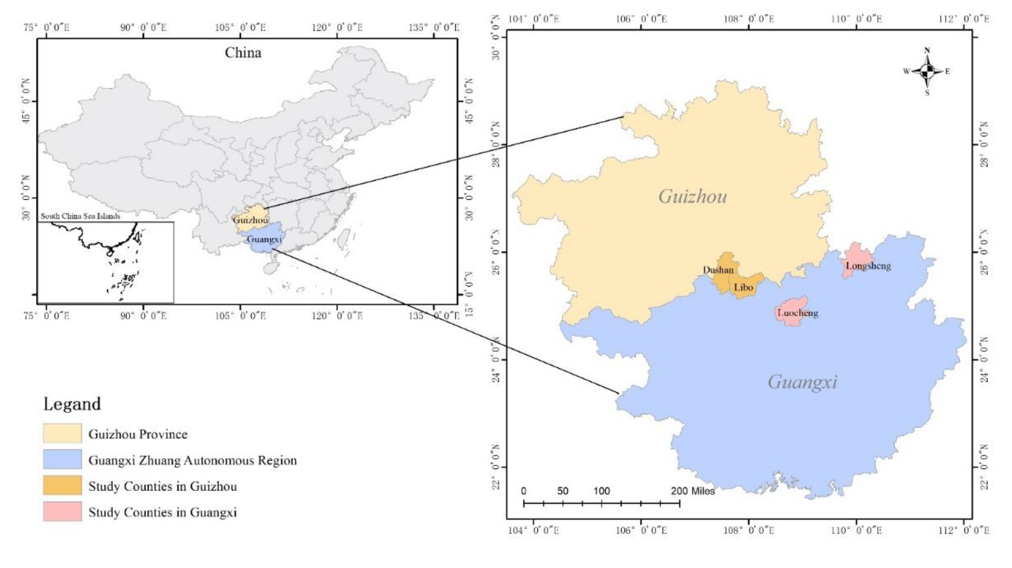
Dushan County, Libo County, Multinational Autonomous County of Longsheng, and Luocheng Mulam Autonomous County are respectively located in Guizhou Province and Guangxi Province. They are located in typical Karst rocky desertification areas, and their ecological environment is fragile. With the strong support of various policies, all four counties have been lifted out of poverty in 2020 and entered the stage of consolidating their achievements. We used a method to identify the factors specific to the risk of returning to poverty in rocky desertification ecologically fragile areas under the combination of a decision tree and logistic regression model based on research data from the four counties. As mentioned above, this study contributes to comprehensively identifying the causes of the risk of returning to poverty, as well as providing a theoretical foundation for eliminating the risk of returning to poverty in Karst’s ecologically vulnerable areas. The findings can also assist local governments in developing an early warning system for the risk of returning to poverty that is appropriate for local conditions. It can also help to accelerate the transition from consolidating poverty alleviation achievements to rural vitalization.

2. Materials and Methods

2.1. Study Area

Dushan County, Libo County, Multinational Autonomous County of Longsheng, and Luocheng Mulam Autonomous County are key ecological support counties with serious rocky desertification, which are located in the ecologically fragile areas of rocky desertification in southwest Karst mountains. They belong to typical Karst landforms. There are 48 ethnic groups living in the southwest Karst mountain area, with a population of about 100 million, including about 12 million ethnic minorities. This is the most concentrated area of poverty in China and is home to nearly 50% of the poor. These areas suffer from unfavorable factors such as poor soil, low land carrying capacity, and fragile habitats, with great population pressure and sharp contradiction between people and land [43]. The average annual temperature is above 15°C, the annual precipitation is above 1000 mm, the summer is hot and rainy, and the rain is hot at the same time, which is a typical tropical and subtropical monsoon climate [44] (Figure 1).

2.2. Data Sources

The data come from a survey conducted by the subject group from May to October 2021 in 8 townships (streets) and 32 villages in Dushan, Libo, Longsheng, and Luocheng, the key counties for ecological support. The survey used a random method to select sample farm households, trying to cover different economic conditions and different types of farm households. It was conducted through face-to-face interviews in the field to ensure the quality of the questionnaire. A total of 305 research samples were collected, of which 303 were valid. The effective rate of the sample is 99.3%, indicating that the sample is representative.

2.3. Variable Setting

This paper studies the influencing factors of the risk of returning to poverty in rocky desertification ecologically fragile areas. Based on the definition of poverty return in a broad sense, the people with the risk of returning to poverty is defined as those whose income is below the dynamic monitoring line of poverty return. Whether the poverty-stricken population has the risk of returning to poverty is set as the explained variable. In 2021, the monitoring scope of returning to poverty in Guizhou has set the monitoring object as rural households whose per capita net income is less than 6320 yuan. Therefore, according to the above criteria, if the per capita annual net income of rural households is less than 6320 yuan, there is a risk. We set the value to 1. If the per capita annual net income of rural households is more than 6320 yuan, there is no risk. We set the value to 0. Guangxi and Guizhou are adjacent to each other, and their natural, social, and economic conditions are similar. Therefore, we adopted the same standard.

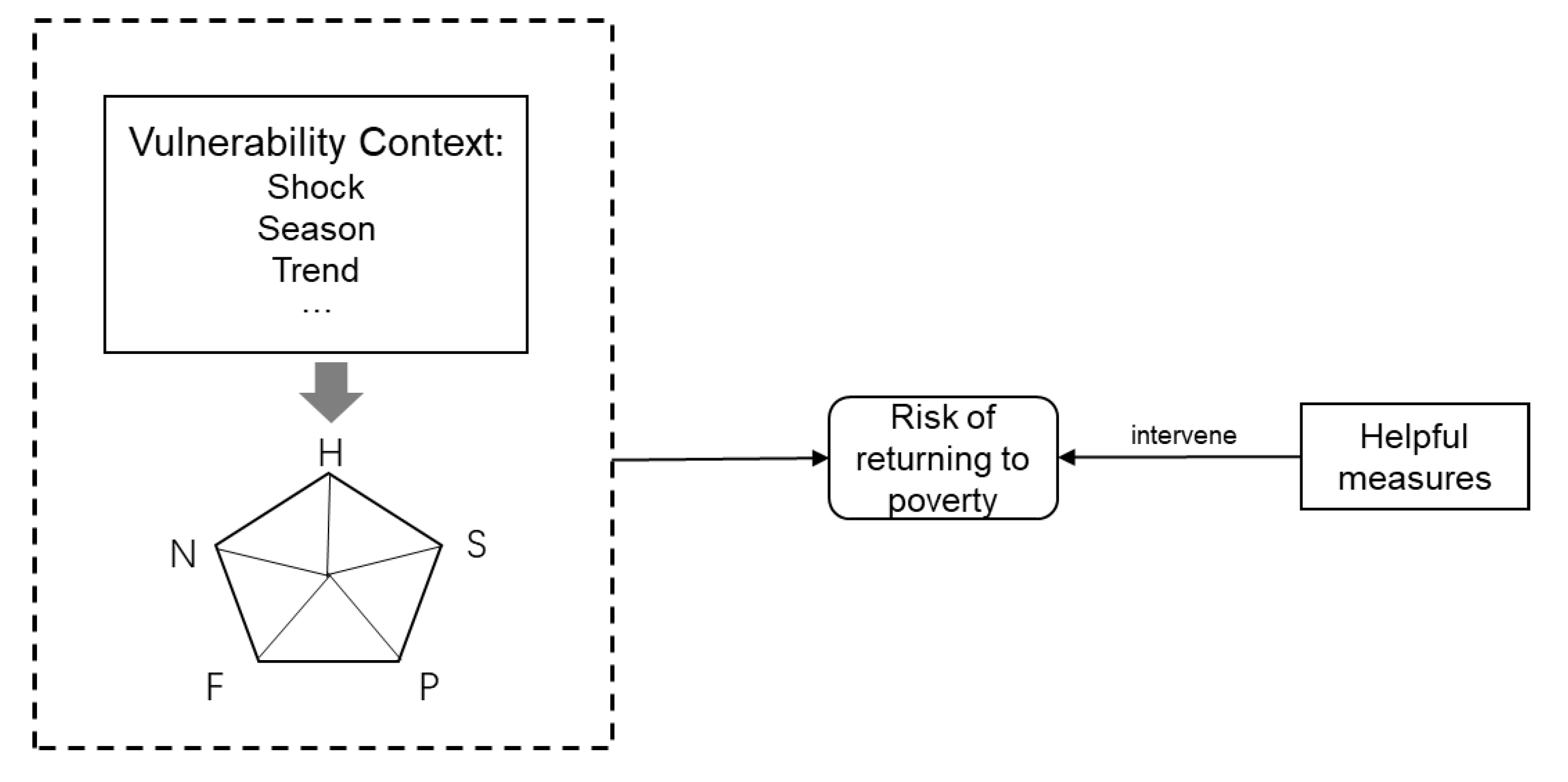
The framework of sustainable livelihood shows the core elements of livelihood and the relationship among them. In the risk environment caused by social and natural factors, farmers choose the corresponding livelihood strategies according to the nature and status of livelihood assets, which leads to a certain livelihood outcome, or it can be said whether there is a risk of returning to poverty. As a result, livelihood reacts on assets, affecting the nature and condition of assets [45]. However, in China, a series of measures have been taken to help the poor out of poverty. Besides livelihood assets, vulnerability background, and livelihood strategies, the accident chain theory holds that intervention measures that may cause "management defects" will also have an impact on the risk of returning to poverty [7]. These factors form a complex mechanism of risk of returning to poverty (Figure 2). According to the sustainable livelihood framework, we refer to the studies of Sharp [46] and Li et al. [47] and select “Average education level of labor, Workforce health status, Percentage of workforce numbers” as the influencing factors in terms of human capital; “Arable land area, Forest land area” as the influencing factors of natural capital; “Housing security situation, Housing type” as the influencing factors of physical capital; “Percentage of gift expenses, Whether to participate in farmers’ cooperatives” as social capital factors; “Whether have loans, Percentage of transfer income” as financial capital factors. Vulnerability context includes the natural environment context and the social environment context, the natural environment includes “Land degradation, Landslide, Impact of the outbreak”. The social environment includes “Percentage of education expenditures, Percentage of medical expenditures”. According to the precise poverty alleviation and support measures mentioned in the white paper "China’s Practice of Human Poverty Reduction", we selected “Industrial poverty alleviation, Ecological poverty alleviation, Health poverty alleviation, Education poverty alleviation, Outworking poverty alleviation” for the index system; these variables examine the impact of support measures on the risk of farmers returning to poverty. Industrial poverty alleviation is defined as assisting farmers in overcoming poverty by developing farming and other industries and establishing businesses. Ecological poverty alleviation aims to alleviate poverty among farmers through the implementation of ecological engineering, ecological compensation, and ecological public welfare policies. Health poverty alleviation usually refers to the implementation of serious illness medical insurance to assist farmers in getting out of poverty. Education poverty alleviation refers to subsidizing the educated children of families. Outworking poverty alleviation means that farmers can obtain the skills of migrant workers to get out of poverty through employment assistance policies. The information on the above variables is shown in

Table 1. Variable definitions and descriptive statistics.

Variable Type	Variable Name/Symbol	Variable Description and Assignment	Mean	Standard Deviation
Personal Features	Sex ($X_1$)	0 = woman; 1 = man	0.810	0.400
	Age ($X_2$)	Continuous Variables	50.350	8.830
	Nation ($X_3$)	0 = minority; 1 = Han nationality	0.170	0.372
Human Capital	Average education level of labor ($X_4$)	1 = illiterate or semi-literate; 2 = elementary school; 3 = junior high school; 4 = high school or junior college; 5 = college and above	2.775	0.587
	Workforce health status ($X_5$)	1 = disabled; 2 = with a major illness; 3 = long-term chronic illness; 4 = health	3.793	0.471
	Percentage of workforce numbers ($X_6$)	“≤0.6” =0; >0.6” =1	0.480	0.500
Natural Capital	Arable land area ($X_7$)	The total area of paddy and dry land (Acre)	5.659	5.732
	Forest land area ($X_8$)	Forest land area (Acre)	13.338	30.094
Physical Capital	Housing security situation ($X_9$)	1 = Class A; 2 = Class B; 3 = Class C; 4 = Class D	1.310	0.548
	Housing type ($X_{10}$)	1 = adobe house; 2 = mobile panel house; 3 = wooden house; 4 = brick and tile house and other brick and concrete structures; 5 = steel structure; 6 = reinforced concrete structure; 7 = other	4.040	0.749
Social Capital	Percentage of gift expenses ($X_{11}$)	Ratio of gift expenditure to total household income	0.113	0.163
	Whether to participate in farmers’ cooperatives ($X_{12}$)	1 = yes; 0 = no	0.430	0.496
Financial Capital	Whether have loans ($X_{13}$)	1 = yes; 0 = no	0.340	0.473
	Percentage of transfer income ($X_{14}$)	Ratio of transferable income to total household income	0.135	0.183
External Environmental Shocks	Land degradation ($X_{15}$)	Virtual variables, 1 = yes; 0 = no	0.120	0.324
	Landslide ($X_{16}$)	Virtual variables, 1 = yes; 0 = no	0.020	0.140
	Impact of the outbreak ($X_{17}$)	1 = no impact; 2 = low impact; 3 = average impact; 4 = high impact; 5 = very high impact	1.690	1.235
	Percentage of education expenditures ($X_{18}$)	Ratio of education expenditures to total household income	0.135	0.256
	Percentage of medical expenditures ($X_{19}$)	Ratio of medical expenditures to total household income	0.103	0.270
Measures to get out of poverty	Industrial poverty alleviation ($X_{20}$)	Virtual variables, 1 = yes; 0 = no	0.370	0.483
	Ecological poverty alleviation ($X_{21}$)	Virtual variables, 1 = yes; 0 = no	0.390	0.489
	Health poverty alleviation ($X_{22}$)	Virtual variables, 1 = yes; 0 = no	0.350	0.477
	Education poverty alleviation ($X_{23}$)	Virtual variables, 1 = yes; 0 = no	0.410	0.493
	Outworking poverty alleviation ($X_{24}$)	Virtual variables, 1 = yes; 0 = no	0.310	0.462

.

The variance inflation factor (VIF) was used to test the variables for covariance and exclude multicollinearity. It is generally believed that the VIF should not be above 5, and when the VIF is above 10, there is strong covariance among the variables. The test results show that the maximum value of VIF is 1.365, which is below 5. Therefore, there is no multicollinearity among the selected 24 independent variables.

2.4. Research Methodology

Since both a decision tree and logistic regression can be used to analyze classification problems, a statistical method is proposed to screen the interactions and analyze the linear superposition effects. The screening of the interactions is achieved through a decision tree, and then the corresponding logistic regression model is constructed and refined based on the results of the tree model to identify the main and interaction effects of the independent variables. This model can better analyze the combined effects of the influencing factors. According to Zhao et al. [48], any categorical four-gram table (

Table 2. Two groups of classification variable values definition table.

	x = 1	x = 0	Total
Y = 1	a	b	a + b
Y = 0	c	d	c + d

) can correspond to a logistic model representation $P(Y | X)\frac{exp\left({\beta }_0+{\beta }_{1}X\right)}{1+exp\left({\beta }_0+{\beta }_{1}X\right)}$, or equivalently expressed as logit(P) = ${\beta }_0$+${\beta }_1$x.

Assuming that Y is a dichotomous variable, we first performed a stratified statistical analysis using a decision tree. The statistical tests for each stratum should be significant. A decision tree was applied to identify potential interactions and then create a combination of variables. The logistic regression model was constructed based on the results of the decision tree. The decision tree was used to determine the potential interactions between the variables. According to the order of the interaction terms in the model, statistical tests were run from highest to lowest order, and the high-order interactions that were not significant were removed. Then, we added the lower-order interactions and main effects that needed to be nested and tested each item from higher-order to main effects again to build a complete logistic model [48]. The final logistic regression model presented the main effects of individual factors and the interaction effects of multiple factors.

In this study, we use scikit-learn, which is a Python module integrating a wide range of state-of-the-art machine learning algorithms to construct a decision tree model by using the CART algorithm. After growing the tree to full depth until the stopping criterion is reached, nodes providing less additional information are removed and the tree is pruned to face downwards. The CART model uses the ten-times cross-validation method and pruning techniques to minimize the mean of the root-mean-square prediction error and improve the stability of the model. We consider the model prediction good when the model prediction accuracy exceeds 70% [49].

Entropy is the basis for decision tree formation. Minimizing entropy can realize the hierarchy of decision trees. Entropy is a measure of the uncertainty of a random variable; if the uncertainty of the variable is higher, the entropy value is higher; if the variable is more stable, the entropy value is lower [50]. In decision tree classification tasks, we usually hope that the entropy value of the classified variables is low, which means the purity of the classification effect is high. The degree of entropy reduction is measured by the information gain. In building a decision tree, two features are selected for traversal, and the feature with the largest information gain is selected by calculating the entropy value, and this feature is prioritized as the node of the decision tree. This process continues until the final decision tree is formed [51].

Some parameters are used to control the depth of the tree and thus reduce overfitting. They are set as follows: max_depth, which represents the longest path between the root and leaf nodes, is 3; and the minimum number of samples required for leaf nodes (min_samples_leaf) is 10, for splitting internal nodes (min_samples_split) is 15. The standard parameters define the function used to measure the quality of the segmentation [52]. We use 70% of the sampled data as training data and the rest data for validation(test).

We use SPSS26.0 to establish the final logistic regression model as follows:

$$Y_i=\ln \left(\frac{p_i}{1-p_i}\right)={\beta }_0+{\beta }_1{X}_1+\cdots +{\beta }_j{X}_j+{\beta }_{j+1}{C}_1+\cdots +{\beta }_{j+n}{C}_n+{\epsilon }_i$$

(1)

In Formula (1), $p_i$ is the probability of people returning to poverty, 1 − $p_i$ is the probability of people not returning to poverty. $Y_i$ is the explained variable, which is the logarithm of odds. $X_1$, $X_2$, ⋯⋯$X_j$, $C_1$, $C_2$, ⋯⋯, $C_n$are explanatory variables. $C_n$ is the product of multiple $X_j$ (At least two) combined to represent the interaction term. ${\beta }_0$ is the intercept, which is a constant term. ${\beta }_1$, ${\beta }_2$, ⋯⋯, ${\beta }_{j+n}$, are regression coefficients, indicating the size of the influencing factors. ${\epsilon }_i$ is the error term. The values of i, j, and n are 1, 2, 3⋯⋯.

3. Results

3.1. Transmission and Interruption of the Risk of Returning to Poverty

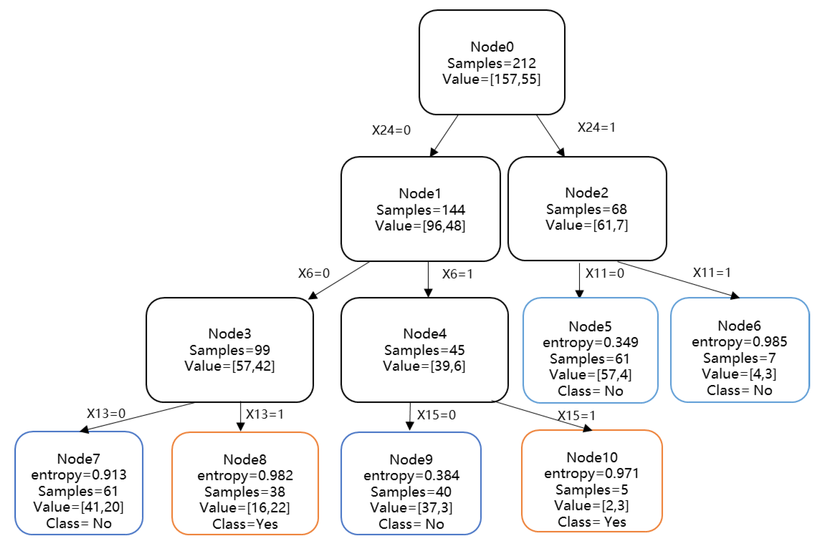
The decision tree model is used to fit the above data to obtain the corresponding decision tree results as shown in Figure 3.

The results of the decision tree in Figure 3 show several sets of classification criteria, of which the following two sets are judged to be at risk of returning to poverty:

Class 1: if Outworking poverty alleviation ($X_{24}$) = 0, Percentage of workforce numbers ($X_6$) = 0, Whether have loans ($X_{13}$) = 0, Risk of poverty returning = No;

Class 2: if Outworking poverty alleviation ($X_{24}$) = 0, Percentage of workforce numbers ($X_6$) = 0, Whether have loans ($X_{13}$) = 1, Risk of poverty returning = Yes;

Class 3: if Outworking poverty alleviation ($X_{24}$) = 0, Percentage of workforce numbers ($X_6$) = 1, Land degradation($X_{15}$) = 0, Risk of poverty returning = No;

Class 4: if Outworking poverty alleviation ($X_{24}$) = 0, Percentage of workforce numbers ($X_6$) = 1, Land degradation($X_{15}$) = 1, Risk of poverty returning = Yes;

Class 5: if Outworking poverty alleviation ($X_{24}$) = 1, Percentage of gift expenses ($X_{11}$) = 0, Risk of poverty returning = No;

Class 6: if Outworking out of poverty ($X_{24}$) = 1, Percentage of gift expenses ($X_{11}$) = 1, Risk of poverty returning = No;

(1) Loans for households who are not migrant workers out of poverty and have a low proportion of the labor force will easily lead to poverty return. Among them, the key to returning to poverty is: first, the function of going out to work to block the return to poverty has not been brought into play; second, the low percentage of workforce numbers and the superposition of loans have aggravated the return to poverty.

(2) If households do not get out of poverty by outworking, and the proportion of the labor force is high, the phenomenon of land degradation will lead to the risk of households returning to poverty. The fact that farmers did not get out of poverty by outworking indicates that farmers’ families mainly rely on local resources to get out of poverty. In essence, they still rely heavily on land for their livelihood. If land degradation occurs at this time, it will greatly affect the quality of cultivated land and the normal livelihood of farmers.

(3) The percentage of gift expenditure is an important factor. A high percentage of gift expenditure may lead to poverty return, but going out to work can effectively resist the temporary return to poverty caused by the increase of gift expenditure.

3.2. Measurement of the Main and Interaction Effects

According to the method provided in 2.4, the formula and results we calculated are as follows:

Starting from the root of the tree (Node0), a four-grid table is formed by Node1 and Node2, and the classification relationship between Y and $X_{24}$ is as follows:

$$Y={\beta }_{240}+{\beta }_{241}{X}_{24}$$

(2)

When $X_{24}$ = 1, a four-grid table is formed by Node5 and Node6, and the classification relationship between Y and $X_{24}$, $X_{11}$ ($X_{24}$ = 1) can be expressed as follows:

$$Y={\beta }_{240}+{\beta }_{241}{X}_{24}+X_{24}\left({\beta }_{110}+{\beta }_{111}{X}_{11}\right)$$

(3)

When $X_{24}$ = 0, a four-grid table is formed by Node3 and Node4, and the classification relationship between Y and $X_{24}$, $X_{11}$ ($X_{24}$ = 1), $X_6$($X_{24}=0$) can be expressed as follows:

$$Y={\beta }_{240}+{\beta }_{241}{X}_{24}+X_{24}\left({\beta }_{110}+{\beta }_{111}{X}_{11}\right)+\left(1-X_{24}\right)\left({\beta }_{60}+{\beta }_{61}{X}_6\right)$$

(4)

When $X_{24}$ = 0 and $X_6$ = 0, a four-grid table is formed by Node7 and Node8, and the classification relationship between Y and $X_{24}$, $X_{11}$ ($X_{24}$ = 1), $X_6$($X_{24}=0$), $X_{13}$($X_{24}=0,X_6=0$) can be expressed as follows:

$$Y={\beta }_{240}+{\beta }_{241}{X}_{24}+X_{24}\left({\beta }_{120}+{\beta }_{121}{X}_{12}\right)+\left(1-X_{24}\right)\left[\begin{array}{c}({\beta }_{60}+{\beta }_{61}{X}_6+\left(1-X_6\right)\\ \left({\beta }_{130}+{\beta }_{131}{X}_{13}\right)\end{array}\right]$$

(5)

When $X_{24}$ = 0 and $X_6$ = 1, a four-grid table is formed by Node9 and Node10, and the classification relationship between Y and $X_{24}$, $X_{11}$ ($X_{24}$ = 1), $X_6$($X_{24}=0$), $X_{13}$($X_{24}=0,X_6=0$), $X_{15}$($X_{24}=0,X_6=1$) can be expressed as follows:

$$Y={\beta }_{240}+{\beta }_{241}{X}_{24}+X_{24}\left({\beta }_{110}+{\beta }_{111}{X}_{11}\right)+\left(1-X_{24}\right)\left[\begin{array}{c}({\beta }_{60}+{\beta }_{61}{X}_6+\left(1-X_6\right)\left({\beta }_{130}+{\beta }_{131}{X}_{13}\right)\\ +{\beta }_{62}{X}_6\left({\beta }_{150}+{\beta }_{151}{X}_{15}\right)\end{array}\right]$$

(6)

Sort out the above expressions, and recombine the independent variables and the product of independent variables to define the regression coefficient, and obtain the following expression:

$$Y={\beta }_0+{\beta }_1{X}_{24}+{\beta }_2{X}_6+{\beta }_3{X}_{13}+{\beta }_4{X}_6{X}_{13}+{\beta }_5{X}_6{X}_{15}+{\beta }_6{X}_{24}{X}_{13}+{\beta }_7{X}_{24}{X}_6+{\beta }_8{X}_{24}{X}_{11}+{\beta }_9{X}_{24}{X}_6{X}_{13}+{\beta }_{10}{X}_{24}{X}_6{X}_{15}$$

(7)

Fit the data according to the last logistic expression after sorting out the above, eliminate items without statistical significance, and supplement the main effect items if there are interactive items but no main effect items, and test the corresponding regression coefficients. The details are shown in

Table 3. Test interaction terms with logistic models on the results of decision trees.

Variable Name	Constants	${\mathit{X}}_6$	${\mathit{X}}_{13}$	${\mathit{X}}_{24}$	${\mathit{X}}_6*{\mathit{X}}_{13}$	${\mathit{X}}_6*{\mathit{X}}_{15}$	${\mathit{X}}_{24}*{\mathit{X}}_6$	${\mathit{X}}_{24}*{\mathit{X}}_{13}$	${\mathit{X}}_{24}*{\mathit{X}}_{11}$	${\mathit{X}}_{24}*{\mathit{X}}_6*{\mathit{X}}_{13}$	${\mathit{X}}_{24}*{\mathit{X}}_6*{\mathit{X}}_{15}$	Description
Step 1												Using the results of the tree model, the corresponding logistic model was constructed, and the highest number of terms, p > 0.1, was excluded.
Regression coefficient	−0.780	−0.768	1.330	−1.981	−1.554	0.952	−0.316	−1.521	5.647	2.722	−19.064
p	0.002	0.062	0.001	0.009	0.031	0.215	0.784	0.156	0.006	0.141	0.999
Step 2												The highest number of secondary terms, $X_6*X_{15}$, $X_{24}*X_6$ and $X_{24}*X_{13}$, were excluded because they had p > 0.1.
Regression coefficient	−0.736	−0.866	1.105	−2.77	−1.172	0.847	0.717	−0.768	5.773	-	-
p	0.254	0.034	0.004	<.001	0.076	0.258	0.43	0.412	0.009	-	-
Step 3												The secondary term p < 0.1, need not be excluded. Linear superimposed variables were added.
Regression coefficient	−0.713	0.736	1.216	−2.322	−1.209	-	-		5.95	-	-
p	0.004	0.051	0.003	0.004	0.071	-	-		0.005	-	-

Note: α = 0.1, the parameter is significant at the level of p < 0.1.

.

In step 4, the two interaction items and 24 independent variables screened out in step 3 are incorporated into the Logistic model, the results are shown in

Table 4. Test interaction terms with logistic models on the results of decision trees -Step 4.

Variable	B	ST	Wald	p	OR
Sex ($X_1$)	0.947	0.570	2.764	0.196	2.579
Age ($X_2$)	0.050	0.023	4.726	0.130	0.951
Nation ($X_3$)	0.112	0.519	0.046	0.830	1.118
Average education level of labor ($X_4$)	0.379	0.332	1.306	0.253	1.461
Workforce health status ($X_5$)	−1.182	0.585	4.084	0.043 **	0.307
Percentage of workforce numbers ($X_6$)	−0.008	0.499	0.000	0.988	0.993
Arable land area ($X_7$)	0.003	0.035	0.006	0.941	1.003
Forest land area ($X_8$)	−0.001	0.007	0.030	0.863	0.999
Housing security situation ($X_9$)	−0.012	0.358	0.001	0.974	0.988
Housing type ($X_{10}$)	0.109	0.286	0.144	0.704	1.115
Percentage of gift expenses ($X_{11}$)	6.227	1.466	18.048	0.000 ***	506.342
Whether to participate in farmers’ cooperatives ($X_{12}$)	0.472	0.444	1.132	0.287	1.603
Whether have loans ($X_{13}$)	1.195	0.529	5.111	0.024 **	3.304
Percentage of transfer income ($X_{14}$)	2.202	1.108	3.951	0.047 **	9.045
Land degradation ($X_{15}$)	1.748	0.556	9.874	0.002 ***	5.743
Landslide ($X_{16}$)	3.680	1.458	6.371	0.012**	39.632
Impact of the outbreak ($X_{17}$)	−0.120	0.229	0.272	0.602	0.887
Percentage of education spending ($X_{18}$)	1.379	0.729	3.581	0.058 *	3.971
Percentage of medical expenses ($X_{19}$)	3.759	1.234	9.278	0.002 ***	42.911
Industrial poverty alleviation ($X_{20}$)	−0.879	0.466	3.561	0.059 *	0.415
Ecological poverty alleviation ($X_{21}$)	−0.444	0.427	1.081	0.298	0.641
Health poverty alleviation ($X_{22}$)	−1.095	0.641	2.921	0.087 *	0.334
Education for poverty alleviation ($X_{23}$)	0.964	0.458	4.434	0.035 **	2.623
Outworking out of poverty ($X_{24}$)	−2.019	0.558	13.100	0.000 ***	0.133
Percentage of workforce numbers * Whether have loans ($X_6{X}_{13}$)	−1.912	0.909	4.421	0.035 **	0.148
Outworking out of poverty * Percentage of gift expenses ($X_{24}{X}_{11}$)	5.530	3.462	2.552	0.110	252.221
Constants	−6.223	3.146	3.913	0.048	0.002

*, **, and *** represent significance levels of 10%, 5%, and 1%, respectively, and the values in parentheses are t values calculated with robust standard errors.

. The significant items are identified to obtain the final logistic model as follows:

$$Y=-6.223-1.182X_5+6.227X_{11}+1.195X_{13}+2.202X_{14}+1.748X_{15}+3.68X_{16}+1.379X_{18}+3.759X_{19}-0.879X_{20}-1.095X_{22}+0.964X_{23}-2.019X_{24}-1.912X_6{X}_{13}$$

(8)

In the logistic regression model, the likelihood ratio is used to test the irrelevant hypothesis, and the likelihood ratio statistics approximately obey the χ2 distribution. The −2 log-likelihood of this model is 196.613; Cox and Snell R² is 0.375; Nagelkerke R² is 0.557. The likelihood ratio chi-square value is 142.505, and the p-value is 0.000. Therefore, the model is overall significant and has good interpretability. The prediction accuracy of the model is 86.8%, and the prediction effect is good.

3.2.1. Main Effect of Variables

Workforce health status ($X_5$), Percentage of gift expenses ($X_{11}$), Whether have loans ($X_{13}$), Percentage of transfer income ($X_{14}$), Land degradation($X_{15}$), Landslide($X_{16}$), Percentage of education spending($X_{18}$), Percentage of medical expenses ($X_{19}$), Industrial poverty alleviation ($X_{20}$), Health poverty alleviation ($X_{22}$), Education for poverty alleviation ($X_{23}$), Outworking out of poverty ($X_{24}$), these variables were significant at the 0.1 level of significance and were associated with return to poverty. Additionally, Percentage of gift expenses ($X_{11}$), Whether have loans ($X_{13}$), Percentage of transfer income ($X_{14}$), Land degradation($X_{15}$), Landslide($X_{16}$), Percentage of education spending($X_{18}$), Percentage of medical expenses ($X_{19}$), Education for poverty alleviation ($X_{23}$), the coefficients of these variables are positive, because OR > 1. The occurrence of these variables when they are 1 will increase the probability of returning to poverty. Workforce health status ($X_5$), Industrial poverty alleviation ($X_{20}$), Health poverty alleviation ($X_{22}$), Outworking out of poverty ($X_{24}$), the coefficients of these variables are negative, because OR < 1. When these variables are 1, the probability of returning to poverty will be reduced. These variables reflect the main effects of returning to poverty.

3.2.2. Percentage of Workforce Numbers ($X_6$) and Whether Have Loans ($X_{13}$) have an Interactive Effect

(1) When loans are available, a higher percentage of the workforce numbers will reduce the probability of returning to poverty.

Since the percentage of the workforce numbers($X_6$)has only interaction without main effect, and it is meaningless when $X_{13}$ = 0, we only consider the case with loans. For the presence of loans, $X_{13}$ = 1 is substituted into the model to obtain.

$$\mathrm{logit}P=-5.028-1.182X_5+6.227X_{11}+2.202X_{14}+1.748X_{15}+3.68X_{16}+1.379X_{18}+3.759X_{19}-0.879X_{20}-1.095X_{21}+0.964X_{23}-2.019X_{24}-1.912X_6$$

(9)

OR = exp(−1.912) ≈ 0.148

(10)

By checking whether the sum of the regression coefficient ${\mathrm{b}}_6$ of $X_6$ and the coefficient ${\mathrm{b}}_{613}$ of $X_6{X}_{13}$ is 0, we can judge whether the interaction term $X_6{X}_{13}$ really exists. It can be seen from (9) that the sum is −1.912, not 0, and the interaction term exists. For those who have loans, it can be considered that the percentage of the workforce numbers is related to returning to poverty. From OR < 1 (10), it can be seen that the low percentage of the workforce numbers will increase the chance of returning to poverty, and from the interaction terms ${\beta }_{613}$ < 0 and P < 0.001, it can be considered that the probability of returning to poverty is greatly reduced when the percentage of the workforce numbers is high.

(2) When the percentage of the workforce numbers is low, having loans aggravates the risk of returning to poverty.

For variable loan situations ($X_{13}$), due to the interaction, it is necessary to discuss separately according to the percentage of the workforce numbers:

For people with a low percentage of the workforce numbers, $X_6$ = 0 is substituted into the model to get:

$$\mathrm{logit}P=-6.223-1.182X_5+6.227X_{11}+1.195X_{13}+2.202X_{14}+1.748X_{15}+3.68X_{16}+1.379X_{18}+3.759X_{19}-0.879X_{20}-1.095X_{22}+0.964X_{23}-2.019X_{24}$$

(11)

OR = exp(1.195) ≈ 3.304

(12)

Therefore, when the percentage of the workforce numbers is not high, whether loans are related to returning to poverty. From OR > 1 (12), it can be seen that the probability of people with a low percentage of the workforce numbers with loans returning to poverty is higher than those without loans and a low percentage of the workforce numbers.

For people with a high percentage of the workforce numbers, $X_6$ = 1 is substituted into the model to obtain:

$$\mathrm{logit}P=-6.223-1.182X_5+6.227X_{11}+0.083X_{13}+2.202X_{14}+1.748X_{15}+3.68X_{16}+1.379X_{18}+3.759X_{19}-0.879X_{20}-1.095X_{22}+0.964X_{23}-2.019X_{24}$$

(13)

OR = exp(0.083) ≈ 1.087

(14)

By checking whether the sum of the regression coefficient ${\mathrm{b}}_{13}$ of $X_{13}$ and regression coefficient ${\mathrm{b}}_{613}$ of $X_6{X}_{13}$ is 0, it can be judged whether the interaction term $X_6{X}_{13}$ really exists. It can be seen from (13) that the sum is 0.083, not 0, and the interaction term exists. For people with a high percentage of the workforce numbers, it can be considered whether loans are related to returning to poverty. From OR > 1(14), it can be seen that when the percentage of the workforce numbers is high, the chances of returning to poverty will be increased if there is a loan, and from the interaction terms ${\beta }_{613}$ < 0 and P < 0.001, it can be considered that the probability of returning to poverty will be increased when the percentage of the workforce numbers is high and there is a loan.

The test shows that the interaction of$X_6{X}_{13}$ is significant at the level of P < 0.1. At the same time, in the decision tree results in Class1 and Class2, the interaction effect arising from the overlay of the number of labor force shares and loans plays the largest role.

3.3. Livelihood Status and Returning to Poverty

Among human capital, the quality and quantity of the workforce are important factors affecting poverty return, and quality is more important than quantity in affecting poverty return. Workforce health status is a significant factor that negatively affects poverty return, reflecting the quality of the workforce, indicating that the healthier the workforce is the less likely the household will return to poverty. There is no main effect on the percentage of workforce numbers, but there is an interaction effect with loans, which has a negative effect on poverty return. More workforce quantity can reduce the shock from poverty return.

The role of social capital in resisting risks is not fully played. The share of gift expenditure is a factor that positively affects poverty return, and the higher the share of gift expenditure, the more likely to return to poverty. Chinese people are hospitable, thus mutual support and co-development is a common phenomenon. The development of rural household livelihoods is deeply influenced by the government, community, relatives and friends, and various other levels of organizations [11]. Short-term larger gift expenditures cause farmers to temporarily return to poverty, but at the same time, when further gift expenditures occur, they also establish or consolidate farmers’ external social networks accordingly, which can improve risk resistance in the long term. However, the expenditure on gifts also brings a significant financial burden, which is also related to some bad customs and habits in rural China [53]. Cooperatives, as an external mechanism in social capital, can withstand risk, but this factor is not significant. The occurrence of this phenomenon may be related to the low development of rural social organizations and the poor enthusiasm of farmers to participate in social activities in the study areas. This makes the poor people create living space inefficiently and makes them vulnerable to risks.

Loans and the percentage of transfer income in financial capital are significant factors influencing the poverty return. Interviews in this study revealed that children’s education, investment in developing industries, medical care, car purchase, and failure to start a business led to farmers’ debt. Meanwhile, the percentage of transfer income is also a significant factor affecting poverty return. The higher the percentage of transfer income represents the stronger dependence on government subsidies, and the simpler the family income structure is, the more likely to return to poverty away from policy subsidies.

3.4. External Shock and Returning to Poverty

Natural environmental shocks are more likely to cause farmers to return to poverty than social environmental shocks. In the column of external environmental impacts, natural disaster shocks have a deep impact on the occurrence of poverty return, with land degradation and landslides being important factors that significantly affect poverty return. Both also reflect the poor quality of land under natural disaster shocks. The cultivated land area and forest area are not significant, and the quality of land has a greater impact on farmers’ return to poverty than the quantity of land. Ecological key counties are located in typical rocky desertification areas, and the phenomenon of rocky desertification still exists. If the problem of rocky desertification still exists, even if the amount of land is more, it will not be beneficial to farmers. To eradicate poverty in key counties with ecological assistance, ecological projects such as comprehensive control of rocky desertification and continuous ecological assistance are needed at the source. Moreover, natural environmental factors have a greater impact on poverty return than social environmental factors, such as the COVID-19 epidemic in public health emergencies. In this study, the impact of the epidemic is not significant, which is also related to the buffering effect of the agricultural sector, which makes the labor force regain employment opportunities in rural areas, thus stabilizing the income level of the labor force and reducing the risk of returning to poverty [54].

3.5. Measures to Get out of Poverty and Returning to Poverty

Health poverty alleviation, industrial poverty alleviation, outworking poverty alleviation, and education poverty alleviation are the significant factors that affect the return to poverty. Except education poverty alleviation, other measures have a negative impact on the return to poverty and have a blocking effect on the formation of poverty return. Education poverty alleviation has a positive impact in this study, which may also be related to the particularity targeted population and the measures themselves. Education is the investment of human capital, and poverty alleviation through education has promoted this kind of investment, making ends meet in the short term, but it is still a powerful measure to reduce poverty in the long run. Outworking attracts more farmers to participate in employment, creating direct economic benefits for farmers. The hematopoietic assistance of industry poverty alleviation is manifested in developing the ecological poverty alleviation industry and bringing economic income to farmers through interest linkage and share dividends. In the new era, local governments should also focus on developing various local industries, rather than relying too much on natural resources [28]. This can essentially stimulate the endogenous motivation of farmers.

4. Discussion

This study combines decision tree and logistic regression models to jointly analyze the factors influencing the risk of returning to poverty in rocky desertification ecologically fragile areas. The combination of decision tree and logistic regression was used to identify both the main effects and interaction effects of the influencing factors, which provides a more accurate and effective method for the investigation of the mechanism of poverty return. Unlike previous studies on the influencing factors in general areas, land degradation and landslides are factors specific to Karst ecologically fragile areas.

(1) Poor livelihood resilience, external shocks, and the fact that the effects of some support measures can only be seen in the long term make farmers vulnerable to “transient” poverty.

Through a series of support measures, farmers’ livelihood holdings and capital utilization efficiency have improved. However, there are still shortcomings. Especially in the case of major events or external environmental shocks, which can expose them to the risk of returning to poverty. Although the series of support measures have been effective in accomplishing the task of eradicating absolute poverty, the effects of some measures need to be implemented over a longer period before the essential effects can be seen.

For example, forest land area in farmers’ natural capital negatively affects poverty return, but not significantly. The impact of land degradation and landslides makes farmers who are more dependent on their land more vulnerable to poverty return. Both of them make households’ land less available to resist the effects of natural capital and trap them in a cycle of poverty. A series of ecological assistance measures have been implemented in China to control this fragile ecological environment, or to help farmers get rid of the existing harsh environment. A study has analyzed many years of data and found that natural factors are no longer the most important factor affecting the return to poverty after ecological assistance improves the environment [28]. However, ecological support was not significant in this study, which is also related to the long-term nature of ecological poverty alleviation. It needs to be implemented over a long and sustained time to have an effect. Additionally, this study only used one year of data, which cannot fully show the changes that occurred in the role of ecological support.

At the same time, the long-term implementation of support measures is also reflected in the education on poverty alleviation. Different from previous studies, education to alleviate poverty was also insignificant and had a positive effect on poverty return [55]. A high percentage of transfer income indicates a single household income structure and a fragile economic structure. Once they experience a larger shock of education expenditure or health expenditure, they are more likely to fall into poverty and therefore need financial support more. Unlike health help, farmers can not directly receive direct financial subsidies from health insurance for major diseases by education poverty alleviation. Although education poverty alleviation is subsidized, the financial expenses are more burdensome for families with higher education needs. In addition, education poverty alleviation addresses intergenerational poverty, which cannot see significant effects in the short term. This is also consistent with a study finding that education and poverty do not follow the Kuznets curve. Educational assistance will have a poverty-reducing effect but will increase poverty under specific conditions. It also reflects a social problem that educated people produced are not given reciprocal employment opportunities, leading to a waste of resources invested in labor [56]. Compulsory education in China provides tuition waivers for school-age children, and basic primary and secondary education is less of a financial burden on families. It is the cost of education and the cost of living during this period that really generates the larger expenses at the tertiary level. However, it is a common phenomenon that the skilled labor skills taught in higher education do not match the market demand, resulting in brain drain or wasted talent. Education for poverty alleviation provides only funds, not enough to lead college students to employment. This also reflects that the cost-effectiveness of education is higher than the cost-effectiveness of income, which is a factor leading to the recurrence of poverty [57].

(2) The overlay of debt and human capital can have a dual effect

Loans are a classic form of debt. When there is debt, a high percentage of the workforce reduces the risk of returning to poverty. A high number of workforces means that more human capital is available, which also means that the farming household has the ability to carry out a wide range of productive activities or has the ability to repay loans. Households who have the ability to repay loans use loans to invest in education or industrial development. Although these two measures cost more in the short term, they will help to reduce poverty in the long run. Households can earn a high return on their income by taking out loans.

However, if a household does not have the ability to repay the loan, especially if there is a lack of labor, the loan will increase the risk and will lead to a return to poverty if the industry for which the loan was invested fails. Some households use loans not for investment, but to make up for major irreversible expenses in their lives, such as medical expenses and expenses for disaster recovery. This will slow down the progress of increasing households’ income. Therefore, when local governments issue policy-based microfinance, it is necessary to scientifically evaluate households’ ability to repay loans and provide technical and training support to households who use loans for industrial development to improve their ability to resist risks.

Therefore, we can get some enlightenment: when more loans are used for education, if we want to reduce the risk of returning to poverty caused by loans, we need to increase the number of the labor force. The best way is to make the trained talents get equivalent jobs, enter society and become a new labor force, and reduce the impact of loans. At the same time, when lending loans, it is necessary to evaluate whether this family has the ability to repay the loans, especially those with less labor force.

5. Conclusions

In this study, we used a combination of decision trees and logistic regression models to analyze data from 303 households in four counties in Guizhou and Guangxi provinces and explored the generation mechanism of poverty return in stone desertification ecologically fragile areas. A total of 12 influencing factors with main effects are identified, and the proportion of labor force and loans have interactive effects. The main findings are as follows:

(1)

Poor resilience of livelihood assets, external shocks, and the effects of some support measures will be visible after a long period, leading to "transient" poverty and return to poverty.

(2)

Ecological environment management in ecologically fragile areas is very important to solve the problem of returning to poverty.

(3)

Appropriate loans can reduce poverty, especially when loans are used to cultivate an excellent new labor force. At the same time, it is necessary to evaluate farmers’ repayment ability reasonably and scientifically to reduce the risk of returning to poverty.

The combination of ecological restoration and agricultural development is the key to solving ecological and social problems in Karst areas [58]. It fundamentally needs to improve the resilience of farmers’ livelihood assets and the efficiency of their use of livelihood assets and implement targeted support measures. Cultivate high-quality human capital and promote the re-employment of rural workers returning to their hometowns. Strengthen vocational skills education for farmers and employment guidance for college students. Match skills with job demands and give full play to the effectiveness of human capital. Improve the construction of rural cooperatives and strengthen the risk-resilience of external mechanisms of social capital.

Strengthen the comprehensive control of rocky desertification and improve the efficiency of ecological environment management. Guide farmers to develop their industries and start their businesses, increase credit support, scientifically evaluate farmers’ family status and entrepreneurial ability to repay loans, and rationally use the positive role of human capital and loans to reduce the risk of returning to poverty. At the same time, crop insurance and weather insurance should be widely advocated to reduce the losses caused by natural disasters. Returning to poverty is a dynamic process, and the reasons for returning to poverty are different in different regions due to the differences in natural and social environments. Establish risk prevention and early warning mechanism for returning to poverty in line with local characteristics and implement precise assistance measures for "people-oriented policies" and "household-oriented policies" to efficiently manage the problem of returning to poverty. This study provides a new method for studying the mechanism of returning to poverty and has important practical significance for consolidating poverty alleviation achievements and realizing rural vitalization.