
High Resolution Land Cover Integrating Copernicus Products: A 2012–2020 Map of Italy

 , , ,
, , ,  and
and
Abstract
:1. Introduction
1.1. Estimation and Monitoring of Ecosystem Services
- –
- Provisioning services, which provide products obtained from ecosystems, such as food, raw materials and water.
- –
- Regulating services, i.e., the benefits provided through ecosystem processes, such as carbon storage, erosion control.
- –
- Cultural services, which represent the nonmaterial benefits that people obtain through spiritual enrichment, cognitive development and aesthetic experience.
- –
- Supporting services, which constitute a “transversal” category that supports the production of other services, providing living space for plants and animals or maintaining genetic diversity. They differ from other categories since their impact on people is indirect or is visible after a very long period.
- –
- Fertility: the nutrient cycle ensures fertility in the soil and, at the same time, the release of nutrients necessary for plant growth;
- –
- Filter and reserve: the soil can act as a filter against pollutants and can store large quantities of water, useful for plants and for the mitigation of floods;
- –
- Structural: soils represent the support for plants, animals and infrastructures;
- –
- Climate regulation: the soil, in addition to being the largest carbon sink, regulates the emission of important greenhouse gases (N2O and CH4);
- –
- Conservation of biodiversity: soils are an immense reservoir of biodiversity. They represent the habitat for thousands of species capable of preventing the action of parasites or facilitating waste disposal;
- –
- Resource: soils can be an important source of supply of raw materials.
1.2. Land Monitoring
- Land cover components (LCC), which refer to the definition of "land cover" provided by the INSPIRE directive 2007/2/CE. The LCCs are mutually exclusive and exhaustive and can be used as a modelling element to semantically describe a class definition or to map landscape;
- Land use attributes (LUA), that follow in principle the Hierarchical INSPIRE Land Use Classification System (HILUCS), with some changes to fit the purpose of the EAGLE concept. The LUA are attached to the land cover unit;
- Landscape characteristics (CH), which describe further details of the land cover components. The first level distinguishes “land management”, “spatial pattern”, “crop type", “mining product type”, “ecosystem types”, “height zone”, “(bio-)physical characteristics”, “general parameters”, “status” and “temporal” parameters. This enhances the integration between national activities and European land monitoring initiatives encouraging a bottom-up approach in data production.
2. Materials and Methods
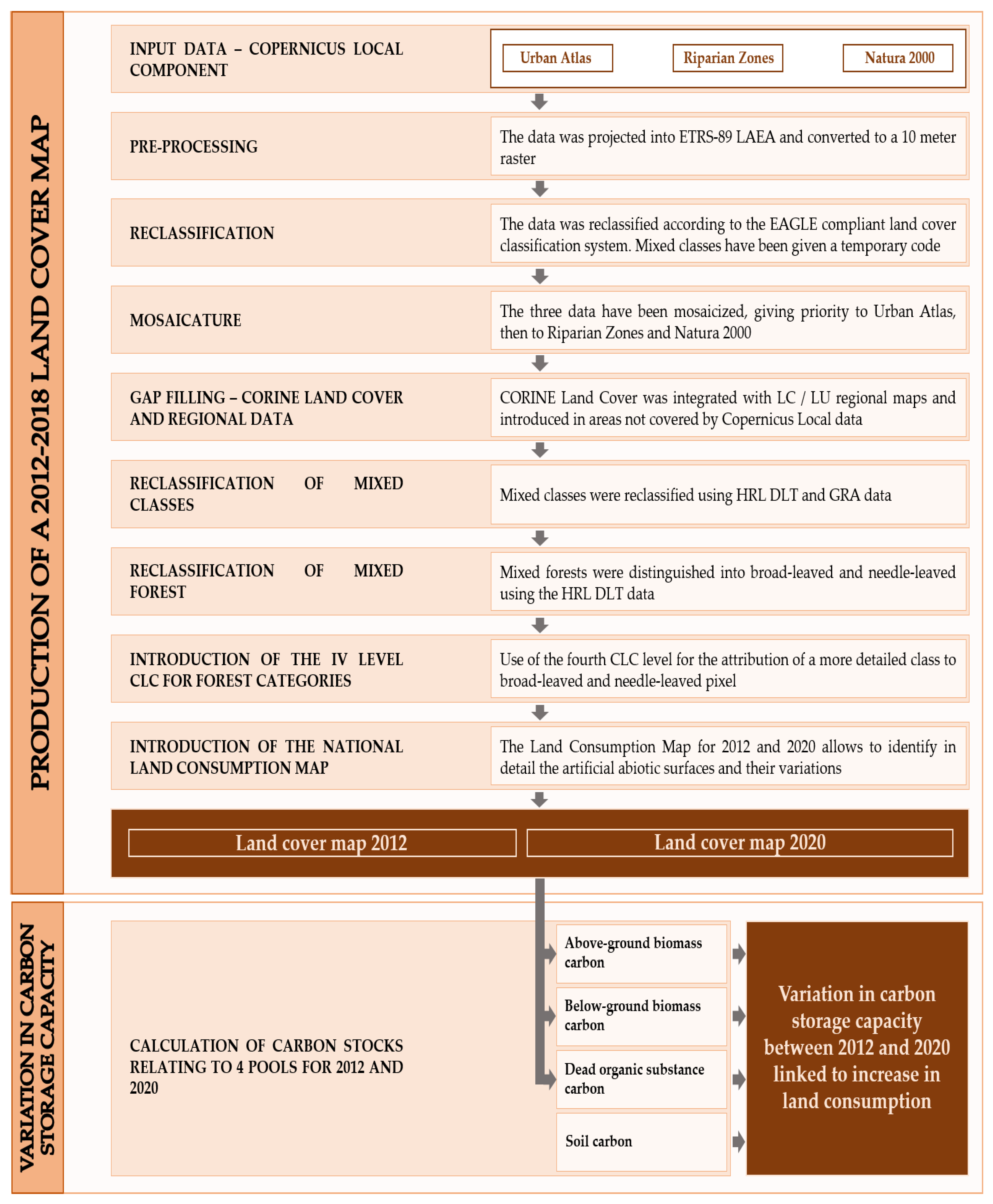
2.1. Overview
2.2. Study Area
2.3. Land Cover Classification System
- Abiotic non-vegetated: The class includes any unvegetated surfaces. At the second classification level, the class is subdivided between man-made artificial structures (artificial abiotic surfaces) and natural material surfaces (natural abiotic surfaces).
- 2.
- Biotic vegetated: The class includes any vegetated surfaces, with or without anthropogenic influence. At the second classification level, woody and herbaceous vegetation are distinguished.
- 3.
- Water surfaces: The class includes natural or artificial solid and liquid water. The second classification level distinguishes water bodies from permanent snow and ice. Water bodies includes liquid water regardless of shape, position, salinity and origin. Permanent snow and ice includes accumulations that persist throughout the year regardless of seasonal variations.
- 4.
- Wetlands: The class does not have a direct correspondence with the EAGLE LCC, as it is considered an LCH. The class was however included to maintain the information content offered by the input data. In detail, a definition was adopted aligned with the CORINE Land Cover, including in the class the inland wetlands (inland marshes and peat bogs) and coastal wetlands (salt marshes, salines, intertidal flats) while lagoons and estuaries are associated to water bodies.
2.4. Selection of Input Data
2.4.1. CLMS Data
2.4.2. National Data
2.5. Production of a National Land Cover Map Based on Copernius and National Data
2.5.1. Data Pre-Processing
2.5.2. Map Production
Reclassification of Copernicus UA, RZ, N2000 Data and Creation of the Basic Mosaic
Reclassification and Introduction of CLC Data and Regional Maps
Use of HRLs for the Classification of Uncertain Classes (Temporary Code 91–99)
Use of HRLs to Classify Broad-Leaved and Needle-Leaved in the Mixed Forest (Temporary Code 999)
Use of the Fourth CLC Level for the Attribution of a More Detailed Prevalent Class to Broad-Leaved and Needle-Leaved Pixel
Inclusion of LCM and Assignment of the Class to Temporary Codes 998
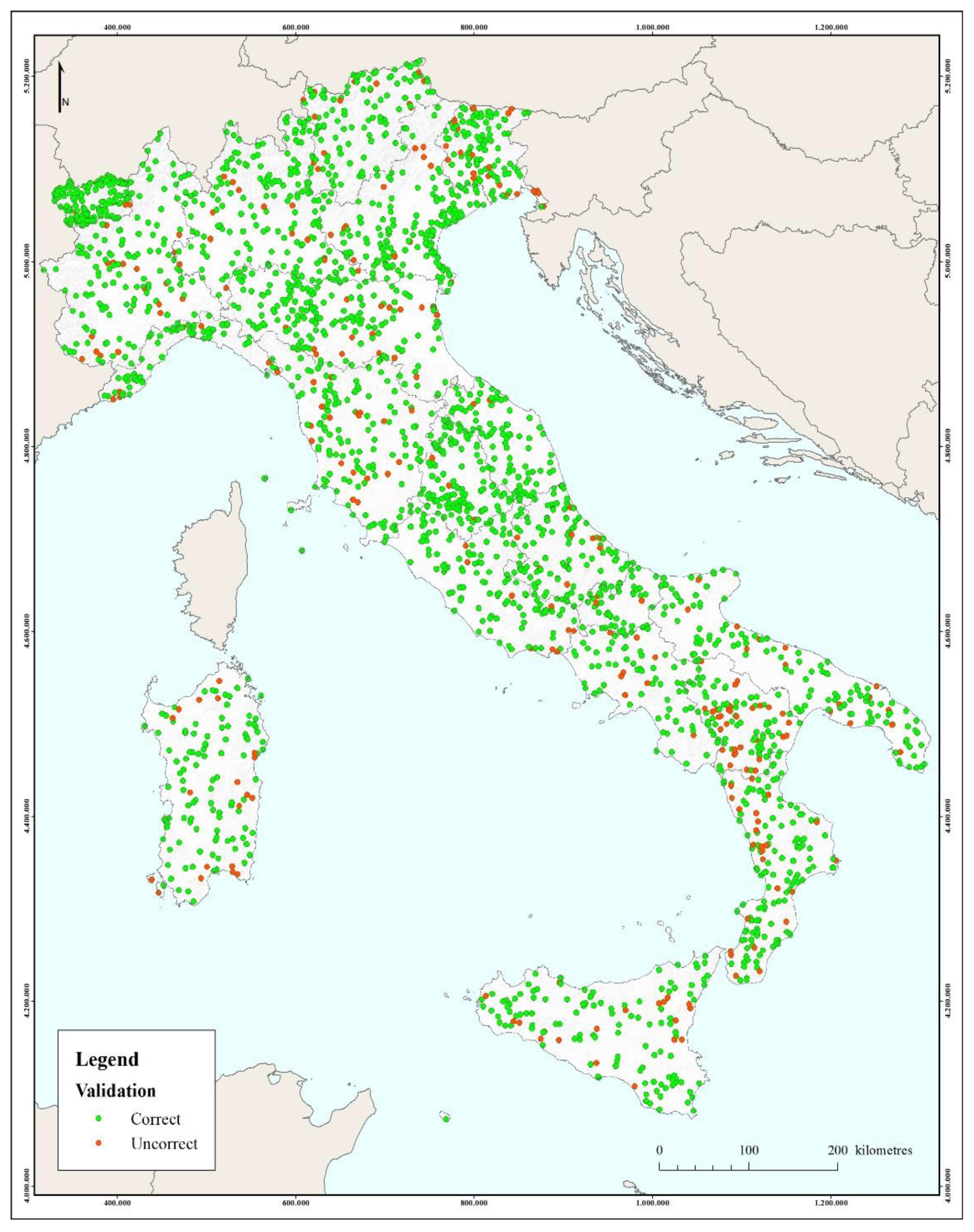
2.5.3. Accuracy Assessment
- Wi—is area proportion of each classes in the considered map
- Ui—user accuracy of class i. A conservative scenario was assumed, considering Ui = 0.6 for all classes.
- Si—standard deviation of stratum i, Si = √(Ui(1 − Ui)) [50]. Considering Ui = 0.6, it turns out Si = 0.49 for all classes.
- S(Ô)—is the target standard error for overall accuracy. It was assumed to be 0.01 as suggested by Olofsson [46], which corresponds to a confidence interval of 1%.
- A sample of size 2400 was obtained (Table 6).
2.5.4. Ecosystem Services—Carbon Storage Capacity Assessment
Above-Ground Biomass (AGB)
Below-Ground Biomass (BGB)
- GSV = growing stock volume
- BEF = biomass expansion factor
- WBD = wood basic density
The Carbon Contained in the Dead Organic Substance (DOS)
Soil Carbon
3. Results
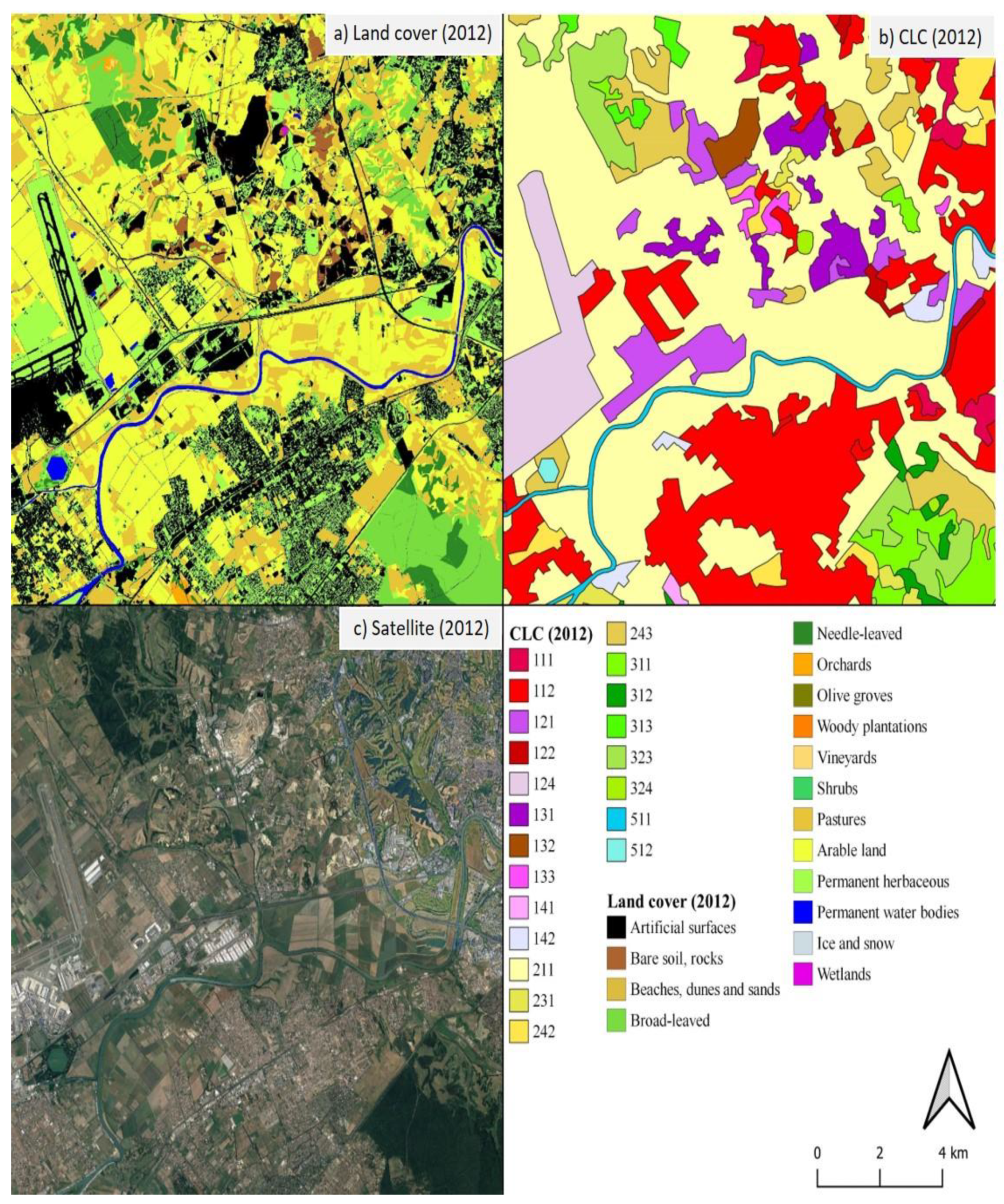
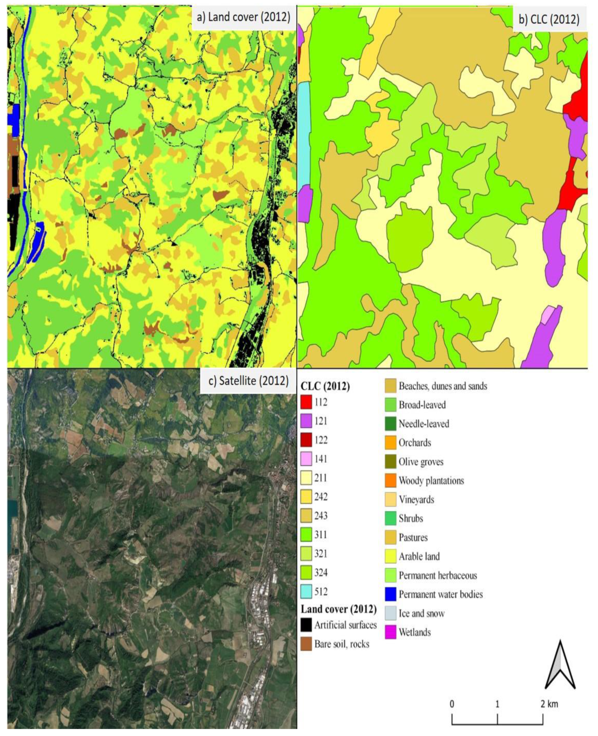
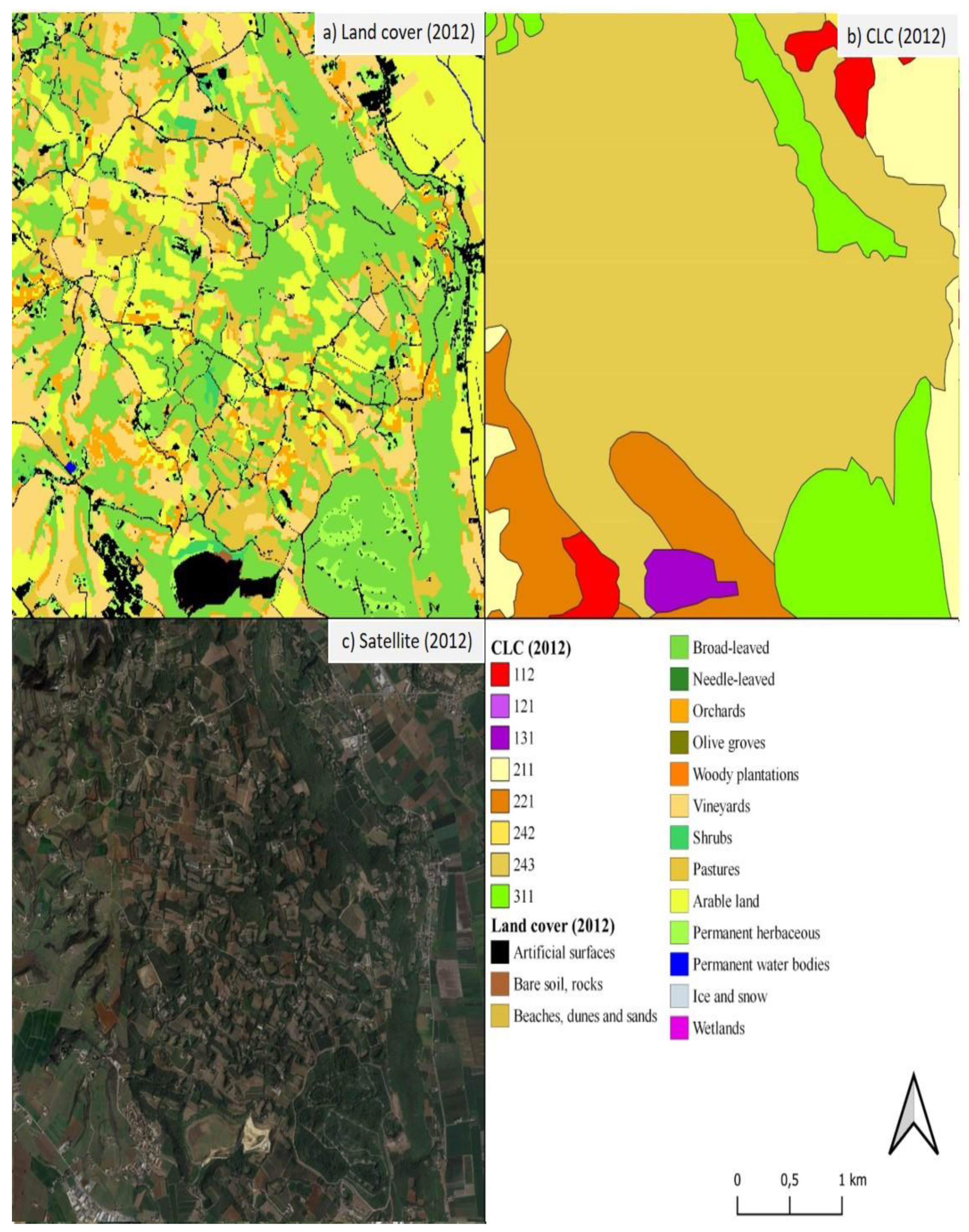
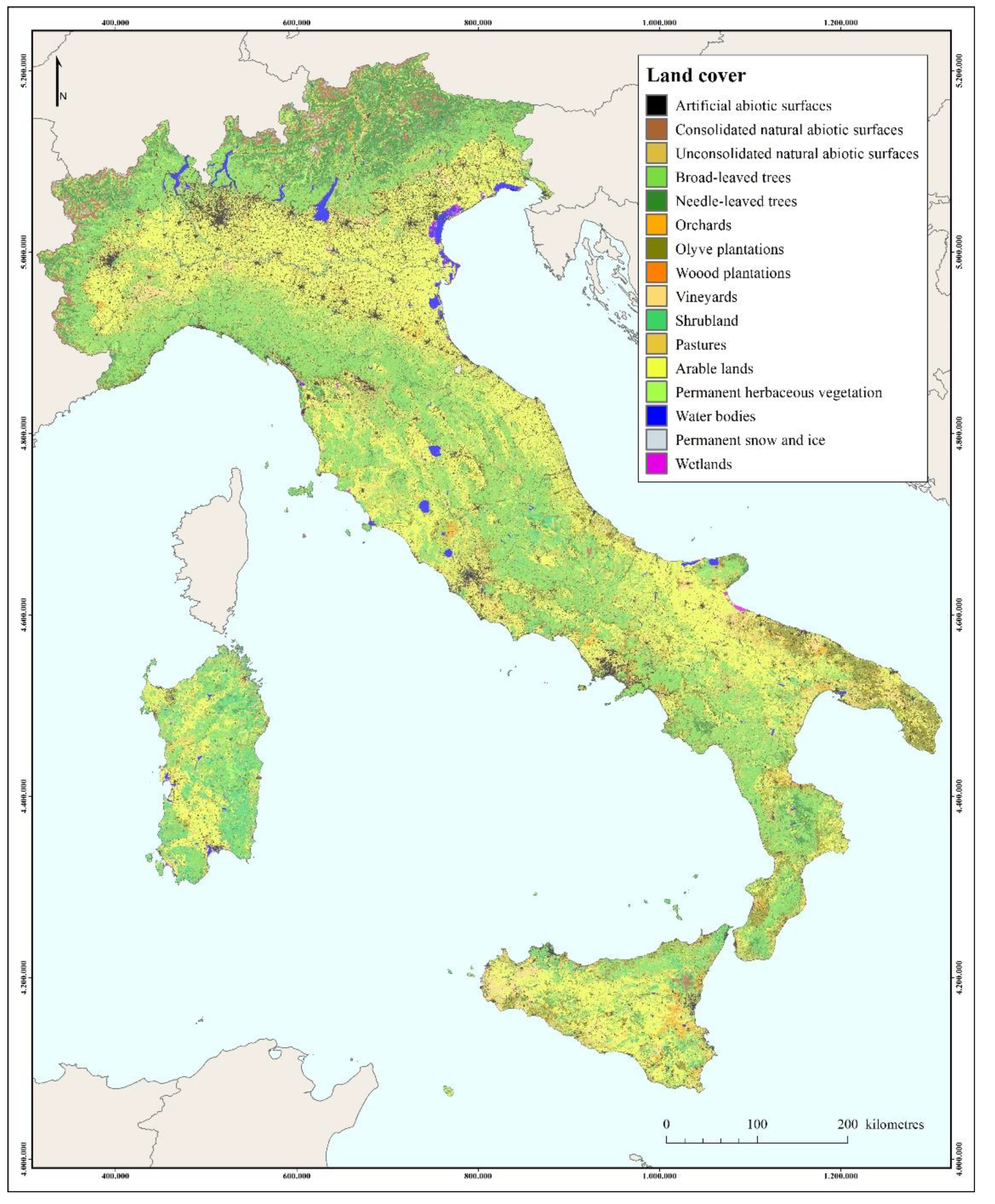
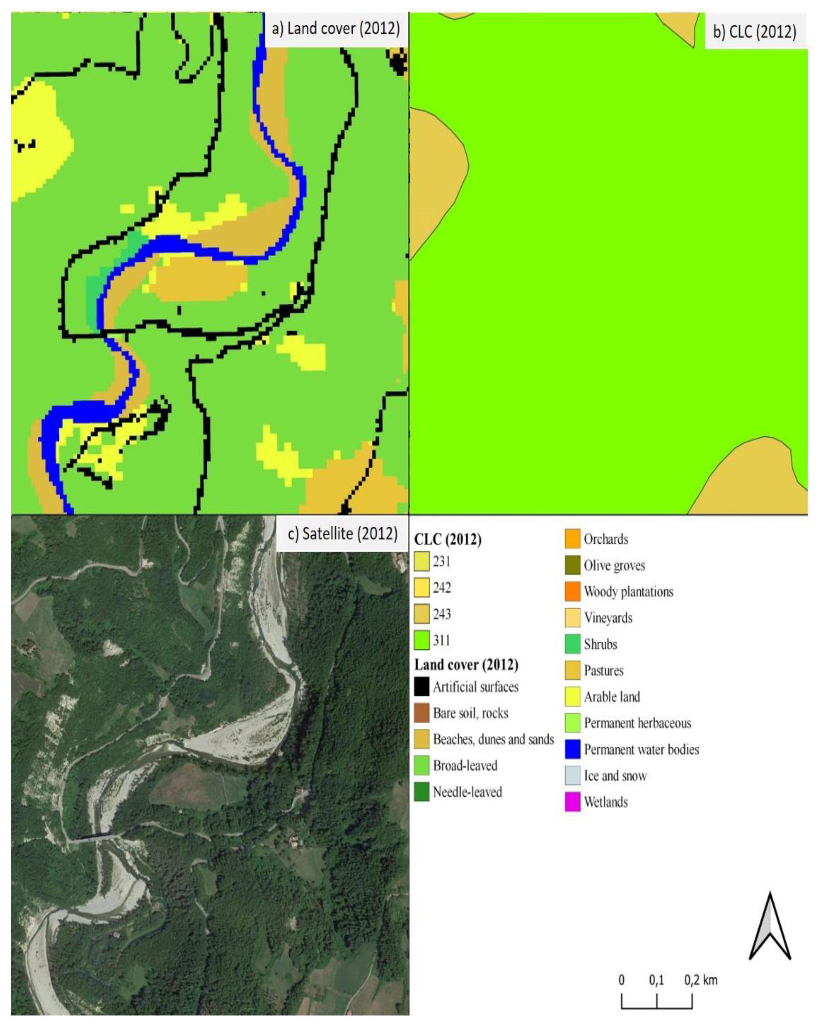
3.1. Land Cover Map and Accuracy Assessment
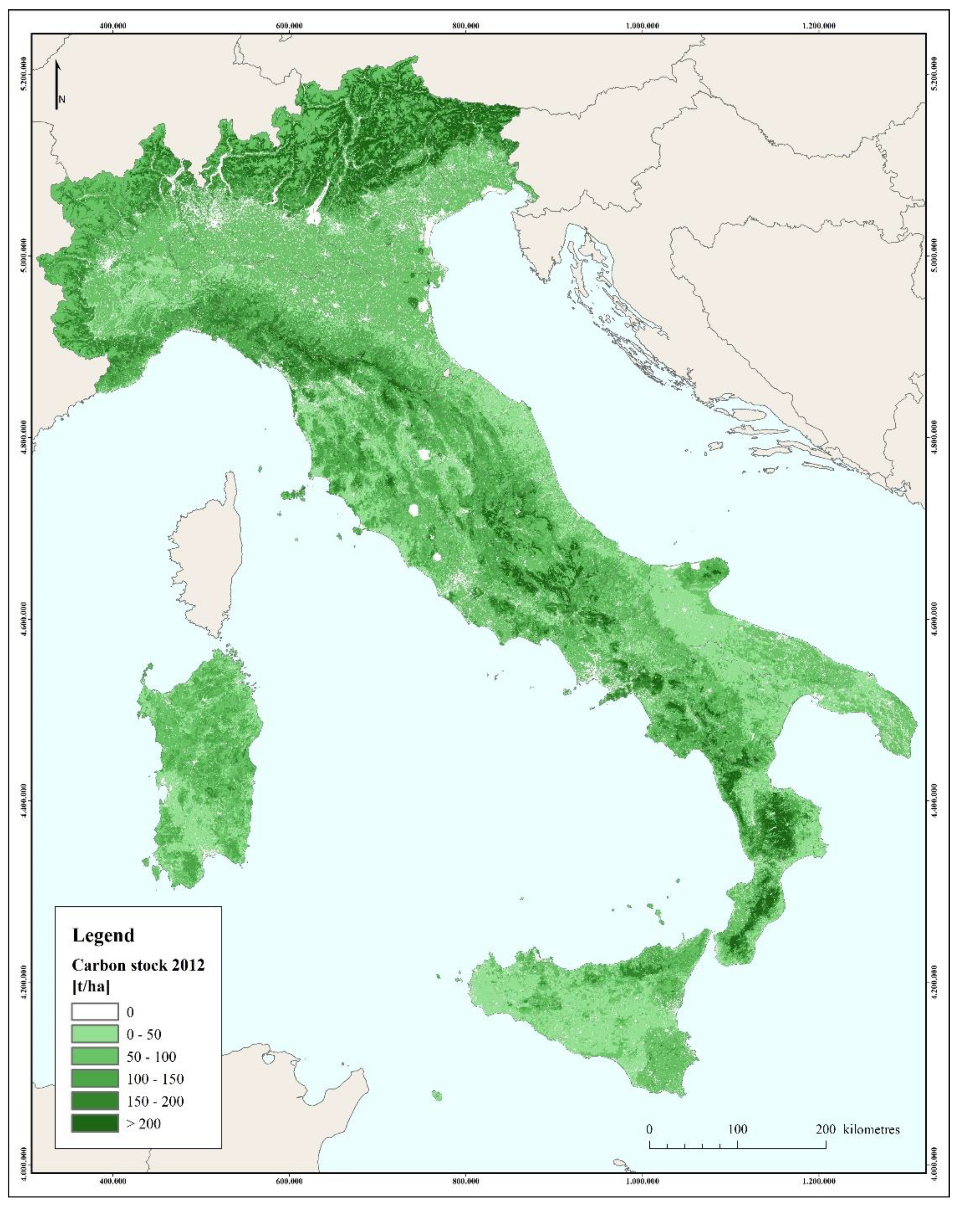
3.2. Estimation of the Carbon Storage Capacity
4. Discussion
5. Conclusions
Author Contributions
Funding
Institutional Review Board Statement
Informed Consent Statement
Data Availability Statement
Conflicts of Interest
Appendix A

| N2000 | Class Name | LC | N2000 | Class Name | LC |
|---|---|---|---|---|---|
| 1110 | Urban fabric (predominantly public and private units) | 998 | 4212 | Seminatural grassland without woody plants (C.C.D. ≤ 30%) | 93 |
| 1120 | Industrial, commercial and military units | 998 | 4220 | Alpine and subalpine natural grassland | 22200 |
| 1210 | Road networks and associated land | 998 | 5110 | Heathland and Moorland | 22200 |
| 1220 | Railways and associated land | 998 | 5120 | Other scrub land | 21220 |
| 1230 | Port areas and associated land | 998 | 5200 | Sclerophyllous vegetation | 21220 |
| 1240 | Airports and associated land | 998 | 6100 | Sparsely vegetated areas | 96 |
| 1310 | Mineral extraction, dump and construction sites | 998 | 6210 | Beaches and dunes | 12200 |
| 1320 | Land without current use | 998 | 6220 | River banks | 12200 |
| 1400 | Green urban, sports and leisure facilities | 998 | 6310 | Bare rocks and rock debris | 12100 |
| 2110 | Arable land | 22120 | 6320 | Burnt areas (except burnt forest) | 97 |
| 2120 | Greenhouses | 22120 | 6330 | Glaciers and perpetual snow | 32000 |
| 2210 | Vineyards, fruit trees and berry plantations | 99 | 7100 | Inland marshes | 40000 |
| 2220 | Olive groves | 21132 | 7210 | Exploited peat bog | 40000 |
| 2310 | Annual crops associated with permanent crops | 92 | 7220 | Unexploited peat bog | 40000 |
| 2320 | Complex cultivation patterns | 92 | 8110 | Coastal salt marshes | 40000 |
| 2330 | Land principally occupied by agriculture with significant areas of natural vegetation | 93 | 8120 | Salines | 40000 |
| 2340 | Agroforestry | 94 | 8130 | Intertidal flats | 40000 |
| 3110 | Natural and seminatural broad-leaved forest | 2111 | 8210 | Coastal lagoons | 31000 |
| 3120 | Highly artificial broad-leaved plantations | 2111 | 8220 | Estuaries | 31000 |
| 3210 | Natural and seminatural coniferous forest | 2112 | 9110 | Interconnected water courses | 31000 |
| 3220 | Highly artificial coniferous plantations | 2112 | 9120 | Highly modified water courses and canals | 31000 |
| 3310 | Natural and seminatural mixed forest | 999 | 9130 | Separated water bodies belonging to the river system | 31000 |
| 3320 | Highly artificial mixed plantations | 99 | 9210 | Natural water bodies | 31000 |
| 3410 | Transitional woodland and scrub | 95 | 9220 | Artificial standing water bodies | 31000 |
| 3420 | Lines of trees and scrub | 95 | 9230 | Intensively managed fish ponds | 31000 |
| 3500 | Damaged forest | 95 | 9240 | Standing water bodies of extractive industrial sites | 31000 |
| 4100 | Managed grassland | 22110 | 10000 | Sea and ocean | 31000 |
| 4211 | Seminatural grassland with woody plants (C.C.D. ≥ 30%) | 93 |
| UA | Class Name | LC | UA | Class Name | LC |
|---|---|---|---|---|---|
| 11100 | Continuous Urban Fabric (>80%) | 998 | 13400 | Land without current use | 998 |
| 11210 | Discontin. Dense Urban Fabric (50–80%) | 998 | 14100 | Green urban areas | 91 |
| 11220 | Discontin. Medium Density Urban Fabric (30–50%) | 998 | 14200 | Sports and leisure facilities | 998 |
| 11230 | Discontinuous Low Density Urban Fabric (10–30%) | 998 | 21000 | Arable land (annual crops) | 22120 |
| 11240 | Discontinuous Very Low Density Urban Fabric (<10%) | 998 | 22000 | Permanent crops (vineyards, fruit trees, olive groves) | 99 |
| 11300 | Isolated Structures | 998 | 23000 | Pastures | 22110 |
| 12100 | Industrial, commercial, public, military and private units | 998 | 24000 | Complex and mixed cultivation patterns | 92 |
| 12210 | Fast transit roads and associated land | 998 | 25000 | Orchards at the fringe of urban classes | 21131 |
| 12220 | Other roads and associated land | 998 | 31000 | Forests | 999 |
| 12230 | Railways and associated land | 998 | 32000 | Herbaceous vegetation associations (natural grassland, moors...) | 22200 |
| 12300 | Port areas | 998 | 33000 | Open spaces with little or no vegetations (beaches, dunes, bare rocks, glaciers) | 96 |
| 12400 | Airports | 998 | 40000 | Wetland | 40000 |
| 13100 | Mineral extraction and dump site | 998 | 50000 | Water bodies | 31000 |
| 13300 | Construction sites | 998 |
| RZ | Class Name | LC | RZ | Class Name | LC |
|---|---|---|---|---|---|
| 11110 | Continuous Urban Fabric (IMD ≥ 80%) | 998 | 41000 | Managed grassland | 22110 |
| 11120 | Dense Urban Fabric (IMD ≥ 30–80%) | 998 | 42100 | Seminatural grassland | 93 |
| 11130 | Low Density Fabric (IMD < 30%) | 998 | 42200 | Alpine and subalpine natural grassland | 22200 |
| 11200 | Industrial, commercial and military units | 998 | 51100 | Heathland and Moorland | 22200 |
| 12100 | Road networks and associated land | 998 | 51200 | Other scrub land | 21220 |
| 12200 | Railways and associated land | 998 | 52000 | Sclerophyllous vegetation | 21220 |
| 12300 | Port areas and associated land | 998 | 61000 | Sparsely vegetated areas | 96 |
| 12400 | Airports and associated land | 998 | 62100 | Beaches and dunes | 12200 |
| 13100 | Mineral extraction, dump and construction sites | 998 | 62200 | River banks | 12200 |
| 13200 | Land without current use | 998 | 63100 | Bare rocks and rock debris | 12100 |
| 14000 | Green urban, sports and leisure facilities | 998 | 63200 | Burnt areas (except burnt forest) | 97 |
| 21100 | Arable land | 22120 | 63300 | Glaciers and perpetual snow | 32000 |
| 21200 | Greenhouses | 22120 | 71000 | Inland marshes | 40000 |
| 22100 | Vineyards, fruit trees and berry plantations | 99 | 72100 | Exploited peat bog | 40000 |
| 22200 | Olive groves | 21132 | 72200 | Unexploited peat bog | 40000 |
| 23100 | Annual crops associated with permanent crops | 92 | 81100 | Coastal salt marshes | 40000 |
| 23200 | Complex cultivation patterns | 92 | 81200 | Salines | 40000 |
| 23300 | Land principally occupied by agriculture with significant areas of natural vegetation | 93 | 81300 | Intertidal flats | 40000 |
| 23400 | Agroforestry | 94 | 82100 | Coastal lagoons | 31000 |
| 31100 | Natural and seminatural broad-leaved forest | 2111 | 82200 | Estuaries | 31000 |
| 31200 | Highly artificial broad-leaved plantations | 2111 | 91100 | Interconnected water courses | 31000 |
| 32100 | Natural and seminatural coniferous forest | 2112 | 91200 | Highly modified water courses and canals | 31000 |
| 32200 | Highly artificial coniferous plantations | 2112 | 91300 | Separated water bodies belonging to the river system | 31000 |
| 33100 | Natural and seminatural mixed forest | 999 | 92100 | Natural water bodies | 31000 |
| 33200 | Highly artificial mixed plantations | 999 | 92200 | Artificial standing water bodies | 31000 |
| 34100 | Transitional woodland and scrub | 95 | 92300 | Intensively managed fish ponds | 31000 |
| 34200 | Lines of trees and scrub | 95 | 92400 | Standing water bodies of extractive industrial sites | 31000 |
| 35000 | Damaged forest | 95 | 10000 | Sea and ocean | 31000 |
| CLC | Class Name | LC | CLC | Class Name | LC |
|---|---|---|---|---|---|
| 111 | Continuous urban fabric | 998 | 31113117 | Broad-leaved forest | 2111 |
| 112 | Discontinuous urban fabric | 998 | 31213125 | Needle-leaved forest | 2112 |
| 121 | Industrial or commercial units | 998 | 31313132 | Mixed forest | 999 |
| 1211 | Photovoltaic fiends | 998 | 3211 | Continuous natural grasslands | 22200 |
| 122 | Road and rail networks and associated land | 998 | 3212 | Discontinuous natural grasslands | 22200 |
| 123 | Port areas | 998 | 322 | Moors and heathland | 21220 |
| 124 | Airports | 998 | 3231 | High Mediterranean scrub | 21220 |
| 131 | Mineral extraction sites | 998 | 3232 | Low Mediterranean scrub and the garrigue | 21220 |
| 132 | Dump sites | 998 | 324 | Transitional woodland shrub | 95 |
| 133 | Construction sites | 998 | 3241 | Forest harvesting | 95 |
| 141 | Green urban areas | 91 | 331 | Beaches, dunes, sands | 12200 |
| 142 | Sport and leisure facilities | 998 | 332 | Bare rocks | 12100 |
| 2111 | Intensive nonirrigated arable land | 22120 | 333 | Sparsely vegetated areas | 96 |
| 2112 | Extensive nonirrigated arable land | 22120 | 334 | Burnt areas | 97 |
| 212 | Permanently irrigated land | 22120 | 335 | Glaciers and perpetual snow | 32000 |
| 213 | Rice fields | 22120 | 411 | Inland marshes | 40000 |
| 221 | Vineyards | 21210 | 412 | Peat bogs | 40000 |
| 222 | Fruit trees and berry plantations | 21131 | 421 | Salt marshes | 40000 |
| 223 | Olive groves | 21132 | 422 | Salines | 40000 |
| 224 | Woody plantation | 21133 | 423 | Intertidal flats | 40000 |
| 2241 | New woody plantation | 21133 | 511 | Water courses | 31000 |
| 231 | Pastures | 22110 | 512 | Water bodies | 31000 |
| 241 | Annual crops associated with permanent crops | 92 | 521 | Coastal lagoons | 31000 |
| 242 | Complex cultivation patterns | 92 | 522 | Estuaries | 31000 |
| 243 | Land principally occupied by agriculture, with significant areas of natural vegetation | 93 | 523 | Sea and ocean | 31000 |
| 244 | Agroforestry | 94 |
References
- Munafò, M. Consumo di Suolo, Dinamiche Territoriali e Servizi Ecosistemici—Edizione 2018; ISPRA: Rome, Italy, 2018. [Google Scholar]
- Verburg, P.H.; Erb, K.-H.; Mertz, O.; Espindola, G. Land System Science: Between global challenges and local realities. Curr. Opin. Environ. Sustain. 2013, 5, 433–437. [Google Scholar] [CrossRef] [PubMed] [Green Version]
- Pedroli, G.B.M.; Meiner, A. Landscapes in Transition: An Account of 25 Years of Land Cover Change in Europe; European Environment Agency: København, Denmark, 2017. [Google Scholar]
- EEA. Land Systems at European Level—Analytical Assessment Framework. 2018. Briefing no. 10/2018. pp. 1–9. Available online: https://www.eea.europa.eu/themes/landuse/land-systems (accessed on 28 November 2021).
- Anderson, J.R. Land use and land cover changes. A framework for monitoring. J. Res. Geol. Surv. 1977, 5, 143–153. [Google Scholar]
- Liu, R.; Dong, X.; Wang, X.; Zhang, P.; Liu, M.; Zhang, Y. Study on the relationship among the urbanization process, ecosystem services and human well-being in an arid region in the context of carbon flow: Taking the Manas river basin as an example. Ecol. Indic. 2021, 132, 108248. [Google Scholar] [CrossRef]
- Costanza, R.; D’Arge, R.; de Groot, R.; Farberll, S.; Grassot, M.; Hannon, B.; Limburg, K.; Naeem, S.; O’Neilltt, R.V.; Paruelo, J.; et al. The value of the world’s ecosystem services and natural capital. Nature 1997, 387115, 253–260. [Google Scholar] [CrossRef]
- Gómez-Baggethun, E.; De Groot, R.; Lomas, P.L.; Montes, C. The history of ecosystem services in economic theory and practice: From early notions to markets and payment schemes. Ecol. Econ. 2010, 69, 1209–1218. [Google Scholar] [CrossRef]
- Danley, B.; Widmark, C. Evaluating conceptual definitions of ecosystem services and their implications. Ecol. Econ. 2016, 126, 132–138. [Google Scholar] [CrossRef]
- Teague, A.; Russell, M.; Harvey, J.; Dantin, D.; Nestlerode, J.; Alvarez, F. A spatially-explicit technique for evaluation of alternative scenarios in the context of ecosystem goods and services. Ecosyst. Serv. 2016, 20, 15–29. [Google Scholar] [CrossRef]
- Corvalan, C.; Hales, S.; McMichael, A.; Butler, C.; Campbell-Lendrum, D.; Confalonieri, U.; Leitner, K.; Lewis, N.; Patz, J.; Polson, K.; et al. A Report of the Millennium Ecosystem Assessment. In Ecosystems and Human Well-Being; Island Press: Washington, DC, USA, 2005; Volume 5. [Google Scholar]
- Xepapadeas, A. The Economics of Ecosystems and Biodiversity: Ecological and Economic Foundations; Kumar, P., Ed.; Earthscan: London, UK; Washington, DC, USA, 2011; Volume 16, pp. 239–242. ISBN 978-1-84971-212-5 (HB). [Google Scholar]
- La Notte, A.; D’Amato, D.; Mäkinen, H.; Paracchini, M.L.; Liquete, C.; Egoh, B.; Geneletti, D.; Crossman, N.D. Ecosystem services classification: A systems ecology perspective of the cascade framework. Ecol. Indic. 2017, 74, 392–402. [Google Scholar] [CrossRef]
- Potschin, M.; Haines-Young, R. Defining and measuring ecosystem services. In Routledge Handbook of Ecosystem Services; Potschin, M., Haines-Young, R., Fish, R., Turner, R.K., Eds.; Routledge: London, UK; New York, NY, USA, 2016; pp. 25–44. [Google Scholar]
- Costanza, R.; de Groot, R.; Sutton, P.; van der Ploeg, S.; Anderson, S.J.; Kubiszewski, I.; Farber, S.; Turner, R.K. Changes in the global value of ecosystem services. Glob. Environ. Chang. 2014, 26, 152–158. [Google Scholar] [CrossRef]
- Zulian, G.; Maes, J.; Paracchini, M.L. Linking land cover data and crop yields for mapping and assessment of pollination services in Europe. Land 2013, 2, 472–492. [Google Scholar] [CrossRef] [Green Version]
- Groff, S.C.; Loftin, C.S.; Drummond, F.; Bushmann, S.; McGill, B. Parameterization of the InVEST crop pollination model to spatially predict abundance of wild blueberry (Vaccinium angustifolium Aiton) native bee pollinators in Maine, USA. Environ. Model. Softw. 2016, 79, 1–9. [Google Scholar] [CrossRef] [Green Version]
- Leonhardt, S.D.; Gallai, N.; Garibaldi, L.A.; Kuhlmann, M.; Klein, A.-M. Economic gain, stability of pollination and bee diversity decrease from southern to northern Europe. Basic Appl. Ecol. 2013, 14, 461–471. [Google Scholar] [CrossRef]
- Lautenbach, S.; Seppelt, R.; Liebscher, J.; Dormann, C.F. Spatial and temporal trends of global pollination benefit. PLoS ONE 2012, 7, e35954. [Google Scholar] [CrossRef] [PubMed] [Green Version]
- Hanley, N.; Breeze, T.D.; Ellis, C.; Goulson, D. Measuring the economic value of pollination services: Principles, evidence and knowledge gaps. Ecosyst. Serv. 2015, 14, 124–132. [Google Scholar] [CrossRef] [Green Version]
- UK National Ecosystem Assessment. The UK National Ecosystem Assessment: Synthesis of the Key Findings; UNEP-WCMC: Cambridge, UK, 2011. [Google Scholar]
- Rabe, S.-E.; Koellner, T.; Marzelli, S.; Schumacher, P.; Grêt-Regamey, A. National ecosystem services mapping at multiple scales. The German exemplar. Ecol. Indic. 2016, 70, 357–372. [Google Scholar] [CrossRef]
- Santos-Martín, F.; García Llorente, M.; Quintas-Soriano, C.; Zorrilla-Miras, P.; Martín-Lopez, B.; Loureiro, M.; Benayas, J.; Montes, M. Spanish National Ecosystem Assessment: Socio-economic valuation of ecosystem services in Spain. Synthesis of the key findings; Biodiversity Foundation of the Spanish Ministry of Agriculture, Food and Environment: Madrid, Spain, 2016.
- Xie, G.; Zhang, C.; Zhen, L.; Zhang, L. Dynamic changes in the value of China’s ecosystem services. Ecosyst. Serv. 2017, 26, 146–154. [Google Scholar] [CrossRef]
- Turpie, J.K.; Forsythe, K.J.; Knowles, A.; Blignaut, J.; Letley, G. Mapping and valuation of South Africa’s ecosystem services: A local perspective. Ecosyst. Serv. 2017, 27, 179–192. [Google Scholar] [CrossRef]
- Choi, H.-A.; Song, C.; Lee, W.-K.; Jeon, S.; Gu, J.H. Integrated approaches for national ecosystem assessment in South Korea. KSCE J. Civ. Eng. 2018, 22, 1634–1641. [Google Scholar] [CrossRef]
- Daily, G.C.; Matson, P.A.; Vitousek, P.M. Ecosystem services supplied by soil. In Nature’s Services: Societal Dependence on Natural Ecosystems; Daily, G.C., Ed.; Island Press: Washington, DC, USA, 1997; pp. 113–132. [Google Scholar]
- Wall, D.H.; Bardgett, R.D.; Covich, A.P.; Snelgrove, P.V.R. The Need for Understanding How Biodiversity and Ecosystem Functioning Affect Ecosystem Services in Soils and Sediments; Island Press: Washington, DC, USA, 2004. [Google Scholar]
- Dominati, E.; Patterson, M.; Mackay, A. A framework for classifying and quantifying the natural capital and ecosystem services of soils. Ecol. Econ. 2010, 69, 1858–1868. [Google Scholar] [CrossRef]
- Fryer, J.; Williams, I.D. Regional carbon stock assessment and the potential effects of land cover change. Sci. Total Environ. 2021, 775, 145815. [Google Scholar] [CrossRef] [PubMed]
- Mathew, I.; Shimelis, H.; Mutema, M.; Minasny, B.; Chaplot, V. Crops for increasing soil organic carbon stocks–A global meta analysis. Geoderma 2020, 367, 114230. [Google Scholar] [CrossRef]
- Clerici, N.; Cote-Navarro, F.; Escobedo, F.J.; Rubiano, K.; Villegas, J.C. Spatio-temporal and cumulative effects of land use-land cover and climate change on two ecosystem services in the Colombian Andes. Sci. Total Environ. 2019, 685, 1181–1192. [Google Scholar] [CrossRef]
- Savaresi, A.; Perugini, L.; Chiriacò, M.V. Making sense of the LULUCF Regulation: Much ado about nothing? Rev. Eur. Comp. Int. Environ. Law 2020, 29, 212–220. [Google Scholar] [CrossRef]
- Sallustio, L.; Quatrini, V.; Geneletti, D.; Corona, P.; Marchetti, M. Assessing land take by urban development and its impact on carbon storage: Findings from two case studies in Italy. Environ. Impact Assess. Rev. 2015, 54, 80–90. [Google Scholar] [CrossRef] [Green Version]
- Vashum, K.T.; Jayakumar, S. Methods to estimate above-ground biomass and carbon stock in natural forests-a review. J. Ecosyst. Ecography 2012, 2, 1–7. [Google Scholar] [CrossRef]
- Sallustio, L.; Munafò, M.; Riitano, N.; Lasserre, B.; Fattorini, L.; Marchetti, M. Integration of land use and land cover inventories for landscape management and planning in Italy. Environ. Monit. Assess. 2016, 188, 48. [Google Scholar] [CrossRef]
- Maes, J.; Teller, A.; Erhard, M.; Liquete, C.; Braat, L.; Berry, P.; Egoh, B.; Puydarrieus, P.; Fiorina, C.; Santos, F.; et al. An Analytical Framework for Ecosystem Assessments under Action 5 of the EU Biodiversity Strategy to 2020; Publications Office of the European Union: Luxembourg, 2013; ISBN 9789279293696. [Google Scholar]
- Cabral, P.; Feger, C.; Levrel, H.; Chambolle, M.; Basque, D. Assessing the impact of land-cover changes on ecosystem services: A first step toward integrative planning in Bordeaux, France. Ecosyst. Serv. 2016, 22, 318–327. [Google Scholar] [CrossRef] [Green Version]
- Arnold, S.; Kosztra, B.; Banko, G.; Smith, G.; Hazeu, G.; Bock, M. The EAGLE concept—A vision of a future European Land Monitoring Framework. In Proceedings of the 33th EARSeL Symposium towards Horizon 2020, Matera, Italy, 3–6 June 2013; pp. 551–568. [Google Scholar]
- Kleeschulte, S. Technical Specifications for Implementation of a New Land-Monitoring Concept Based on EAGLE. D3: Draft Design Concept and CLC-Backbone, CLC-Core Technical Specifications, Including Requirements Review, 3rd ed.; European Environment Agency: Copenhagen, Denmark, 2019; p. 78. [Google Scholar]
- De Fioravante, P.; Luti, T.; Cavalli, A.; Giuliani, C.; Dichicco, P.; Marchetti, M.; Chirici, G.; Congedo, L.; Munafò, M. Multispectral Sentinel-2 and SAR Sentinel-1 Integration for Automatic Land Cover Classification. Land 2021, 10, 611. [Google Scholar] [CrossRef]
- Munafò, M. Consumo di Suolo, Dinamiche Territoriali e Servizi Ecosistemici. Edizione 2020; ISPRA: Rome, Italy, 2020. [Google Scholar]
- Munafò, M. Consumo di Suolo, Dinamiche Territoriali e Servizi Ecosistemici Edizione 2021 Rapporto ISPRA SNPA; ISPRA: Rome, Italy, 2021; ISBN 9788844810597. [Google Scholar]
- Luti, T.; De Fioravante, P.; Marinosci, I.; Strollo, A.; Riitano, N.; Falanga, V.; Mariani, L.; Congedo, L.; Munafò, M. Land Consumption Monitoring with SAR Data and Multispectral Indices. Remote Sens. 2021, 13, 1586. [Google Scholar] [CrossRef]
- Strollo, A.; Smiraglia, D.; Bruno, R.; Assennato, F.; Congedo, L.; De Fioravante, P.; Giuliani, C.; Marinosci, I.; Riitano, N.; Munafò, M. Land consumption in Italy. J. Maps 2020, 16, 113–123. [Google Scholar] [CrossRef]
- Olofsson, P.; Foody, G.M.; Herold, M.; Stehman, S.V.; Woodcock, C.E.; Wulder, M.A. Good practices for estimating area and assessing accuracy of land change. Remote Sens. Environ. 2014, 148, 42–57. [Google Scholar] [CrossRef]
- FAO Map Accuracy Assessment and Area Estimation: A Practical Guide. National Forest Monitoring and Assessment Working Paper. 2016. 46/E. p. 69. Available online: https://www.fao.org/publications/card/fr/c/e5ea45b8-3fd7-4692-ba29-fae7b140d07e/ (accessed on 28 November 2021).
- Stehman, S.V.; Czaplewski, R.L. Design and Analysis for Thematic Map Accuracy Assessment—An application of satellite imagery. Remote Sens. Environ. 1998, 64, 331–344. [Google Scholar] [CrossRef]
- Stehman, S.V.; Foody, G.M. Key issues in rigorous accuracy assessment of land cover products. Remote Sens. Environ. 2019, 231, 111199. [Google Scholar] [CrossRef]
- Cochran, W.G.; William, G. Sampling Techniques; John Wiley& Sons: New York, NY, USA, 1977. [Google Scholar]
- Lupia, F. MARSALa-A Model-Based Irrigation Water Consumption Estimation at Farm Level; INEA: Brussels, Belgium, 2013. [Google Scholar]
- Vitullo, M.; De Lauretis, R.; Federici, S. La Contabilità del Carbonio Contenuto Nelle Foreste Italiane; Agenzia per la Protezione dell’ambiente e per i Servizi Tecnici: Rome, Italy, 2007. [Google Scholar]
- Di Cosmo, L.; Gasparini, P.; Tabacchi, G. A national-scale, stand-level model to predict total above-ground tree biomass from growing stock volume. For. Ecol. Manag. 2016, 361, 269–276. [Google Scholar] [CrossRef]
- Romano, D.; Arcarese, C.; Bernetti, A.; Caputo, A.; Contaldi, M.; De Lauretis, R.; Di Cristofaro, E.; Gagna, A.; Gonella, B.; Taurino, E.; et al. Italian Greenhouse Gas Inventory 1990–2015. National Inventory Report 2017. 2017. Available online: https://www.isprambiente.gov.it/en/publications/reports/italian-greenhouse-gas-inventory-1990-2015.-national-inventory-report-2017 (accessed on 28 November 2021).
- Li, S.; Liu, Y.; Yang, H.; Yu, X.; Zhang, Y.; Wang, C. Integrating ecosystem services modeling into effectiveness assessment of national protected areas in a typical arid region in China. J. Environ. Manag. 2021, 297, 113408. [Google Scholar] [CrossRef]
- Penman, J.; Gytarsky, M.; Hiraishi, T.; Krug, T.; Kruger, D.; Pipatti, R.; Buendia, L.; Miwa, K.; Ngara, T.; Tanabe, K. Good practice guidance for land use, land-use change and forestry. Good Pract. Guid. L. Use Land-Use Chang. For. 2003. Available online: https://www.ipcc.ch/publication/good-practice-guidance-for-land-use-land-use-change-and-forestry/ (accessed on 28 November 2021).
- Marchetti, M.; Sallustio, L.; Ottaviano, M.; Barbati, A.; Corona, P.; Tognetti, R.; Zavattero, L.; Capotorti, G. Carbon sequestration by forests in the National Parks of Italy. Plant Biosyst. Int. J. Deal. Asp. Plant Biol. 2012, 146, 1001–1011. [Google Scholar] [CrossRef]
- Canaveira, P.; Manso, S.; Pellis, G.; Perugini, L.; De Angelis, P.; Neves, R.; Papale, D.; Paulino, J.; Pereira, T.; Pina, A. Biomass Data on Cropland and Grassland in the Mediterranean Region. Final Report for Action A4 of Project MediNet. 2018. Available online: http://www.lifemedinet.com/ (accessed on 28 November 2021).
- Burke, T.; Whyatt, J.D.; Rowland, C.; Blackburn, G.A.; Abbatt, J. The influence of land cover data on farm-scale valuations of natural capital. Ecosyst. Serv. 2020, 42, 101065. [Google Scholar] [CrossRef]
- Tomlinson, S.J.; Dragosits, U.; Levy, P.E.; Thomson, A.M.; Moxley, J. Quantifying gross vs. net agricultural land use change in Great Britain using the Integrated Administration and Control System. Sci. Total Environ. 2018, 628, 1234–1248. [Google Scholar] [PubMed]
- Morel, J.L.; Chenu, C.; Lorenz, K. Ecosystem services provided by soils of urban, industrial, traffic, mining, and military areas (SUITMAs). J. Soils Sediments 2015, 15, 1659–1666. [Google Scholar] [CrossRef]
- Sambucini, V.; Marinosci, I.; Bonora, N.; Chirci, G. La Realizzazione in Italia del Progetto CORINE Land Cover 2006; ISPRA: Rome, Italy, 2010; ISBN 9788844804770. [Google Scholar]
- Tomaselli, V.; Dimopoulos, P.; Marangi, C.; Kallimanis, A.S.; Adamo, M.; Tarantino, C.; Panitsa, M.; Terzi, M.; Veronico, G.; Lovergine, F. Translating land cover/land use classifications to habitat taxonomies for landscape monitoring: A Mediterranean assessment. Landsc. Ecol. 2013, 28, 905–930. [Google Scholar] [CrossRef] [Green Version]
- Spadoni, G.L.; Cavalli, A.; Congedo, L.; Munafò, M. Analysis of Normalized Difference Vegetation Index (NDVI) multi-temporal series for the production of forest cartography. Remote Sens. Appl. Soc. Environ. 2020, 20, 100419. [Google Scholar] [CrossRef]


| Land Cover | |||||||||
|---|---|---|---|---|---|---|---|---|---|
| I Level | II Level | III Level | IV Level | V Level | |||||
| 1 | Abiotic Non-vegetated surfaces | 11 | Artificial abiotic | ||||||
| 12 | Natural abiotic | 121 | Consolidated (bare rocks, cliffs) | ||||||
| 122 | Unconsolidated (beaches, dunes, sands) | ||||||||
| 2 | Biotic vegetated surfaces | 21 | Woody vegetation | 211 | Trees | 2111 | Broad-leaved | ||
| 2112 | Needle-leaved | ||||||||
| 2113 | Permanent crops | 21131 | Orchards | ||||||
| 21132 | Olive groves | ||||||||
| 21133 | Wood plantations | ||||||||
| 212 | Shrubs | 2121 | Vineyards | ||||||
| 2122 | Shrubland | ||||||||
| 22 | Herbaceous vegetation | 221 | Periodically | 2211 | Pastures | ||||
| 2212 | Arable land | ||||||||
| 222 | Permanent | ||||||||
| 3 | Water surfaces | 31 | Water bodies | ||||||
| 32 | Permanent snow and ice | ||||||||
| 4 | Wetlands | ||||||||
| Urban Atlas | Riparian Zones | Natura 2000 | |
|---|---|---|---|
| Data type | Vector | Vector | Vector |
| Classes | 27 | 56 | 55 |
| MMU | 0.25 ha (class 1) 1 ha (class 2–5) | 0.5 ha | 0.5 ha |
| High Resolution Layers | CORINE Land Cover | |
|---|---|---|
| Data type | Raster | Vector |
| Classes | 4 | 44 |
| MMU | Pixel 10 × 10 m | 25 ha (status) 5 ha (changes) |
| Temporary Codes | UA | RZ | N2000 | CLC | |
|---|---|---|---|---|---|
| 91 | Green urban areas | 14100 | 141 | ||
| 92 | Annual crops associated with permanent crops | 23100 | 2310 | 241 | |
| Complex cultivation patterns | 24000 | 23200 | 2320 | 242 | |
| 93 | Land principally occupied by agriculture with significant areas of natural vegetation | 23300 | 2330 | 243 | |
| 94 | Agroforestry | 23400 | 2340 | 244 | |
| 95 | Transitional woodland and scrub | 34100 | 3410 | 324 | |
| Damaged forest | 3500 | ||||
| 96 | Sparsely vegetated areas | 33000 | 61000 | 6100 | 333 |
| 97 | Burnt areas | 63200 | 6320 | 334 | |
| 99 | Permanent crops (vineyards, fruit trees, olive groves) | 22000 | 22100 | 2210 | |
| 998 | Urban areas and artificial surfaces | 11100–13400, 14200 | 11110–14000 | 1110–1400 | 111–133, 142 |
| 999 | Mixed forest | 31000 | 33100 | 3131–3132 | |
| Temporary Code | Area Covered by DLT | Area Covered by GRA | No GRA and No DLT Area | |||
|---|---|---|---|---|---|---|
| 91 | 21131 | Orchards | 2211 | Pastures | 2121 | Vineyards |
| 92 | 2212 | Arable land | ||||
| 93 | 2111 or 2112 | Broad-leaved or Needle-leaved | 2211 | Pastures | 2212 | Arable land |
| 94 | 2212 | Arable land | ||||
| 95 | 2122 | Shrubland | ||||
| 96 | 222 | Permanent | ||||
| 97 | 222 | Permanent | 121 | Natural abiotic surfaces | ||
| 99 | 21131 | Orchards | 2121 | Vineyards | ||
| Land Cover Class | Area (ha) | Wi | Wi*Si |
|---|---|---|---|
| Artificial abiotic surfaces | 2,102,288 | 0.070 | 0.034 |
| Consolidated (bare rocks, cliffs) | 802,539 | 0.027 | 0.013 |
| Unconsolidated (beaches, dunes, sands) | 59,325 | 0.002 | 0.001 |
| Broad-leaved | 7,805,217 | 0.259 | 0.127 |
| Needle-leaved | 2,167,261 | 0.072 | 0.035 |
| Orchards | 619,759 | 0.021 | 0.010 |
| Olive plantations | 1,088,099 | 0.036 | 0.018 |
| Wood plantations | 46,356 | 0.002 | 0.001 |
| Vineyards | 689,746 | 0.023 | 0.011 |
| Shrubland | 1,375,125 | 0.046 | 0.022 |
| Pastures | 1,372,790 | 0.046 | 0.022 |
| Arable land | 9,183,519 | 0.305 | 0.149 |
| Permanent herbaceous | 2,337,826 | 0.078 | 0.038 |
| Water bodies | 402,830 | 0.013 | 0.007 |
| Permanent snow and ice | 37,000 | 0.001 | 0.001 |
| Wetlands | 50,295 | 0.002 | 0.001 |
| Total | 30,139,975 | 1 | |
| Total number of samples | 2400 | ||
| Classes | Allocation | ||
|---|---|---|---|
| Equal | Proportional | Final | |
| Artificial abiotic surfaces | 150 | 167 | 159 |
| Consolidated(bare rocks, cliffs) | 150 | 64 | 107 |
| Unconsolidated (beaches, dunes, sands) | 150 | 5 | 100 |
| Broad-leaved | 150 | 622 | 386 |
| Needle-leaved | 150 | 173 | 162 |
| Orchards | 150 | 49 | 100 |
| Olive plantations | 150 | 87 | 119 |
| Wood plantations | 150 | 4 | 77 |
| Vineyards | 150 | 55 | 103 |
| Shrubland | 150 | 109 | 130 |
| Pastures | 150 | 109 | 130 |
| Arable land | 150 | 731 | 441 |
| Permanent herbaceous | 150 | 186 | 168 |
| Water bodies | 150 | 32 | 91 |
| Permanent snow and ice | 150 | 3 | 77 |
| Wetlands | 150 | 4 | 77 |
| Total | 2400 | 2400 | 2427 |
| LC Class | AGB | BGB | DOS | Total |
|---|---|---|---|---|
| Agricultural areas | 5 | - | - | 58.1 |
| Orchards | 10 | - | - | 62.1 |
| Woody plantations | 28.55 | 5.25 | 1.75 | 99.45 |
| Pastures | - | - | - | 78.9 |
| Other natural areas | 3.05 | - | - | 69.95 |
| Urban areas | - | - | - | - |
| Sparsely vegetated areas | - | - | - | - |
| LC Class | AGB | BGB |
|---|---|---|
| Olive trees | 9.1 | 2.6 |
| Vineyards | 5.5 | 4.4 |
| Fruit trees | 8.3 | 5.6 |
| Overall Accuracy | ||
|---|---|---|
| 0.83 | ||
| Class name | User’s accuracy | Producer’s accuracy |
| Artificial abiotic surfaces | 0.98 | 0.83 |
| Consolidated (bare rocks scree, cliffs) | 0.89 | 0.82 |
| Unconsolidated (beaches, dunes, sands) | 0.97 | 0.85 |
| Broad-leaved | 0.92 | 0.91 |
| Needle-leaved | 0.88 | 0.96 |
| Orchards | 0.82 | 0.86 |
| Olive plantation | 0.98 | 0.94 |
| Wood plantations | 0.90 | 0.84 |
| Vineyards | 0.79 | 0.89 |
| Shrubland | 0.84 | 0.83 |
| Pastures | 0.88 | 0.93 |
| Arable land | 0.92 | 0.93 |
| Permanent herbaceous | 0.76 | 0.83 |
| Water bodies | 0.90 | 0.95 |
| Permanent snow and ice | 0.99 | 0.79 |
| Wetlands | 0.88 | 0.79 |
| ha | % Total | % Class | ||
|---|---|---|---|---|
| Abiotic Surfaces | 2,964,151 | 9.83 | ||
| Artificial abiotic surfaces | 802,539 | 2.66 | 27.07 | |
| Natural abiotic surfaces | 59,325 | 0.20 | 2.00 | |
| Bioticvegetated | 26,685,696 | 88.54 | ||
| Woody vegetation | 13,791,561 | 45.76 | 51.68 | |
| Herbaceous vegetation | 12,894,135 | 42.78 | 48.32 | |
| Water surfaces | 439,830 | 1.46 | ||
| Water bodies | 402,830 | 1.34 | 91.59 | |
| Permanent snow and ice | 37,000 | 0.12 | 8.41 | |
| Wetlands | 50,295 | 0.17 | ||
| LC Code | Class Name | ha | % |
|---|---|---|---|
| 11000 | Artificial abiotic surfaces | 2,102,288 | 6.98 |
| 12100 | Consolidated (bare rocks scree, cliffs) | 802,539 | 2.66 |
| 12200 | Unconsolidated (beaches, dunes, sands) | 59,325 | 0.20 |
| 21110 | Broad-leaved | 7,805,217 | 25.90 |
| 21120 | Needle-leaved | 2,167,261 | 7.19 |
| 21131 | Orchards | 619,759 | 2.06 |
| 21132 | Olive plantations | 1,088,099 | 3.61 |
| 21133 | Wood plantations | 46,356 | 0.15 |
| 21210 | Vineyards | 689,746 | 2.29 |
| 21220 | Shrubland | 1,375,125 | 4.56 |
| 22110 | Pastures | 1,372,790 | 4.55 |
| 22120 | Arable land | 9,183,519 | 30.47 |
| 22200 | Permanent herbaceous | 2,337,826 | 7.76 |
| 31000 | Water bodies | 402,830 | 1.34 |
| 32000 | Permanent snow and ice | 37,000 | 0.12 |
| 40000 | Wetlands | 50,295 | 0.17 |
| Total | 30,139,972 | 100.00 |
| Region | C Storage Variation (2012–2020) | |
|---|---|---|
| (Tons) | (%) | |
| Abruzzo | 86.034 | 2.97 |
| Basilicata | 52.086 | 1.80 |
| Calabria | 102.138 | 3.52 |
| Campania | 200.661 | 6.92 |
| Emilia-Romagna | 274.205 | 9.46 |
| Friuli-Venezia Giulia | 91.222 | 3.15 |
| Latium | 203.818 | 7.03 |
| Liguria | 25.237 | 0.87 |
| Lombardy | 319.667 | 11.03 |
| Marche | 81.746 | 2.82 |
| Molise | 21.243 | 0.73 |
| Piedmont | 203.725 | 7.03 |
| Apulia | 210.723 | 7.27 |
| Sardinia | 88.891 | 3.07 |
| Sicily | 225.972 | 7.80 |
| Tuscany | 120.143 | 4.14 |
| Trentino-South Tyrol | 134.470 | 4.64 |
| Umbria | 58.947 | 2.03 |
| Aosta Valley | 13.207 | 0.46 |
| Veneto | 384.537 | 13.27 |
| Italy | 2.898.672 | 100.00 |
Publisher’s Note: MDPI stays neutral with regard to jurisdictional claims in published maps and institutional affiliations. |
© 2021 by the authors. Licensee MDPI, Basel, Switzerland. This article is an open access article distributed under the terms and conditions of the Creative Commons Attribution (CC BY) license (https://creativecommons.org/licenses/by/4.0/).
Share and Cite
De Fioravante, P.; Strollo, A.; Assennato, F.; Marinosci, I.; Congedo, L.; Munafò, M. High Resolution Land Cover Integrating Copernicus Products: A 2012–2020 Map of Italy. Land 2022, 11, 35. https://doi.org/10.3390/land11010035
De Fioravante P, Strollo A, Assennato F, Marinosci I, Congedo L, Munafò M. High Resolution Land Cover Integrating Copernicus Products: A 2012–2020 Map of Italy. Land. 2022; 11(1):35. https://doi.org/10.3390/land11010035
Chicago/Turabian StyleDe Fioravante, Paolo, Andrea Strollo, Francesca Assennato, Ines Marinosci, Luca Congedo, and Michele Munafò. 2022. "High Resolution Land Cover Integrating Copernicus Products: A 2012–2020 Map of Italy" Land 11, no. 1: 35. https://doi.org/10.3390/land11010035
APA StyleDe Fioravante, P., Strollo, A., Assennato, F., Marinosci, I., Congedo, L., & Munafò, M. (2022). High Resolution Land Cover Integrating Copernicus Products: A 2012–2020 Map of Italy. Land, 11(1), 35. https://doi.org/10.3390/land11010035