Article

Explore Associations between Subjective Well-Being and Eco-Logical Footprints with Fixed Effects Panel Regressions

1
Department of Geography, Texas State University, San Marcos, TX 78666, USA
2
School of Resource and Environmental Science, Wuhan University, Wuhan 430079, China
3
College of Economics and Management, Northwest A&F University, Xianyang 712100, China
*
Author to whom correspondence should be addressed.
Land 2021, 10(9), 931; https://doi.org/10.3390/land10090931
Submission received: 27 July 2021 / Revised: 27 August 2021 / Accepted: 30 August 2021 / Published: 3 September 2021

Abstract

:
As environmental degradations constantly and directly threaten human well-being, it is imperative to explore the environmental impacts on people’s happy life. This research investigates the association between subjective well-being (SWB) and ecological footprints (EF) through space-time fixed effects panel regressions. EF, as a vital indicator of environmentally sustainable development, plays a vital role in ecological balance. SWB determines the subjective quality of life for humanity. EF-related factors and socio-economic indexes referring to GDP, urbanization rate, income, education, health, political stability, and political voice accountability in 101 countries were captured. Compared with ordinary least square (OLS), stepwise regression (SR) and fixed effects panel regression models (FEPR) exhibited good fitness regardless of the cross-section or longitudinal models due to R2 beyond 0.9. The finding also discloses that EF and health were positively significant to SWB, while income was negatively significant to SWB. EF was an invert u-shaped link to SWB, which met the assumption of EKC. This research provided a model-driven quantitative method to address environmental impacts on people’s quality life of happiness, and opened shared doors for further research of carbon balance and circular economy.

1. Introduction

Environmental degradations constantly threaten human well-being. According to the Intergovernmental Panel on Climate Change (IPCC)’s data (see: https://www.ipcc.ch/ accessed on 31 August 2021), diverse environmental metrics are dramatically tended to negative impacts with different levels [1,2], not to mention COVID-19, as a global social, environmental, and economic comprehensive crisis, intangibly deprived human life, public health [3]. The research of environmental deterioration in the world triggering problematical environmental health has far-reaching effects, not only facilitating both countries environment and health head for the right direction but also finding out the best way to realize the goal of higher well-being with lower consumption. Therefore, exploring spatio-temporal associations between ecological footprint and subjective well-being (SWB) in the world is significant and worthy for understanding gaps in environment mitigations and adaptions.
Subjective well-being (SWB), a longstanding concern in the west, is a synonym of the term “happiness” by a single score representing an aggregate of a person/country’s satisfaction. SWB is an interdisciplinary perspective, which refers to ethical, theological, political, economic, and psychological terms [4]. In a nutshell, it is used as an approach of the subjective quality of life to widen the measures of the objective living criteria that have dominated welfare research in social science for a long time. Life satisfaction (LS) is defined as the degree of that individual estimates their life-as-a-whole quality, involving an affective aspect and cognitive contentment [5]. The happiness survey in the U.S had been reported since 1957 by the frequency of positive intuition, instead of the measurement of affect intensity [6]. Interestingly, SWB is abided by the principle of dynamic equilibrium regardless of stocks and flows frameworks. Paralleling previous studies, LS was explored in association with depression and various psychosocial variables [7,8,9].
Ecological footprint (EF) is used to measure humans’ consumption and natural supply [10]. It is also an important orientation of environment research [11,12,13,14,15,16,17]. Proposed by Wackernagel et al. in 1996 [18], EF has constantly been well reported from 1961–2016 by the free public platform of the global footprint network. Admittedly, the EF research aims to realize Environmentally Sustainable Development (ESD). When the topic of environment is permanent research, accordingly, EF research also turns into an international consensus of creating systems of indicators that can be compared and lead to subsequent policies and actions [19]. Current EF research just considered physical disasters impairment, not combine intangible factors such as mental health requirements. Hence, EF corresponds with SWB measurement could estimate human life quality in uniformed and judicial criteria in the world.
This study devotes to delve the interplay between consumption and happiness, which is literally related to the Easterlin paradox. Easterlin (1974) first proposed empirical evidence that pointed out life satisfaction taken from country-level surveys and per capita income data show only a positive relationship until per capita income reaches a certain level of development [20]. After a turning point, the relationship between income and reported life satisfaction across countries is zero. Such a relationship between income, consumption, and happiness would infer that most microeconomic models leave out a key dynamic in consumption behavior. If increased income does not give rise to increased happiness, happiness is not the only factor driving the consumption decisions. Moreover, it would doubt the focus on growth for developed countries. If more income and thus more consumption is not making people happier, the focus of governments in developed countries should be concerns rather than growth—especially given the many negative externalities, such as global warming and co-pollutants, created by economic activity. However, the fact that happiness does increase as a result of increased income until a point would also infer that the development of low- and middle-income countries and increasing the income of those in poverty in developed countries is still an immensely important purpose [21,22,23]. Sarkodie (2021) advanced overarching environmental convergence questions between developed and developing countries, which is a new adaption of ESD [24]. From an environmental efficiency perspective, ES is to determine the balance between economic growth, social equality, and environmental protection. The idea of “double dividend” is increasingly prevailing, meaning there is entropy in their relationship, beyond entropy, the growth GDP or income has not played a role in well-being, happiness, or life satisfaction [25,26]. It aims to minimize environmental impacts and maximize human well-being, as studied by Knight et al., who addressed environmental consumption with the environmental efficiency of well-being (EWEB) through computing maximum likelihood (MLE) routine of the multivariate regression model in the cross-national analysis [27]. The weakness is that the EF statistical period was 2005, not in accord with life satisfaction from 2006–2009 [28,29]. Happy planet index (HPI) is a good indie to measure EWEB, but HPI corrected EF shortcoming as a ratio, not sustained over time. There was a 2016 report about 140 countries estimation of EWEB without time series and straightforward ratio. Yew-Kwang advanced a new national success indicator of Environmentally Responsible Happy Nation Index (ERHNI), which means adjusted happiness life year minors per capita external costs (PCEC) [30,31,32]. It avoided the limitation of HPI and GDP estimation. Nonetheless, it still belongs to interval assessment, instead of considering constant estimation [33,34,35,36]. As matter of fact, it is an estimation of HPI, making HPI more reasonable. Hence, it is worth noting that constantly sustainable and dynamic models in the long run will contribute to an account for the debate regarding environment consumption and social well-being, just like a resolution of the paradox “income and subjective well-being” needs cross-section and longitudinal panel data analysis. This research focuses on original ecological footprint changes with spatio-temporal dimensions affecting well-being, preventing bias, or interval estimation.
Spatio-temporal semantic explanation of environmental impacts on subjective well-being is better to understand the trajectory of happiness and environment irreversible process [37,38]. Panel regression models can be measured with serial correlation or spatial dependence so that the model control for spatio-temporal dependence and heterogeneity can be determined [39]. We set forth the use of time differencing and spatial differencing transformations to handle space-time non-stationarity in estimation in this research. In order to eliminate endogenous or exogenous problems, we investigated panel data regression models based on previous research of partial correlations [8].

2. Materials and Methods

2.1. Data

In the previous research, The World Bank, the World Value Survey, the global footprint network, and the Gallup World Poll were used to explore the association between SWB and EF with partial correlation analysis. Via partial correlation, EF impacts on SWB were examined and separated in synergistic coupling between EF and other social-economic indexes [8]. The same datasets are used in this research. To find out the fixed effects panel regression model of correlation between SWB and EF on 101 countries data (2006–2016), representation of SWB changes with the components of EF is employed by a panel data. SWB is a dependent variable, GDP per capita, urbanization rate, literacy rate, youth life expectancy, wage and salaried workers, political stability, voice accountability are control variables. Bio-capacity, carbon footprint, cropland footprint, fishing land footprint, built-up land footprint, forestland footprint, grazing-land footprint, EF consumption per capital are independent variables. The EF dataset has been extracted from the global footprint network dataset. Control variables are extracted from the World Bank and World Value Survey. LS is an alternative to SWB, collected from the Gallup World Poll. More details were listed in Supplementary Materials Table S1: Variable abbreviation list.

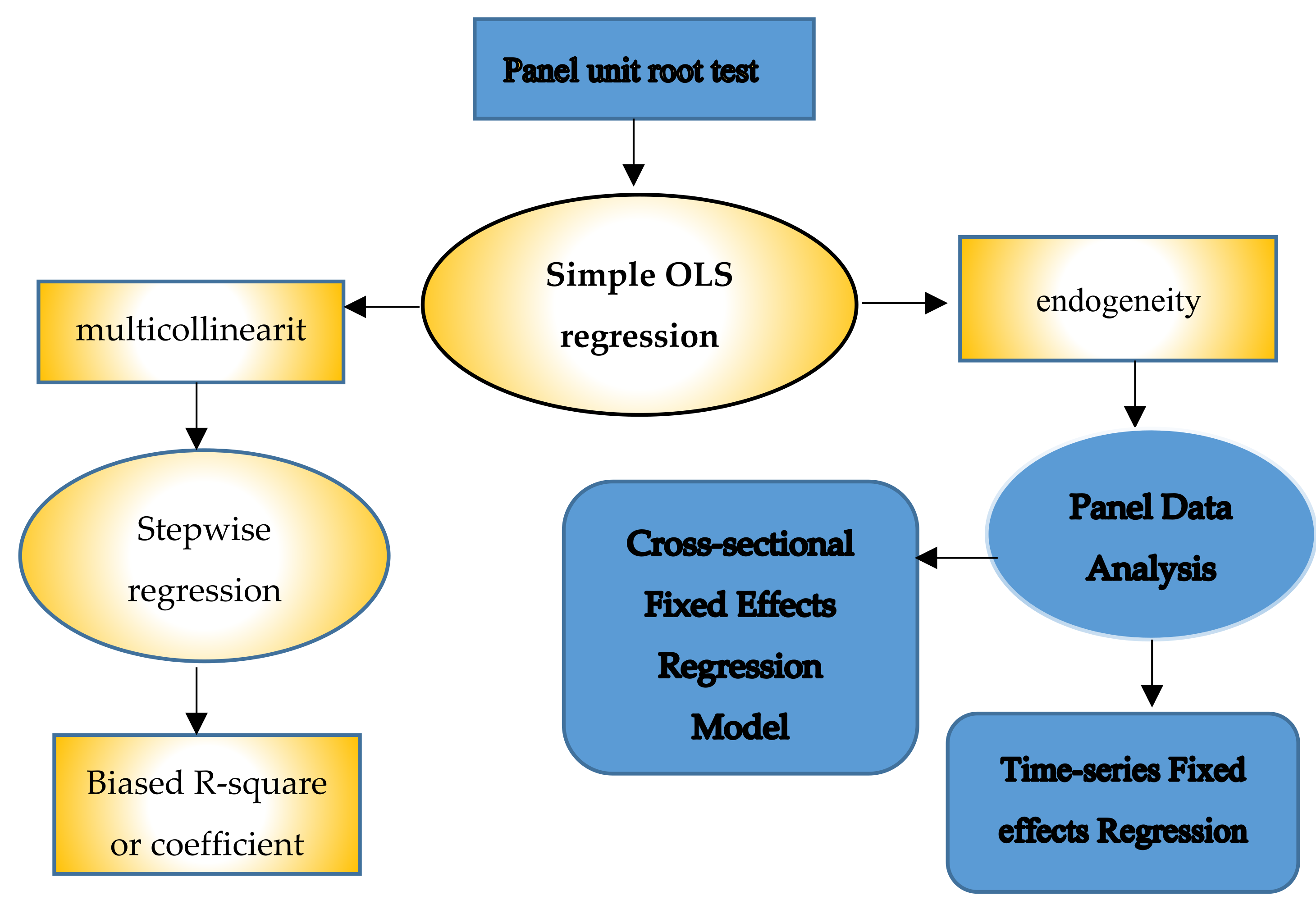
2.2. Study Framework

In order to figure out the association between SWB and EF-related factors to substitute traditional SWB survey, through data observation, a unit root test was initially conducted to make sure variables pass the test, then a simple OLS regression model and detect t-test were conducted. Multicollinearity and endogeneity were found out as the reasons without passing the t-test. Facing multicollinearity, stepwise regression was set forth, and the results showed biased R-square. Facing endogeneity, a fixed-effects panel regression model in cross-section and time-series was elucidated, respectively. The modeling framework in Figure 1 is as follows.

2.3. Methods

2.3.1. Panel Unit Root Test

Panel unit root test is the common feature of panel data analysis. The early panel unit root test meant Dickey-Fuller (ADF) tests, the Phillips-Perron tests, and the Iwiatkowski et al. (1992) tests [40]. The first-generation panel unit root test is called the Levin-Lin-Chu (LLC) [41]. Im-Pesaran-Shin [42] and the Hadri [43] are the second-generation panel unit root tests. They minimized the size distortions and increased the power. A theoretical description of these tests is presented as follows: The data-producing process of the series y, in its different form, be:
Δ y _ i t = α y i t 1 + j = 1 p i β i j Δ y i t j + X δ + ε i t
where i = 1 ,   2 ,   3 ,   ,   N representing cross-sections and t = 1 ,   2 ,   3 ,   ,   T meaning period observations, X _ i t are the exogenous variables such as individual effects and linear trends, α = ρ 1 and ρ _ i are the autoregressive coefficients. The LLC assumes that the autoregressive coefficients in (2) are identical across the panel (common unit root process), while in the IPS test, they are different. In the LLC test, the null hypothesis is the presence of a unit root for all i , and the alternative hypothesis requires that the individual process is stationary for all i , and when the null hypothesis is the same, the alternative in the IPS test is illustrated to include a non-zero fraction of individual process as stationary. IPS statistic equation as:
t _ I P S = N t ¯ 1 N i = 1 N E [ t i T | ρ i = 0 ] 1 N i = 1 N V a r [ t i T | ρ i = 0 ]
In Equation (2), according to the simple Lindberg-Levy theory, the test statistic is asymptotically distributed as N (0,1) as the number of observations is extremely large. Im et al. (2003) exhibited values of the mean and variance for standardizing the test statistic [44].

2.3.2. Stepwise Regression (SR)

SR is an automatic variable selection procedure that selects from a couple of candidates the explanatory variables, which are the most related. We used the unidirectional forward methods. Forward selection begins with no variables in the model, examining each variable with a chosen model-fit criterion until none of the remaining variables improves the model to a statistically significant extent [45].

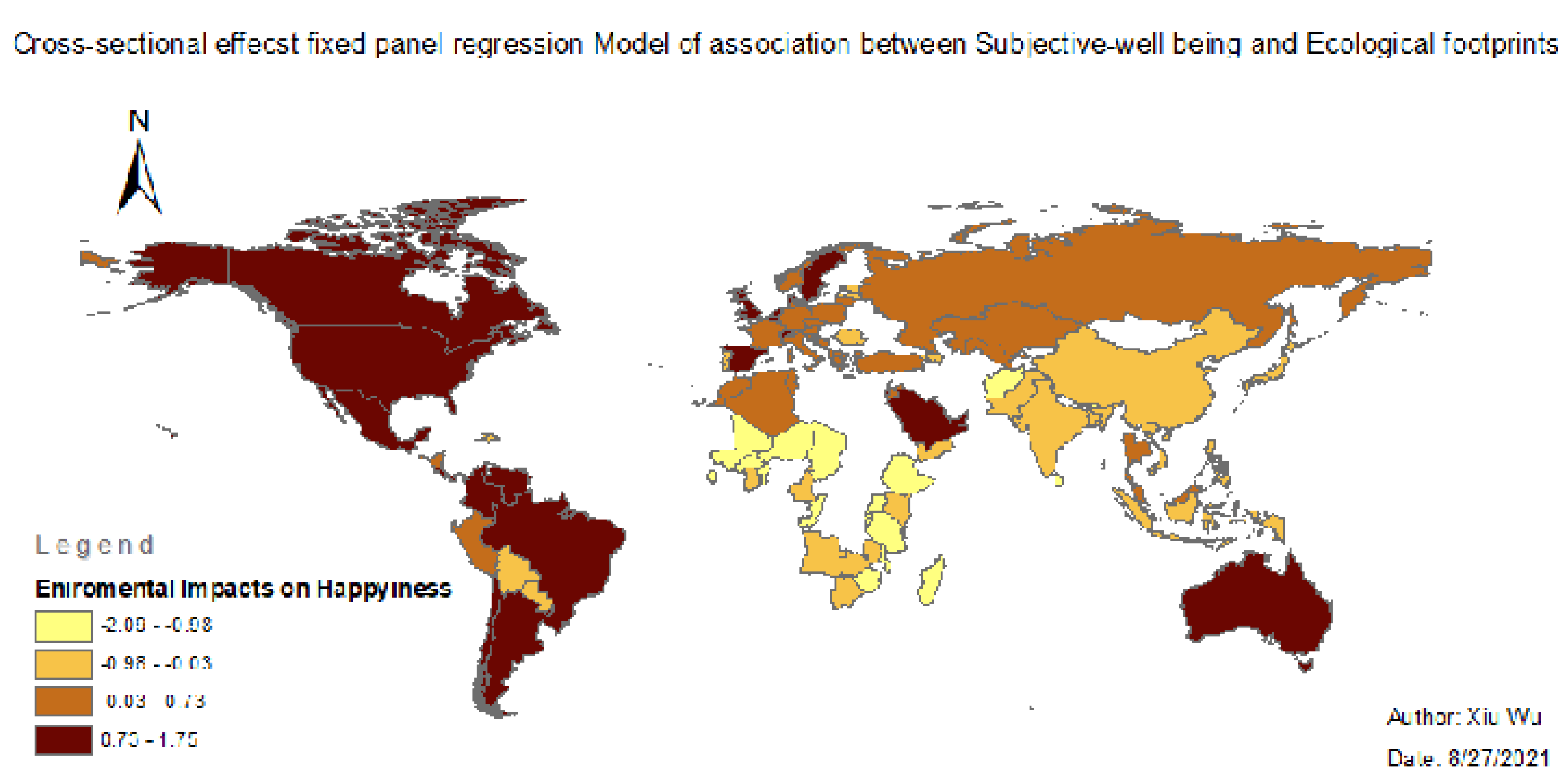
2.3.3. Fixed Effect Panel Model

In order to eliminate the endogenous or exogenous problems, we investigated panel data regression models based on previous research of partial correlations [8]. Panel data typically mean “data containing time series observations of a number of individuals” [46]. They contain independently pooled panels, random-effects models, and fixed effects models. Fixed effects panel regression models (FEPR) have two-dimensional data, referring to cross-sectional fixed effects models and longitudinal fixed-effects models. It is a widespread regression model in macros spectrum analysis due to the impact disparity of spatio-temporal heterogeneity. Panel data have many strengths in either cross-sectional or time-series data, including: (1) more accurate model parameters; (2) more widely available in the international spectrum; (3) more intensive capacity for collecting the complication of human behavior than a single angle; (4) more simplified computation and statistical inference (Hsiao, 2007); (5) minimize the effects of aggregation bias, from aggregating firms into large scale; (6) better measure the impacts that can be detected in neither cross-section nor time-series data; (7) more reliable estimates and test more sophisticated behavioral models with less restrictive assumptions; (8) control for individual heterogeneity [47,48].
The below equation is used to model SWB on various dimensions of EF.
S W B i t = β 0 i + β 1 i × E F s i + β 2 i × C o n t r o l s i + u i t
where the dependent variable SWB is the subjective well-being level for country i in year t. The explanatory variables EFsi are a set of environmental indices, which measure the different types of resources consumption including EF, BC, CBF, CLF, FIF, BLF, GLF, and FLF. C o n t r o l s i are variables that may relatively affect SWB including GDP, URB, WSW, LR, YLE, PS, and VA. u i t is the disturbance term.

3. Results

3.1. Panel Unit Root Tests

To keep stability-based time-series data and avoid pseudo regression models, unit root tests were emphasized to examine the association between variables. Panel unit root test is a conventional method to examine variable rationality in panel data analysis. The result of panel unit root with SWB variable is shown in Table 1. p-value is 0, qualified cross-section records are 99, observation records are 826 cases. The result of panel unit root of TEF variable of p-value is 0, qualified cross-section records are 99, observation records are 826 cases. The result of panel unit root with TBC variable of p-value is 0.0001, qualified cross-section records are 99, observation records are 826 cases. The result of panel unit root of SWB with control variable of P-value is 0, qualified cross-section records are 4, and observation records are 4655 cases. All variables passed unit root tests owing to p-value less than 0.05.

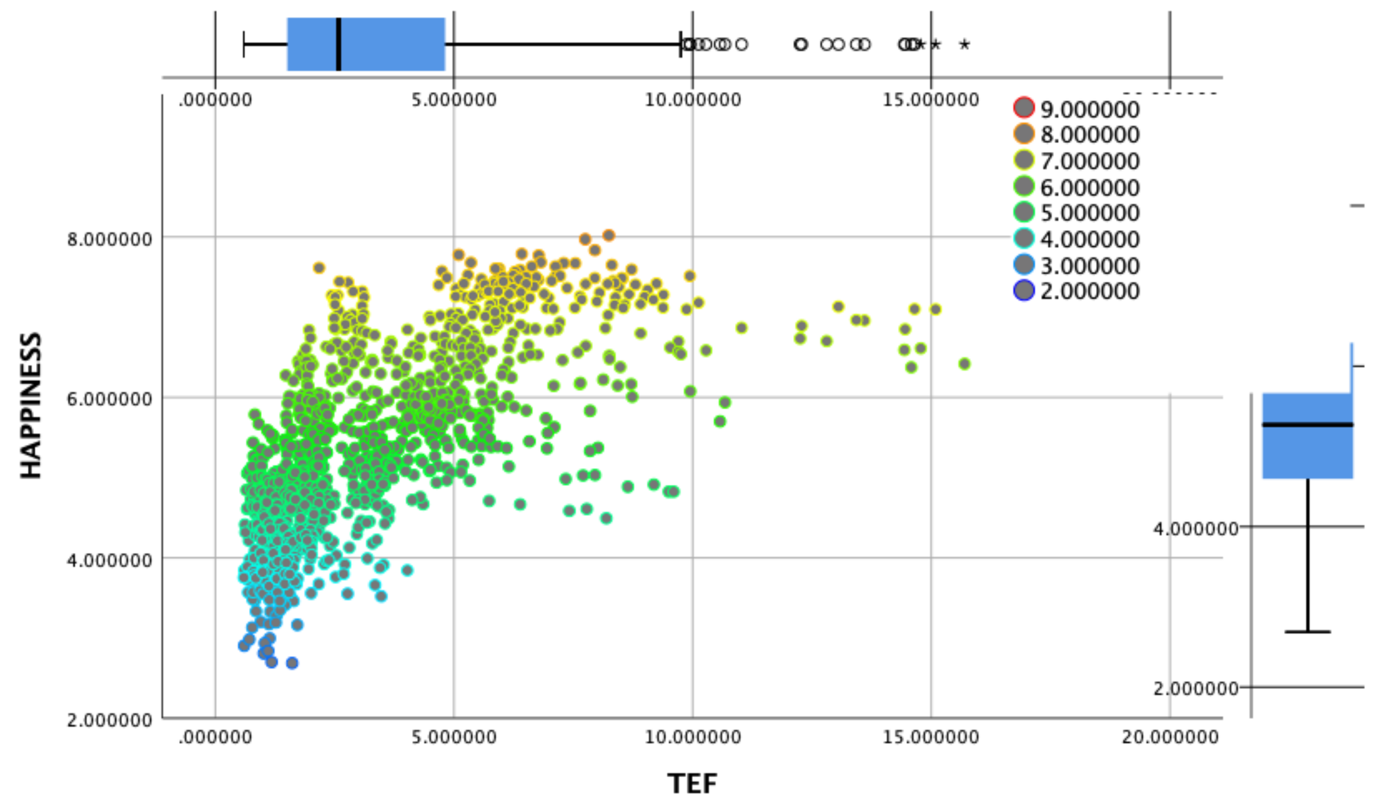
3.2. Regression Analysis

By 965 observation records over a decade, we performed four regression models in Table 2 such as ordinary least square (OLS), stepwise regressions, cross-sectional fixed effects regressions, and time-series fixed effects regressions. In the OLS, we partitioned SWB-control variables OLS (model 1), SWB-EF OLS without control variables (model 2), and SWB-EF OLS with control variables (model 3). The 0.77 R2 of model 3 is higher than others, implying multicollinearity might cause pseudo regressions. The stepwise regression aimed to eliminate multicollinearity negative inventions. Without doubt, EF coefficients were reduced in the step-wise model while the coefficients of control variables were the same as the model 3, including the coefficient of TEF was reduced from −16.17 to −0.026, the coefficient of BLF was reduced from 1.252 to 17.4, the coefficient of CLF was reduced from 0.185 to 16.33, the coefficient of FIF was reduced from −0.22 to 15.93, the coefficient of FLF was reduced from −0.055 to 16.09, the coefficient of GLF was reduced from 0.204 to 16.35.
In the cross-section fixed effects panel regression (model 5) of Table 2, the result shows that BC is negatively related to SWB, based on the coefficient of −0.001, meaning natural supply over time did not impact SWB due to its stationary characteristic, but EF is positive related to SWB due to the coefficient of 0.048, indicating human consumption positively impacts SWB change with time. In particular, the coefficient of BLF was 2.48, the highest value beyond the impacts of control variables and the other explanatory variables, portraying a rise of built-up land consumption in a decade dramatically increased life satisfaction. GLF was positively related to SWB owing to the coefficient of 0.231, depicting grazing-land consumption enhancing people’s happy feelings. Among the control variables, the coefficients of Health, GDP, stability, and education are positive, meaning they have positive impacts on happiness. In other words, an increase in health, GDP, PS, and LR will facilitate more people’s pleasure. In contrast, WSW, VA, and URB have negative coefficients, which means an increase in these coefficients caused losses of people’s safety and indirectly caused SWB shrinking.
Time-series fixed effects panel regression (model 6) of Table 2 is considered spatial disparity without time differencing. The results show that BC is positively related to SWB, based on the coefficient of 0.022, meaning bio-capacity on geographical differences positively increased happiness recognition, but EF is negatively related to SWB due to the coefficient of −0.022, indicating human consumption with spatial heterogeneity inhibits happiness identity. Only interpretation can we imagine that geographical disparity is dominated by culture and religions in a region, and over-sufficient material hedonism induced spirit vacuity. Fixed effect parameters are influenced on discrepancy of geographical location, as shown in Table 3. The coefficients of BLF and GDP (1.611 and 1.56) were the number one and two impacts on SWB spatial dependence, demonstrating that personal spatio-occupation and individual income directly support happiness growth. GLF was positively related to SWB owing to the coefficient of 0.212, which means individual grazing-land consumption can improve people’s happy feelings. Despite the coefficients of WSW and PS are negative, GDP, VA, URB, and LR are positive, meaning their increases will promote more people’s pleasure.
From the time-series fixed effects regression model to the cross-sectional fixed effects regression model, the reliability of the model increased due to an increase in the R-squared value from 0.77 to 0.92. The results also indicated that the stepwise regression model could eliminate multicollinearity. Similarly, Table 2 shows that impacts of cross-section differences in SWB are more striking than time series in several dimensions, including: (1) the effect degree of longitudinal fixed-effects panel regression is in a small range from −0.12 to 0.14, while the effect degree of cross-sectional fixed effects is in a large range from −2.09 to 1.75. (2) R-square values in the longitudinal model are less likely than that in the cross-sectional model (0.77 versus 0.92). (3) Spatial distribution impacts map of cross-section fixed-effects model 5 is exhibited reasonably in different development levels of each country. (4) Time-series fixed effects panel regression model 6 has a low volatility value with different periods of the same countries. (5) Model 6 was not considered a health factor, compared to Model 5.
According to the spatial distribution impacts map of the cross-section fixed effects model, fixed effects in each country are generated in Table 3. We also established a cross-section fixed effects map whose impacts are categorized into five classes with different colors in Figure 2. Green color represents negatively high effects, the values range from −2.09 to −0.98, those countries are distributed in the second-most-populous continent. In these areas, most countries are mainly poor countries with poor health care such as Congo, Niger, and Afghanistan. Tender green colors represent negatively low effects, the values are in the range from −0.98 to −0.03, those countries are distributed in the most populous continent such as Asia. In these areas, most countries are mainly developing countries with fair health care such as China, India, and Mali. The yellow color represents mediate effects. The values are the range from −0.03 to 0.73, those countries are distributed in Europe. In these areas, most countries belong to developed countries with good health care such as France, Germany, and Italy. The red color represents the highest positive effects. The values are in the range from 0.73 to 1.75, those countries are in North America, Europe, and South America. In these areas, most countries belong to the most developed countries with very good health care such as U.S., Denmark, and Sweden. The blue color represents no data.

4. Discussion

According to fixed effects panel regression analysis, the results portrayed that the cross-sectional model was more remarkable than the time-series model. However, in reality, the time-series model is more available than the cross-sectional model in the association between SWB and EF-related factors. First, R-squared values could not determine whether the model is good or not. R-square (R2) is a statistical measure of model fit that indicates how much variation of a dependent variable is explained by the independent variable(s) in a regression model. Indeed, high R-square does not mean good models. In other words, R-square could neither convey the reliability of the model, nor whether the right regression had been chosen. R-square is not a unique standard to examine the reliability of the model. A good model might have a low R-square, a poorly fitted model might have a high R-square, and vice versa. Second, effects values’ range could not determine whether the model is good or not. In the context of the fixed effect models, effects values are constants, which are less important than variables, just like residuals. They just influence the model’s movements but could not change the tendency or directions of the models. Hence, the value of the effects is not a key point when good models or bad models were estimated. Third, correlation coefficients are not reliable in the cross-sectional fixed effects panel regression model. Gehlke and Biehl (1934) argued that correlation coefficients go up with the level of geographic aggregation by census data [49]. In 1950, Robinson found out that the correlation between race and illiteracy increased with the level of geographic aggregation [50]. In other words, what is significant at one spatial scale may not be significant at another. The reason is heteroscedasticity, which is common in spatial regression analysis. Accordingly, correlation coefficients in the cross-sectional fixed effects panel regression model are not available in this research. Last but most importantly, the time-series fixed effects panel regression model supported PC analysis, i.e., SWB is significantly positively related to TBC. In the cross-sectional fixed effects panel regression model (Table 4), SWB has no significant impacts on TBC due to p-value (0.337) beyond 0.05, but SWB has significantly positive impacts on TEF in that coefficient is 0.059 and p-value (0.006) is less than 0.05. On the contrary, in the time-series fixed effects panel regression model, SWB is significantly positively related to TBC for the reason that coefficient is 0.022 and p-value is 0.002, but not significantly related to TEF since coefficient is −0.023 and p-value is 0.143. Hence, it is evident that the time-series fixed effects panel regression model reveals the same result as previous PC analysis.
With respect to the map shown in Figure 2, big disparity of SWB between developed countries and developing countries can be seen. EF has a statistically insignificant impact on the SWB gap, but the economic and demographic structure and GDP growth contribute to the underlying SWB growth. Therefore, environmental improvement is not a determinant of SWB development. However, their correlations might be two folds.
On the one hand, EF is related to individual SWB improvement. For example, we chose 12 countries to represent debtor countries and creditor countries, respectively. In the ranking table of between total EF and EF per capital (Table 5), EF in developed countries is higher than that in developing countries. Resources consumption per person is highly related to the degree of own property. The increasing of the population is the main reason for environmental degradation in developing countries, which leads to low EF producing bad feeling of happiness. In other words, EF might indirectly generate causality with SWB. It probably gets the consequence that individual about environmental improvement benefits individual happiness in a certain time by hedonic treadmill [51], instead, SWB of each country is restricted by multiple factors such as economic and demographic structure, and GDP per capita growth.
On the other hand, even though EF has not had a causality with SWB, EF is an inverted u-shaped link to SWB in correlation analysis using the Weka machine learning in Figure 3. That is in accord with a Kuznets curve, which means environmental improvement has increased from the beginning of SWB growth to a turning point [52,53]. After that, the SWB development benefits environmental degradation with excessive carbon emission, taking up over 60% of TEF [50]. As far as environmental quality increasing, the low-carbon circular economy model might be an underlying, sustainable development trend in future.

5. Conclusions

Within the continuous improvement of the human development index and the popularity of the concept of environmental protection, the low-carbon circular economy model will be an underlying, sustainable development trend to mitigate environment pressure and improve happiness satisfaction from being enforced by the government to people’s subjective consciousness. Space-time fixed effects regression model based on a panel data analysis provided an effective way to study those imbalanced problems.

5.1. Implication

This research provided an underlying quantitative method to measure SWB using socio-economic and environmental impact factors. It not only compensates weakness of qualitative SWB research but also sets forth the feasibility of model-dominated SWB calculation. Because the shortcoming of SWB calculation endows weights to partition ranks from 1 to 10 [54], the fixed-effect model is a supplement through regression analysis, especially missing data in qualitative research. Besides, with increasing environmental awareness and government emission policies, shrinking EF targets carbon emission reduction and end-of-life products supply [55]. This research provides public and transparent platform for exploring carbon-footprint tracking and carbon balance [56]. Resource scarcity is a common tendency around the globe so that circular economy [57] and zero-waste policy is not a surprise for environmental austerity consideration at the local government level. Lastly, a circular economy is just as important for a healthy environment as the balance of natural supply and demand. Nevertheless, the traditional linear model that resources are extracted from the nature and eventually discarded as waste to landfill, caused resource overconsumption and hampered environmental sustainability [58]. A circular economy aims to move away from the model in the context of stretching the life of material resources while minimizing pressures to ensure environmental benefits [59]. This research gave data-driven support in favor of circular economy.

5.2. Limitation

This paper just addressed the model-based interpretation of environmental, political, social-economic impacts on SWB, and there are still unperfect considerations to be improved. First, some essential culture-related factors should be encompassed in the model, such as religion, social media, the tradition of wisdom, and tourism [60,61,62,63,64,65]. Sometimes those entities predominate developed countries or undeveloped countries in intangible or tangible stimulations of human life. Second, the model presents different ways without fixed equations and coefficients, showing that the model has more potential requirements to be improved in the future. EF concept himself should offer detailed components in terms of structures. For example, carbon footprint takes up beyond 70% of total footprints, which disguise the influence of other footprints, especially built-up land sprawls due to global urbanization overwhelming. Lastly, environmental impacts on SWB need an unfolded process, thus, it is important to draw attention to individual EF in our daily lifestyle. Future research of calculating individual EF impacts should focus on the ecological research agenda.

Supplementary Materials

The following are available online at https://www.mdpi.com/article/10.3390/land10090931/s1, Table S1: Variable abbreviation list.

Author Contributions

Conceptualization, X.W. and J.Z.; methodology, X.W.; software, J.Z.; validation, X.W., J.Z., and D.Z.; formal analysis, X.W.; investigation, X.W.; resources, J.Z.; data curation, X.W.; writing—original draft preparation, X.W.; writing—review and editing, J.Z.; visualization, J.Z.; supervision, D.Z.; project administration, J.Z. All authors have read and agreed to the published version of the manuscript.

Funding

This research received no external funding.

Institutional Review Board Statement

Not applicable.

Informed Consent Statement

Not applicable.

Data Availability Statement

All data, models, and code generated or used during the study appear in the submitted article.

Acknowledgments

I would like to extend my sincere gratitude to my advisor, F. Benjamin Zhan, for his instructive advice and useful suggestions on this paper.

Conflicts of Interest

The authors declare no conflict of interest.

References

  1. IPCC. IPCC special report on the ocean and cryosphere in a changing climate. In Intergovernmental Panel on Climate Change; World Meteorological Organization: Geneva, Switzerland, 2019; Available online: https://www.ipcc.ch/srocc/ (accessed on 31 August 2021).
  2. Zhang, J.; Wu, X.; Chow, T.E. Space-Time Cluster’s Detection and Geographical Weighted Regression Analysis of COVID-19 Mortality on Texas Counties. Int. J. Environ. Res. Public Health 2021, 18, 5541. [Google Scholar] [CrossRef]
  3. Strack, F.; Argyle, M.; Schwarz, N. Subjective Well-Being: An Interdisciplinary Perspective, 1st ed.; Pergamon Press: London, UK, 1991. [Google Scholar]
  4. Diener, E.; Tay, L. Subjective Well-Being and Human Welfare around the World as Reflected in the Gallup World Poll. Available online: http://libproxy.txstate.edu/login?url=http://search.ebscohost.com/login.aspx?direct=true&db=s3h&AN=101190444&site=eds-live&scope=site (accessed on 31 August 2021).
  5. Sharif, S.P.; Amiri, M.; Allen, K.-A.; Nia, H.S.; Fomani, F.K.; Matbue, Y.H.; Goudarzian, A.H.; Arefi, S.; Yaghoobzadeh, A.; Waheed, H. Attachment: The mediating role of hope, religiosity, and life satisfaction in older adults. Health Qual. Life Outcomes 2021, 19, 57. [Google Scholar] [CrossRef]
  6. Hui, V.; Constantino, R.E. The association between life satisfaction, emotional support, and perceived health among women who experienced intimate Partner violence (IPV)—2007 behavioral risk factor surveillance system. BMC Public Health 2021, 21, 641. [Google Scholar] [CrossRef]
  7. Richter, N.; Bondü, R.; Trommsdorff, G. Linking transition to motherhood to parenting, children’s emotion regulation, and life satisfaction: A longitudinal study. J. Fam. Psychol. 2021. [Google Scholar] [CrossRef] [PubMed]
  8. Zhang, J.; Zhan, F.; Wu, X.; Zhang, D. Partial Correlation Analysis of Association between Subjective Well-Being and Ecological Footprint. Sustainability 2021, 13, 1033. [Google Scholar] [CrossRef]
  9. Zhang, Z.; Zhang, J. Perceived residential environment of neighborhood and subjective well-being among the elderly in China: A mediating role of sense of community. J. Environ. Psychol. 2017, 51, 82–94. [Google Scholar] [CrossRef] [Green Version]
  10. Charfeddine, L.; Mrabet, Z. The impact of economic development and social-political factors on ecological footprint: A panel data analysis for 15 MENA countries. Renew. Sustain. Energy Rev. 2017, 76, 138–154. [Google Scholar] [CrossRef]
  11. York, R.; A Rosa, E.; Dietz, T. STIRPAT, IPAT and ImPACT: Analytic tools for unpacking the driving forces of environmental impacts. Ecol. Econ. 2003, 46, 351–365. [Google Scholar] [CrossRef]
  12. Graham, C. Happiness And Health: Lessons—And Questions—For Public Policy. Health Aff. 2008, 27, 72–87. [Google Scholar] [CrossRef] [Green Version]
  13. Lin, D.; Hanscom, L.; Murthy, A.; Galli, A.; Evans, M.; Neill, E.; Mancini, M.S.; Martindill, J.; Medouar, F.-Z.; Huang, S.; et al. Ecological Footprint Accounting for Countries: Updates and Results of the National Footprint Accounts, 2012–2018. Resources 2018, 7, 58. [Google Scholar] [CrossRef] [Green Version]
  14. Liu, X.; Li, L.; Ge, J.; Tang, D.; Zhao, S. Spatial Spillover Effects of Environmental Regulations on China’s Haze Pollution Based on Static and Dynamic Spatial Panel Data Models. Pol. J. Environ. Stud. 2019, 28, 2231–2241. [Google Scholar] [CrossRef]
  15. Magdoff, F.; Foster, J.B.; Buttel, F.H. Hungry for Profit: The Agribusiness Threat to Farmers, Food, and the Environment; Monthly Review Press: New York, NY, USA, 2020. [Google Scholar]
  16. Guo, S.; Wang, Y. Ecological Security Assessment Based on Ecological Footprint Approach in Hulunbeir Grassland, China. Int. J. Environ. Res. Public Health 2019, 16, 4805. [Google Scholar] [CrossRef] [Green Version]
  17. Destek, M.A.; Ulucak, R.; Dogan, E. Analyzing the environmental Kuznets curve for the EU countries: The role of ecological footprint. Environ. Sci. Pollut. Res. Int. 2018, 25, 29387–29396. [Google Scholar] [CrossRef] [PubMed]
  18. Rees, W.; Wackernagel, M. Urban Ecological Footprints: Why Cities Cannot Be Sustainable—And Why They Are a Key to Sustainability; Elsevier Science Inc.: Amsterdam, The Netherlands, 1996. [Google Scholar] [CrossRef]
  19. Hori, S.; Takamura, Y.; Fujita, T.; Kanie, N. International Development and the Environment: Social Consensus and Cooperative Measures for Sustainability; Springer: New York, NY, USA, 2020. [Google Scholar]
  20. Easterlin, R.A. Does Economic Growth Improve the Human Lot? Some Empirical Evidence. In Nations and Households in Economic Growth; Academic Press: Cambridge, MA, USA, 1974; pp. 89–125. [Google Scholar]
  21. Stelzner, M. Growth, Consumption, and Happiness: Modeling the Easterlin Paradox. J. Happiness Stud. 2021, 2021, 1–13. [Google Scholar] [CrossRef]
  22. Panayotou, T. Empirical Tests and Policy Analysis of Environmental Degradation at Different Stages of Economic Development. 1994. Available online: http://libproxy.txstate.edu/login?url=http://search.ebscohost.com/login.aspx?direct=true&db=edselc&AN=edselc.2-52.0-0028443307&site=eds-live&scope=site (accessed on 31 August 2021).
  23. Sassen, S. The Global City: New York, London, Tokyo, 2nd ed.; Princeton University Press: Princeton, NJ, USA, 2001; Available online: http://libproxy.txstate.edu/login?url=http://search.ebscohost.com/login.aspx?direct=true&db=cat00022a&AN=txi.b2414811&site=eds-live&scope=site or http://libproxy.txstate.edu/login?url=https://ebookcentral.proquest.com/lib/txstate/detail.action?docID=1144732; (accessed on 31 August 2021). [Google Scholar]
  24. Sarkodie, S.A. Environmental performance, biocapacity, carbon & ecological footprint of nations: Drivers, trends and mitigation options. Sci. Total. Environ. 2021, 751, 141912. [Google Scholar] [CrossRef]
  25. Dietz, T.; Rosa, E.A.; York, R. Environmentally efficient well-being: Rethinking sustainability as the relationship between human well-being and environmental impacts. Hum. Ecol. Rev. 2009, 16, 114–123. [Google Scholar]
  26. Easterlin, R.A.; Sawangfa, O. Happiness and economic growth: Does the cross section predict time trends? Evidence from developing countries. In International Differences in Well-Being; Diener, H., John, F., Kahneman, D., Eds.; Oxford University Press: New York, NY, USA, 2009; pp. 166–216. [Google Scholar]
  27. Fan, Y.; Liu, L.-C.; Wu, G.; Wei, Y.-M. Analyzing impact factors of CO2 emissions using the STIRPAT model. Environ. Impact Assess. Rev. 2006, 26, 377–395. [Google Scholar] [CrossRef]
  28. Fang, K. Ecological footprint depth and size: New indicators for a 3D model. Acta Ecol. Sin. 2013, 33, 267–274. [Google Scholar] [CrossRef] [Green Version]
  29. Frongillo, E.; Nguyen, H.; Smith, M.D.; Coleman-Jensen, A. Food Insecurity Is Associated with Subjective Well-Being among Individuals from 138 Countries in the 2014 Gallup World Poll. J. Nutr. 2017, 147, 680–687. [Google Scholar] [CrossRef] [Green Version]
  30. Ng, Y.-K. Environmentally Responsible Happy Nation Index: Towards an Internationally Acceptable National Success Indicator. Soc. Indic. Res. 2007, 85, 425–446. [Google Scholar] [CrossRef]
  31. Brusseau, M.L.; Ramirez-Andreotta, M.; Pepper, I.L.; Maximillian, J. Chapter 26—Environmental Impacts on Human Health and Well-Being. Environ. Pollut. Sci. 2019, 477–499. [Google Scholar] [CrossRef]
  32. Evans, G.F.; Soliman, E.Z. Happier countries, longer lives: An ecological study on the relationship between subjective sense of well-being and life expectancy. Glob. Health Promot. 2019, 26, 36–40. [Google Scholar] [CrossRef] [PubMed]
  33. Frey, B.S.; Stutzer, A. Happiness and Economics: How the Economy and Institutions Affect Well-Being; Princeton University Press: Princeton, NJ, USA, 2002. [Google Scholar]
  34. Hassan, S.; Bhuiyan, M.A.H.; Tareq, F.; Doza, B.-; Tanu, S.M.; Rabbani, K.A. Relationship between COVID-19 infection rates and air pollution, geo-meteorological, and social parameters. Environ. Monit. Assess. 2021, 193, 29. [Google Scholar] [CrossRef] [PubMed]
  35. Knight, K.W.; Rosa, E.A. The environmental efficiency of well-being: A cross-national analysis. Soc. Sci. Res. 2011, 40, 931–949. [Google Scholar] [CrossRef]
  36. Prescott-Allen, R. The Well-Being of Nations: A Country-by-Country Index of Quality of Life and the Environment; Island Press: Washington, DC, USA, 2011. [Google Scholar]
  37. Sürücü, A. Predictive Relationships Between Incivility Behaviors Faced by Guidance Counselors and Subjective Well-Being and Life-Domain Satisfaction. Int. J. Progress. Educ. 2021, 17, 17–34. [Google Scholar] [CrossRef]
  38. Chen, R.; Zhang, D.; Li, B. Spatial–temporal calculation simulation of ecological footprint of resource and environmental pollution in green communication. EURASIP J. Wirel. Commun. Netw. 2020, 2020, 1–14. [Google Scholar] [CrossRef]
  39. Lee, L.-F.; Yu, J. Estimation of fixed effects panel regression models with separable and nonseparable space–time filters. J. Econ. 2015, 184, 174–192. [Google Scholar] [CrossRef]
  40. Westerlund, J.; Larsson, R. New tools for understanding the local asymptotic power of panel unit root tests. J. Econ. 2015, 188, 59–93. [Google Scholar] [CrossRef]
  41. Ali, E.B.; Amfo, B. Comparing the values of economic, ecological and population indicators in High- and Low-Income Economies. Econ. Reg. Ekon. Reg. 2021, 17, 72–85. [Google Scholar]
  42. Harris, D.; Harvey, D.I.; Leybourne, S.J.; Sakkas, N. Local Asymptotic Power of the Im-Pesaran-Shin Panel Unit Root Test and the Impact of Initial Observations. Econ. Theory 2009, 26, 311–324. [Google Scholar] [CrossRef] [Green Version]
  43. Hadri, K.; Kurozumi, E.; Yamazaki, D. Synergy between an Improved Covariate Unit Root Test and Cross-sectionally Dependent Panel Data Unit Root Tests. Manch. Sch. 2014, 83, 676–700. [Google Scholar] [CrossRef] [Green Version]
  44. Im, K.S.; Pesaran, M.; Shin, Y. Testing for unit roots in heterogeneous panels. J. Econ. 2003, 115, 53–74. [Google Scholar] [CrossRef]
  45. Guidolin, M.; Pedio, M. Forecasting commodity futures returns with stepwise regressions: Do commodity-specific factors help? Ann. Oper. Res. 2021, 299, 1317–1356. [Google Scholar] [CrossRef]
  46. Hsiao, C. Analysis of Panel Data, 3rd ed.; Cambridge University Press: London, UK, 2014. [Google Scholar]
  47. Mátyás, L.; Sevestre, P. The Econometrics of Panel Data: Fundamentals and Recent Developments in Theory and Practice, 3rd ed.; Springer: New York, NY, USA, 2008. [Google Scholar]
  48. Inglehart, R.; Haerpfer, C.; Moreno, A.; Welzel, C.; Kizilova, K.; Diez-Medrano, J.; Lagos, M.; Norris, P.; Ponarin, E.; Puranen, B.; et al. (Eds.) World Values Survey: Round Six-Country-Pooled Data 2014. Available online: http://www.worldvaluessurvey.org/WVSDocumentationWVL.jsp (accessed on 31 August 2021).
  49. Gehlke, C.E.; Biehl, K. Certain Effects of Grouping Upon the Size of the Correlation Coefficient in Census Tract Material. J. Am. Stat. Assoc. 1934, 29, 169. [Google Scholar] [CrossRef]
  50. Robinson, J. An essay on Marxian economics. Macmillan 1949, 1, 64. [Google Scholar]
  51. Knight, J.; Gunatilaka, R. Income, aspirations and the Hedonic Treadmill in a poor society. J. Econ. Behav. Organ. 2012, 82, 67–81. [Google Scholar] [CrossRef] [Green Version]
  52. Kim, D.-H.; Huang, H.-C.; Lin, S.-C. Kuznets Hypothesis in a Panel of States. Contemp. Econ. Policy 2011, 29, 250–260. [Google Scholar] [CrossRef]
  53. Kong, Y.; Khan, R. To examine environmental pollution by economic growth and their impact in an environmental Kuznets curve (EKC) among developed and developing countries. PLoS ONE 2019, 14, e0209532. [Google Scholar] [CrossRef] [Green Version]
  54. Jammazi, R.; Aloui, C. RETRACTED: On the interplay between energy consumption, economic growth and CO2 emission nexus in the GCC countries: A comparative analysis through wavelet approaches. Renew. Sustain. Energy Rev. 2015, 51, 1737–1751. [Google Scholar] [CrossRef]
  55. Ortiz-Ospina, E.; Roser, M. Happiness and Life Satisfaction. Our World in Data. 2013. Available online: https://ourworldindata.org/happiness-and-life-satisfaction (accessed on 31 August 2021).
  56. Wang, Z.; Wu, Q. Carbon emission reduction and product collection decisions in the closed-loop supply chain with cap-and-trade regulation. Int. J. Prod. Res. 2021, 59, 4359–4383. [Google Scholar] [CrossRef]
  57. McGuire, A.D.; Genet, H.; Zhou, L.; Neal, P.; Sarah, S.; Richard, B.; D’Amore, D.; He, Y.; Rupp, T.S.; Striegl, R.; et al. Assessing historical and projected carbon balance of Alaska: A synthesis of results and policy/management implications. Ecol. Appl. 2018, 28, 1396–1412. [Google Scholar] [CrossRef]
  58. Ghosh, S.K. Circular Economy: Global Perspective; Springer: New York, NY, USA, 2020. [Google Scholar]
  59. Liu, L.; Ramakrishna, S. An Introduction to Circular Economy; Springer: New York, NY, USA, 2021. [Google Scholar]
  60. Ushch-Purii, U. Eudaimonic Happiness as a Convergence Point for Religion and Medicine: The Ukrainian Context. Occas. Pap. Relig. East. Eur. 2021, 41, 106–117. [Google Scholar]
  61. Freitas, D. The Happiness Effect: How Social Media is Driving a Generation to Appear Perfect at Any Cost; Oxford University Press: London, UK, 2017. [Google Scholar]
  62. Giorgino, V. The Pursuit of Happiness and the Traditions of Wisdom; Springer: New York, NY, USA, 2014. [Google Scholar]
  63. Wang, R.; Dai, M.; Ou, Y.; Ma, X. Residents’ happiness of life in rural tourism development. J. Destin. Mark. Manag. 2021, 20, 100612. [Google Scholar] [CrossRef]
  64. Okulicz-Kozaryn, A. Unhappy metropolis (when American city is too big). Cities 2017, 61, 144–155. [Google Scholar] [CrossRef]
  65. Du, P.; Wood, A.; Ditchman, N.; Stephens, B. Life Satisfaction of Downtown High-Rise vs. Suburban Low-Rise Living: A Chicago Case Study. Sustainability 2017, 9, 1052. [Google Scholar] [CrossRef] [Green Version]
Figure 1. Modeling study framework.
Land 10 00931 g001
Figure 2. Cross-sectional fixed effects panel regression model map. Note: The above map was created by ArcMap software from Esri. Co.
Land 10 00931 g002
Figure 3. Correlation Between EF and SWB. Note: Above picture was taken by IBMSPSS Statistics, IBM Corp. Released 2020. IBM SPSS Statistics for Windows, Version 27.0. Armonk, NY, USA: IBM Corp. to the University of Waikato, New Zealand.
Land 10 00931 g003
Table 1. The result of panel unit root of variables.
VariablesMethodCoef.Prob.**Cross-Sections Obs.Records
Null: unit root (assumes common unit root process)
SWBLevin, Lin & Chu t*173.355 0.000 99 826
TEFLevin, Lin & Chu t*−14.698 0.0000 99 826
TBCLevin, Lin & Chu t*−3.793 0.0001 99 826
Control variablesLevin, Lin & Chu t*−19.288 0.0000 4 4651
Null: unit root (assumes individual unit root process)
SWBIm, Pesaran and Shin W-stat −69.319 0.0000 99 826
ADF—Fisher Chi-square 1013.71 0.0000 99 826
PP—Fisher Chi-square 1340.59 0.0001 99 900
TEFIm, Pesaran and Shin W-stat −2.390 0.0084 99 826
ADF—Fisher Chi-square 262.865 0.0014 99 826
PP—Fisher Chi-square 357.207 0.0000 99 900
TBCIm, Pesaran and Shin W-stat −0.054 0.4785 99 826
ADF—Fisher Chi-square 221.116 0.1246 99 826
PP—Fisher Chi-square 387.289 0.0000 99 900
Control variablesIm, Pesaran and Shin W-stat −75.9524 0.0000 4 4655
ADF—Fisher Chi-square 987.895 0.0000 4 4655
PP—Fisher Chi-square 899.930 0.0000 4 4673
** Probabilities for Fisher tests are computed using an asymptotic Chi-square distribution. All other tests assume asymptotic normality. Note: Above data were computed by EViews software that belongs to IHS Global Inc., Englewood, CO, USA.
Table 2. Comparison of four regression models.
Variables
Parameters
OLS OLS OLSStepwise RegressionCross-Sectional Fixed Effects RegressionTime-Series Fixed Effects Regression
Model 1Model 2Model 3Model 4Model 5Model 6
TBC 0.0510.0220.023−0.0010.022
TEF −49.810−16.170−0.0260.048−0.022
BLF 56.19017.4001.2522.1481.611
CBF 50.08016.1500.0000.0000.000
CLF 50.28016.3300.1850.0000.000
FIF 51.28015.930−0.2170.0000.000
FLF 49.67016.090−0.0550.0000.000
GLF 50.17016.3500.2040.2310.212
YLE0.036 0.0390.0390.0110.000
GDP1.370 1.5001.4901.6001.560
PS−0.003 −0.002−0.0020.002−0.002
WSW−0.043 −0.04−0.040−0.041−0.037
VA0.006 0.0050.005−0.0010.004
UBR0.016 0.0140.014−0.0100.014
LR0.007 0.0070.0070.0090.006
C1.2213.9100.9430.9424.1440.852
R20.7590.5750.7710.7700.9220.770
N965.000965.000965.000 965.000965.000
F430.900161.779213.040 91.220154.470
Prob0.0000.0000.000 0.0000.000
Table 3. The effect value of divergent countries in the same period.
COUNTRYEffectCOUNTRYEffectCOUNTRYEffect
Afghanistan−1.51088Lebanon−0.180311Estonia−0.090499
Albania0.045380Lithuania0.277951Ethiopia−1.07871
Angola−0.619248Luxembourg−0.271843France 0.582562
Argentina0.923528Macedonia0.584715Germany 0.586486
Armenia−0.436922Madagascar−1.670047Ghana−0.537327
Australia0.910666Malawi−1.132996Greece 0.429039
Austria0.728967Malaysia0.355872Haiti−0.665673
Azerbaijan−0.466232Mali−1.145177India−0.711663
Bahrain0.101220Mexico1.530931Indonesia−0.036024
Bangladesh−0.689438Montenegro0.389134Israel 1.725349
Belarus0.304442Myanmar−1.222246Italy 0.403465
Belgium0.894801Nepal−1.098227Japan−0.033037
Benin−1.783677Netherlands1.272200Jordan 0.616101
Bhutan−0.976775Nicaragua0.173986Kazakhstan 0.313510
Bolivia−0.13884Niger−1.55483Kenya−0.823037
Bosnia and Herzegovina0.545076Norway0.579930Kuwait 0.156473
Botswana−0.672194Pakistan−0.125697Latvia−0.059265
Brazil1.248360Panama1.219165Sri Lanka−1.253539
Burkina Faso−1.374199Paraguay−0.284495Sweden 1.014358
Burundi−1.96029Peru0.103869Switzerland 0.853278
Cameroon−0.74744Philippines−0.295956Tanzania−1.802745
Canada1.242624Poland0.393796Thailand 0.532577
Chad−1.650706Portugal−0.187612Togo−2.091407
Chile0.925958Romania−0.198973Tunisia 0.163915
China−0.600853Russia 0.320365Turkey 0.259620
Colombia1.101339Rwanda−1.840178Uganda−1.173354
Congo−1.143827S Korea 0.210454United Arab Emirates 0.931038
Costa Rica 1.749141Saudi Arabia 1.125122United Kingdom 0.786135
Croatia 0.286016Serbia 0.236301United States 1.037721
Czech Republic 0.602562Sierra Leone−1.002086Uzbekistan 0.314745
Denmark 1.048223Singapore 0.544174Venezuela 1.414359
Dominican Republic−0.100939Slovenia 0.218718Vietnam−0.472808
El Salvador 0.613418Spain 1.408133Yemen−0.835204
Zimbabwe−1.095074Zambia−0.341393
Note: 101 countries were computed by EViews software that belongs to IHS Global Inc., Englewood, CO, USA https://www.eviews.com/general/about_us.html (accessed on 31 August 2021).
Table 4. Cross-section fixed effects panel regression model.
VariableCoefficientStd. Errort-StatisticProb.
BC−0.0321310.033433−0.9610420.3368
EF0.0591250.0216772.7275210.0065
BLF1.0726070.8264031.2979230.1947
GLF0.0834970.1210510.6897680.4905
VA−0.0017390.001819−0.9559700.3394
UPR−0.0043410.008171−0.5312630.5954
WSW−0.0447850.005499−8.1443630.0000
PS0.0014960.0011181.3381610.1812
GDP6.31 × 10−67.39 × 10−60.8540060.3933
LR0.0034510.0098300.3510460.7256
YLE0.0225980.0100682.2446030.0250
C3.8679090.8595494.4999300.0000
Effects Specification
Cross-section fixed (dummy variables)
Weighted Statistics
R-squared0.964015Mean dependent var7.787289
Adjusted R-squared0.959332S.D. dependent var4.854981
S.E. of regression0.337928Sum squared resid97.40874
F-statistic205.8665Durbin-Watson stat1.621291
Prob (F-statistic)0.000000
Unweighted Statistics
R-squared0.921740Mean dependent var5.498159
Sum squared resid99.34218Durbin-Watson stat1.431227
Note: The above table was created by EViews software that belongs to IHS Global Inc., Englewood, CO, USA https://www.eviews.com/general/about_us.html accessed on 31 August 2021.
Table 5. The ranking between TEF and EF per capital.
CountryDebtor Countries HierarchyCreditor Countries Hierarchy
Total EF
Rank
EF per Capital RankSWB (2017)
Rank
Total EF
Rank
EF per Capital
Rank
SWB (2017)
Rank
China
USA
India16590
Japan 2619
Germany3162133
The U.K.44356
Afghanistan53815
Brazil7421418633
Canada715th last 1st last277
Russia 33273
Australia 41112
Congo Demo 518397
Publisher’s Note: MDPI stays neutral with regard to jurisdictional claims in published maps and institutional affiliations.

