Hydrological Responses to Land Use Land Cover Changes in the Fincha’a Watershed, Ethiopia

Abstract

Land use land cover (LULC) changes are highly pronounced in African countries, as they are characterized by an agriculture-based economy and a rapidly growing population. Understanding how land use/cover changes (LULCC) influence watershed hydrology will enable local governments and policymakers to formulate and implement effective and appropriate response strategies to minimize the undesirable effects of future land use/cover change or modification and sustain the local socio-economic situation. The hydrological response of the Ethiopia Fincha’a watershed to LULCC that happened during 25 years was investigated, comparing the situation in three reference years: 1994, 2004, and 2018. The information was derived from Landsat sensors, respectively Landsat 5 TM, Landsat 7 ETM, and Landsat 8 OLI/TIRS. The various LULC classes were derived via ArcGIS using a supervised classification system, and the accuracy assessment was done using confusion matrixes. For all the years investigated, the overall accuracies and the kappa coefficients were higher than 80%, with 2018 as the more accurate year. The analysis of LULCC revealed that forest decreased by 20.0% between the years 1994–2004, and it decreased by 11.8% in the following period 2004–2018. Such decline in areas covered by forest is correlated to an expansion of cultivated land by 16.4% and 10.81%, respectively. After having evaluated the LULCC at the basin scale, the watershed was divided into 18 sub-watersheds, which contained 176 hydrologic response units (HRUs), having a specific LULC. Accounting for such a detailed subdivision of the Fincha’a watershed, the SWAT model was firstly calibrated and validated on past data, and then applied to infer information on the hydrological response of each HRU on LULCC. The modelling results pointed out a general increase of average water flow, both during dry and wet periods, as a consequence of a shift of land coverage from forest and grass towards settlements and build-up areas. The present analysis pointed out the need of accounting for past and future LULCC in modelling the hydrological responses of rivers at the watershed scale.

1. Introduction

Hydrological modelling and water resource management are highly related to the processes of the hydrologic cycle [1]. This cycle can be affected by land use land cover (LULC) changes, as LULC are an essential component of the terrestrial ecosystem, and have been identified as a change driver worldwide [2]. Indeed, LULC changes (LULCC) can directly influence geomorphologic processes, land productivity, and flora and fauna species [1], with the potential to adversely impact critical ecosystem services [3], foster habitat fragmentation [3], depletion of biodiversity [4,5,6], decreasing land productivity [7,8], and changing climatic conditions [7,8,9,10,11]. Changes in LULC can have both short-term and long-lasting impacts on terrestrial hydrology, altering, for example, the long-term balance between rainfall and evapotranspiration and the resultant runoff [12,13]. Evaluating the past LULC, types of changes, and the forces behind them is paramount to understanding the interrelationships between humans and the natural environment [14,15].

Remote sensing plays an important role in the management of the Earth’s surface by providing spatio-temporal information on LULCC, especially over large [16,17] and poorly monitored areas. LULCC are highly pronounced in developing countries, which are characterized by agriculture-based economies and rapidly increasing populations [18,19]. In those countries, the impact of recent LULCC on biodiversity and human life is evident [20], as well as the need for better evaluating future trends and management strategies to counteract its negative effects. In this sense, assessing the impacts of LULC changes on hydrology remains an important step in watershed management strategies inclusive of water resources planning and conservation measures. In their work, Meyer and Turner [21] discussed that land cover changes are caused by many natural and human driving forces. While the effects of natural causes such as climate change are recognizable over a long period, the effects of human activities are generally more immediate. Population growth causes the degradation of resources that rely on the available land and the interactions and feedbacks between them are very complex and hard to be modelled [22]. People demand land for food production as well as for housing, and in African countries it is a common practice to clear the forest to make farming area and housing. The result of such a practice is that land cover and land use can vary at a quasi-daily scale, following human interventions.

The degree of modification of the natural land cover by human influences, the intensity of the changes, and the location of the LULC within a catchment affect the extent to which the land use determines the hydrological response of a catchment. However, generally, these modifications are evaluated only at the local scale [23], involving difficulties in estimating the contribution of LULCC on the basin-wide hydrological cycle. To overcome such problems, hydrological modelling can be implied. Physically-based hydrological models simulate the spatially distributed streamflow time series, and so they can be used to estimate the relative contributions of land cover changes and climate change/variability at the daily, monthly or even annual time scale [24]. The soil and water assessment tool (SWAT) model has been widely used to assess the effects of LULCC on the hydrological cycle [25,26] and sediment yield [27,28]. Indeed, it represents a cost-effective tool due to its advanced model configuration, which can help in modelling limited data regions and evaluating various scenarios and agriculture management practices [29,30].

The sustainable use of water is becoming increasingly important in the legislative agenda of Ethiopia, as this is one of the developing countries from the world where agriculture is the backbone of the economy, and where agriculture is facing major environmental challenges associated with LULCC [20]. The overall goal of the Ethiopian Water Resources Policy [31] is to enhance and promote all national efforts towards the efficient, equitable, and optimum utilization of the available water resources of the country for significant socio-economic development on a sustainable basis. Therefore, a better understanding of how LULCC influence watershed hydrology will enable local governments and policymakers to formulate and implement effective and appropriate response strategies. In Ethiopia, changes in LULC are also playing a significant role in changing the natural hydrological processes, shifting them towards an increase in surface runoff volumes, an increase in evapotranspiration, and a reduction of infiltration and consequent groundwater recharge [23,32,33,34]. Catching the dynamics of LULC and addressing how they affect the local livelihood is therefore paramount for establishing a sustainable development policy [35,36].

Using the Fincha’a watershed as a case study, the present work (i) reviews past LULC, using three reference years (1994, 2008, 2018), to evaluate the past trends of LULCC as derived from satellite images; (ii) investigates the effects of LULCC on the watershed hydrology, using the SWAT model, to infer a possible relationship between LULC and surface runoff. The first point was addressed via a combination of satellite imagery and geographical information systems. Landsat images of the 3 years were classified using a supervised method, and then the various LULC were compared to derive past trends of change. After an adequate calibration and validation process, the SWAT model was used to evaluate the effect of LULCC on the Fincha’a basin hydrology, pointing out an increase in water discharge due to the loss of forest and grass areas in favour of agricultural and build-up zones.

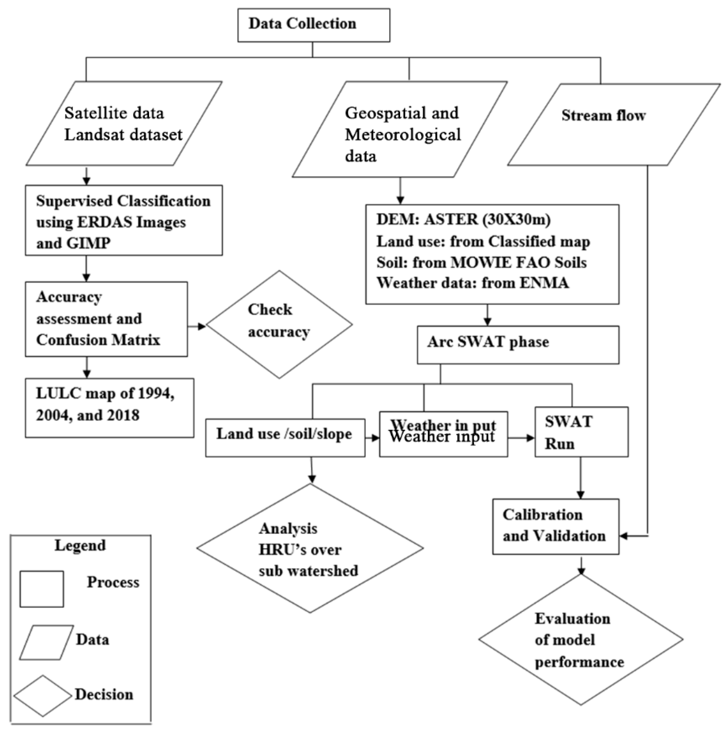
2. Materials and Methods

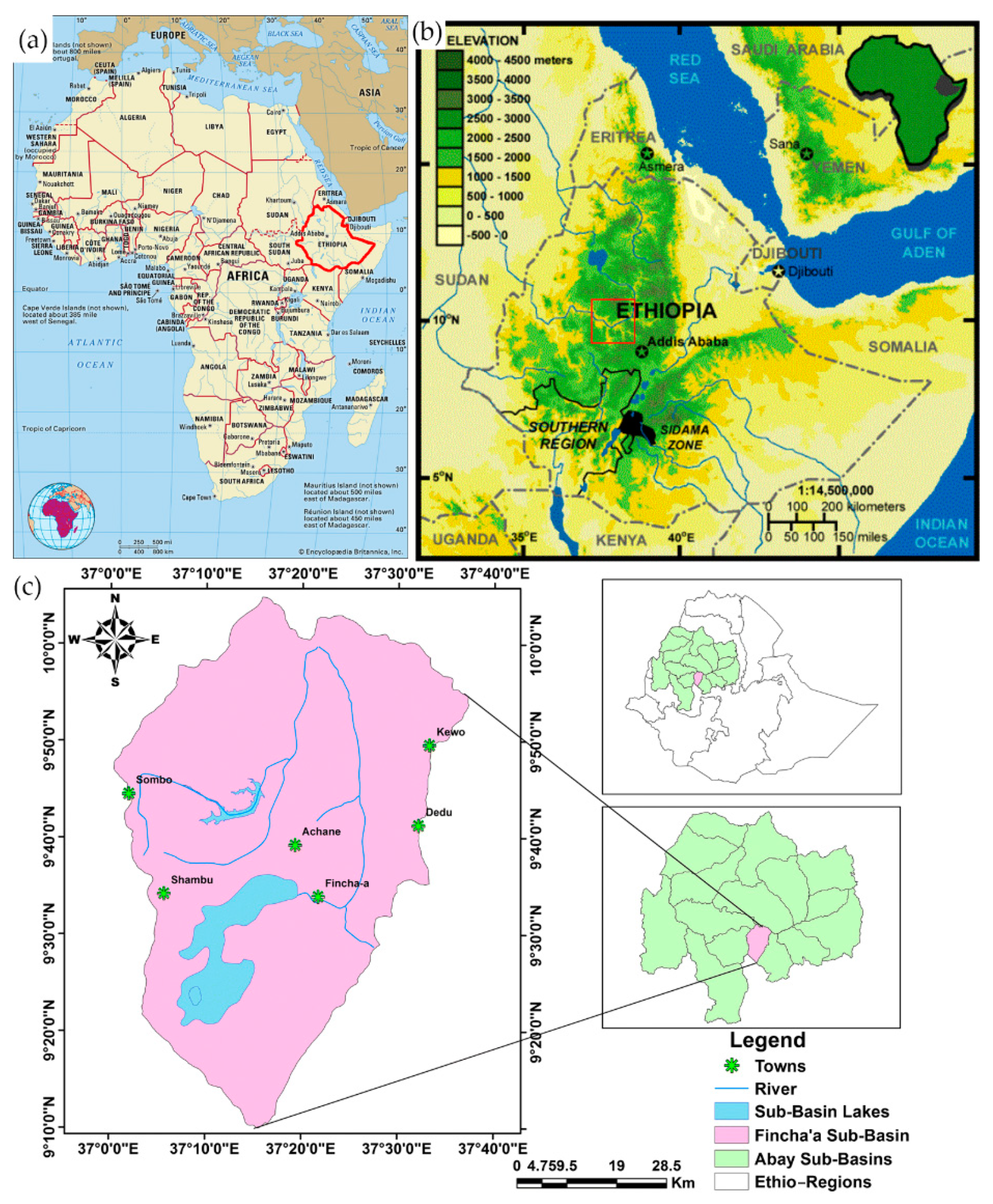
2.1. Study Area

The Fincha’a watershed is part of the Blue Nile basin and is located in the Oromia region, Horro Guduru Wollega zone, Ethiopia, between 9°10′30″ to 9°46′45″ north latitude and between 37°03′00″ to 37°28′30″ east longitude (Figure 1) [37,38]. The watershed is bounded on the south by the Great Gibe River basin, on the north by the Abbay (Blue Nile) River basin, on the west by the Didessa sub-basin, and on the east by the Guder sub-basin. It covers an area of about 3781 km², containing three sub-basins, namely the Fincha’a, Amerti, and Neshe. It covers seven aanaa’s (the Ethiopian second-lowest administrative unit): Abay Chomen, Guduru, Hababo Guduru, Jimma Rare, Horro, Jima Geneti, and Jarte Jardega.

The study followed the workflow presented in Figure 2, and is described in detail in the following sections.

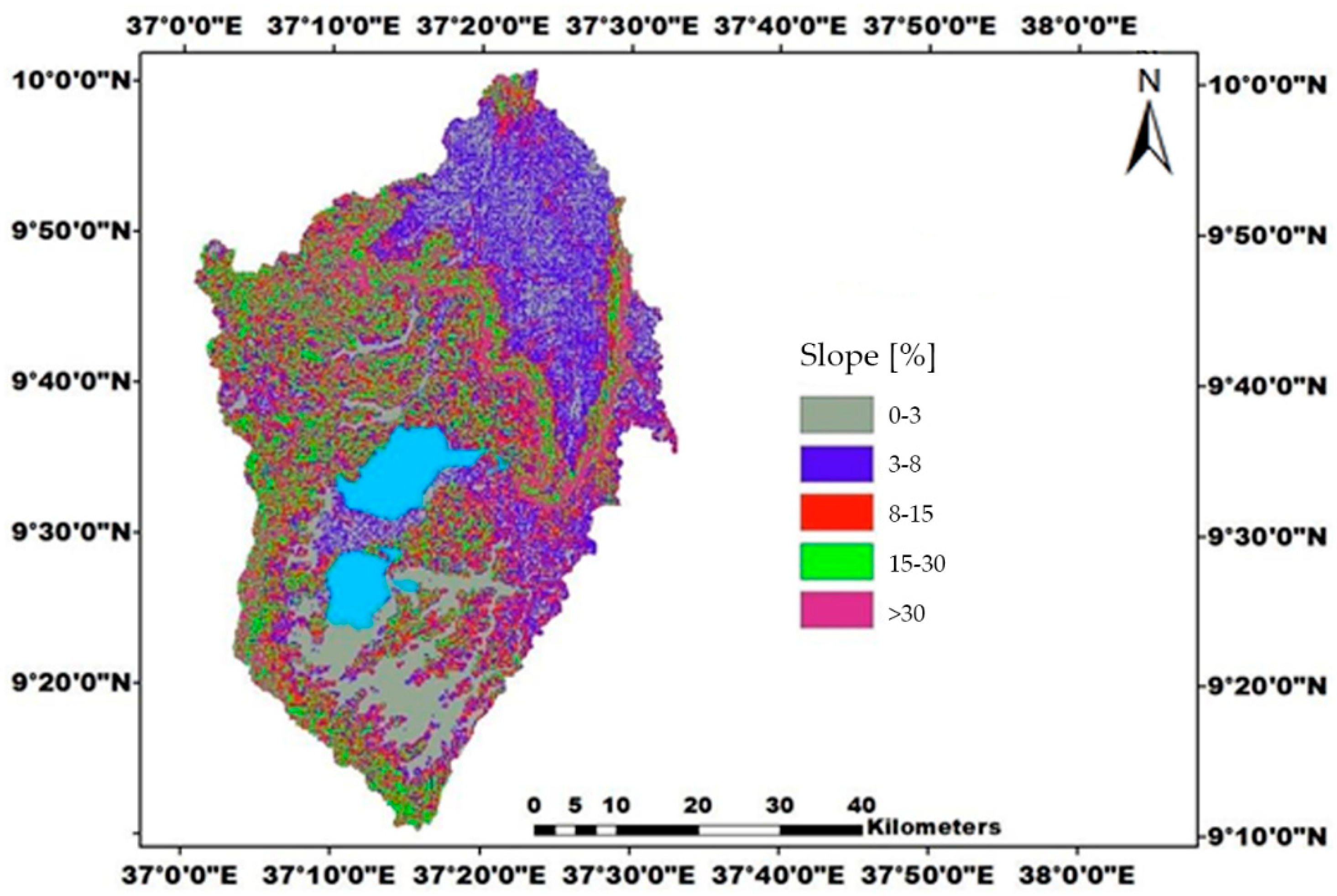
2.1.1. Watershed Topography and Geology

The altitude in the Fincha’a basin ranges approximately between 880 and 3200 m asl. The highlands in the western and southern part of the basin are higher in altitude, greater than 2200 m (Figure 1). The lowlands have a lower altitude, less than 1400 m asl, and are in the northern part.

The dominant soils of the area are clay, loam, and clay-loam, while a small part of the watershed in the northeastern part consists of Adigrat sandstone formation. The higher parts of the watershed near the boundary (where the drainage of all the streams begin) as well as the elevated parts in the middle of the watershed, which are isolated outcrops, are made of Quaternary volcanic [23].

The Fincha’a reservoir is located in the Chomen swamp [39,40], the basin of which is covered with black clay of unknown depth. It may be as much as 10 m deep and is believed to be underlain by volcanic rock. The soil cover forms an excellent impermeable blanket, therefore seepage is not considered to be a serious factor in this area.

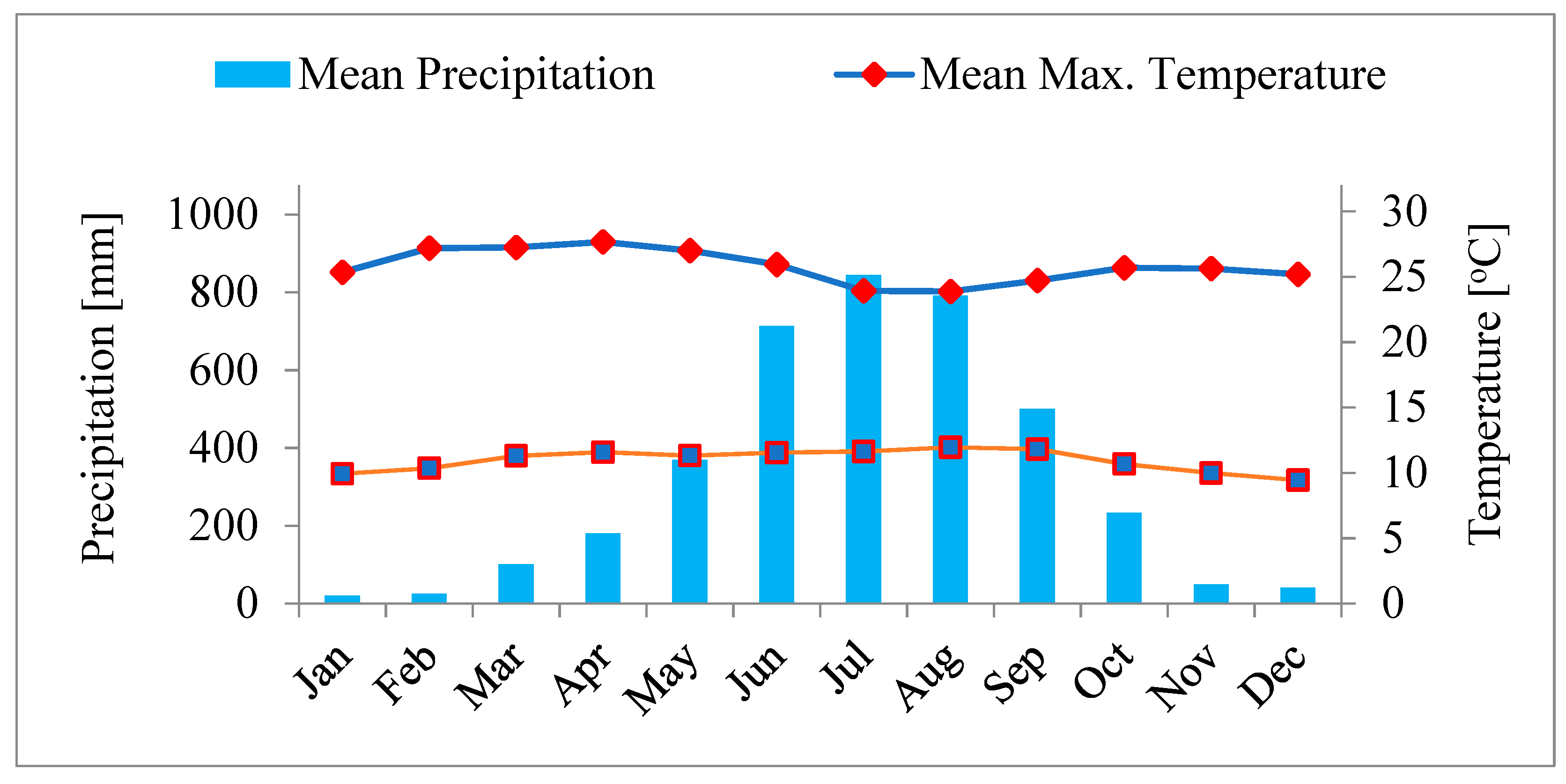
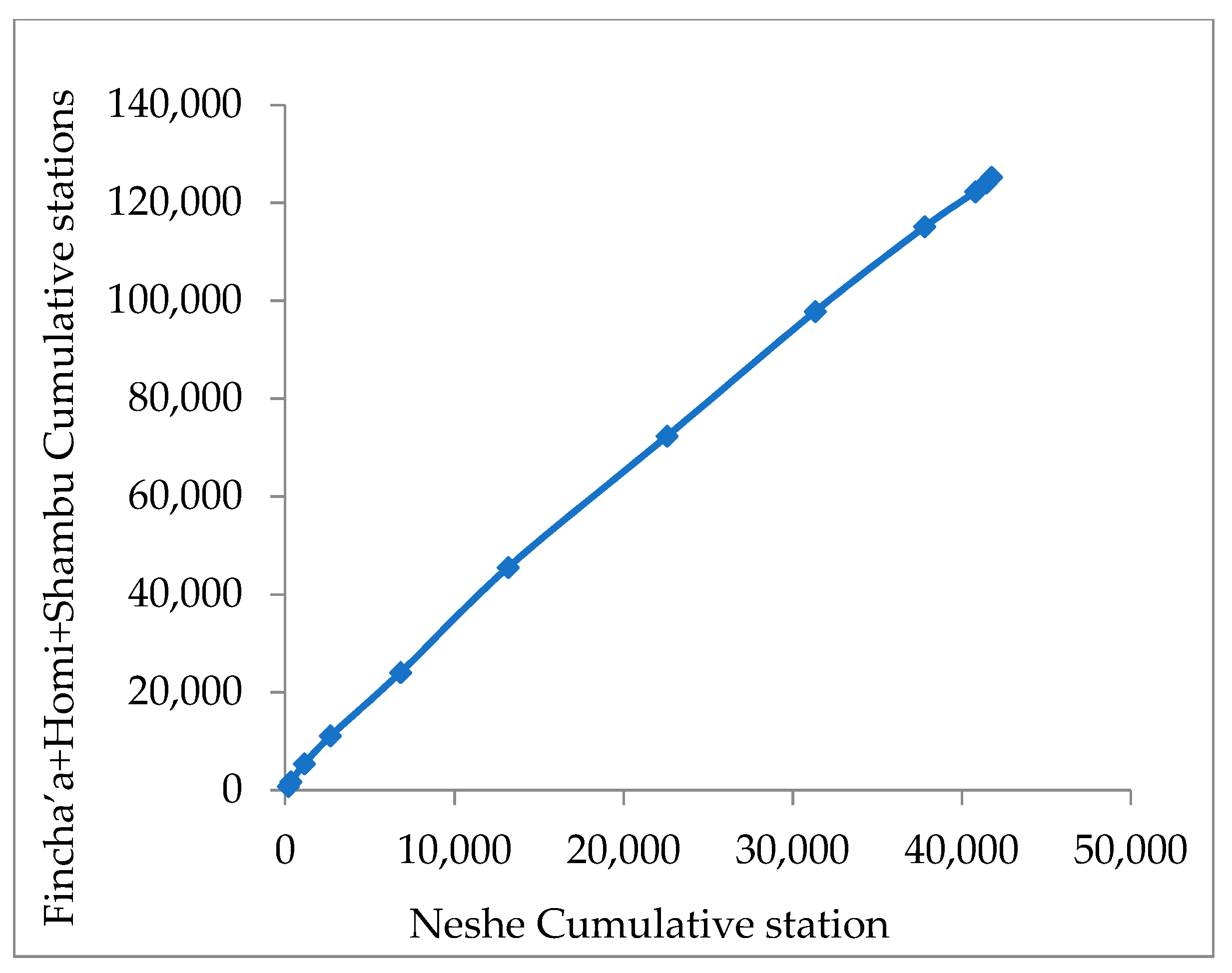
2.1.2. Weather Data

The weather data were collected from the Ethiopian National Metrological Agency (ENMA). Specifically, for the study period, daily data of maximum and minimum temperature, precipitation, relative humidity, wind and solar radiation were collected, referring to four gauging stations: Fincha’a, Homi, Shambu, and Neshe (

Table 1. Meteorological stations of the Fincha’a watershed.

Name	Years of Record	X [°]	Y [°]	Elevation [m asl]
Fincha’a	1989–2018	9.57	37.37	2248
Homi	1987–2018	9.621	37.241	2371
Shambu	1981–2018	9.5712	37.1	2460
Neshe	1981–2018	9.723	37.268	2060

). All the data were combined and prepared to be used as input data for the SWAT model.

Figure 3 summarizes the monthly values of rainfall and temperature in the Fincha’a watershed averaged over the study period. Details on the various parameters are provided in the following subsections.

The daily flow data are required for calibrating the SWAT simulations. These data were obtained from the Ministry of Water, Irrigation, and Energy Office, and post-processed as per the requirement of the modelling tool. The calibration and validation were done on a daily and monthly basis, using the periods 1997–2004 for the calibration and 2005–2008 for validation. Missing and no-data were excluded from this process.

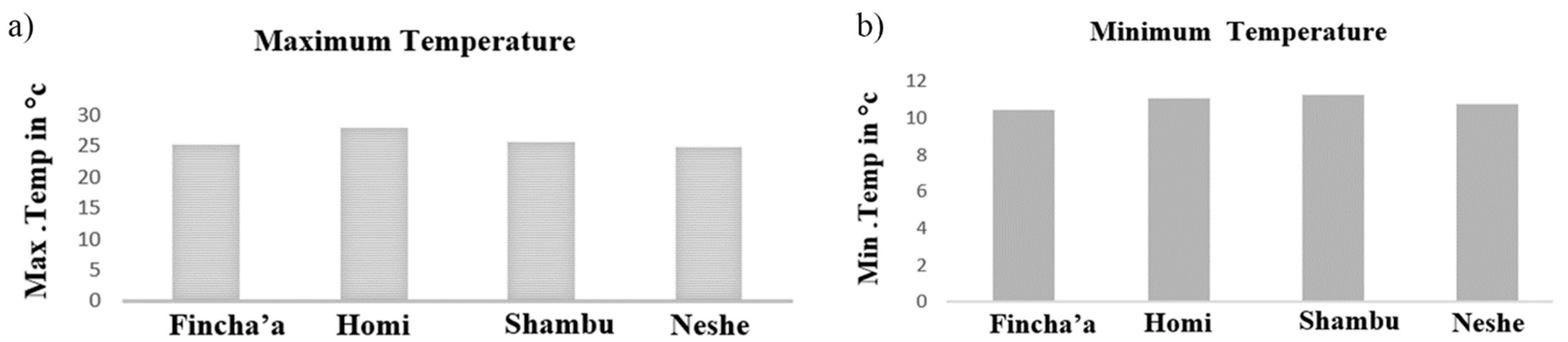
2.1.3. Temperature

The annual minimum and maximum temperatures of the watershed vary from 6.0 to 16.0 °C and from 19.5 to 31.5 °C, with a yearly average of around 10 and 24 °C, respectively (Figure 4), and are the lowest during summer, due to the prevailing cloud cover experienced during this season. During the observed period, the temperature was higher at the Homi metrological gauging station, where a maximum of 27.9 °C was reached during the observed period, while the minimum temperature of 10.4 °C was measured at the Fincha’a metrological gauging station.

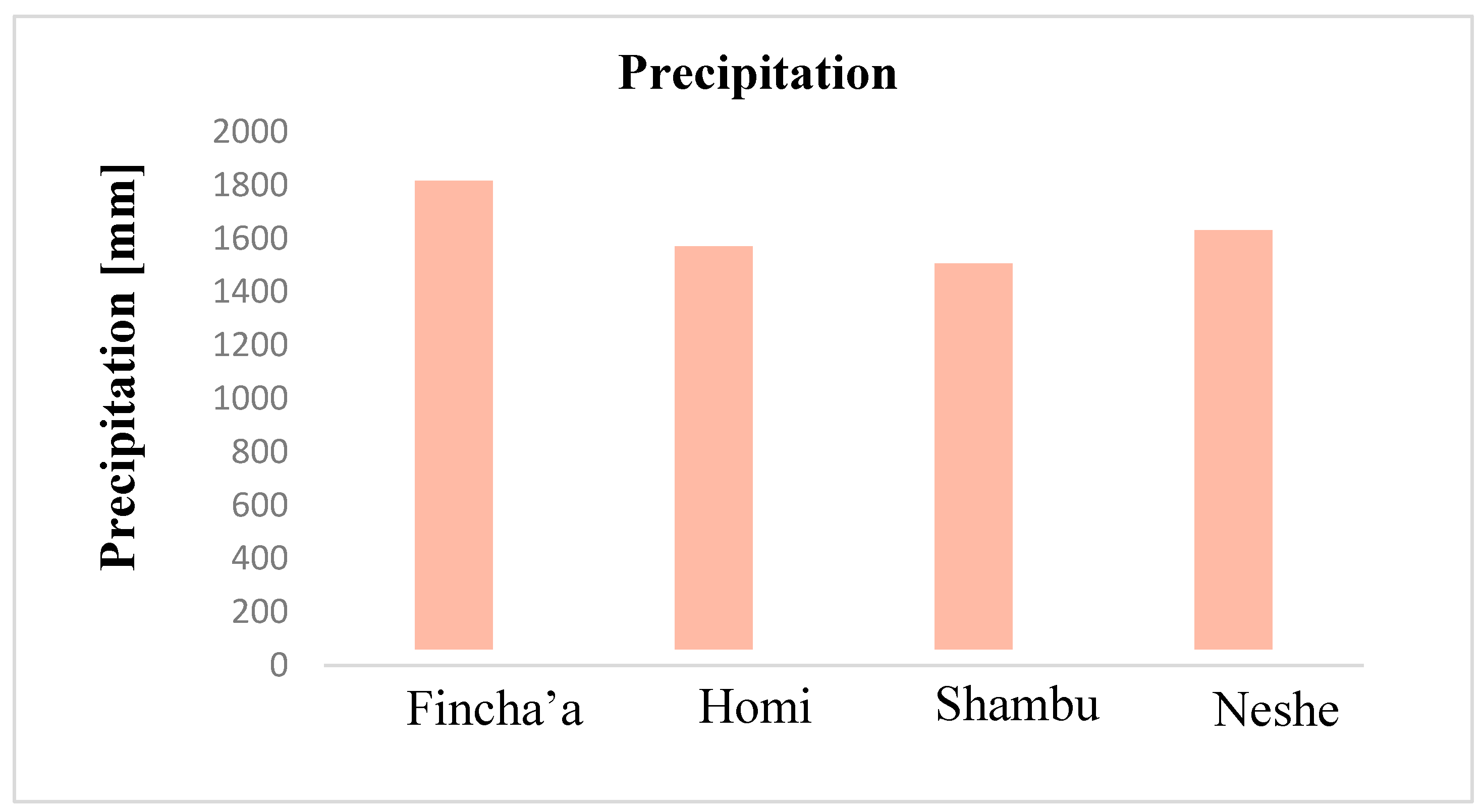
2.1.4. Rainfall

The rainfall data collected from the stations may vary in their qualities and consistencies of record. There are five weather stations in the Fincha’a watershed, but the Hareto station was not used due to the short time record of weather data. The collected data have missing values in all the stations. The missing values in all stations were assigned with no data code (−99), which was then filled by the weather generator embodied in the SWAT model from the monthly weather parameter.

Looking at the long-term statistics of the Fincha’a watershed (see Table 1 for the years of record), the annual rainfall ranges between 960 and 1835 mm. Lower annual rainfall less than 1100 mm was observed in the northern lowlands of the basin and higher rainfall greater than 1300 mm in the western and southern highlands. Generally, the rainfall presents a peak during the summer (July to August) and exhibits minimum values during the winter (December to February). The annual values observed in the four considered stations during the study period vary between 1450 and 1800 mm (Figure 5).

The double mass curve technique was used to check whether the collected rainfall data from the Fincha’a sub-basin meteorological station were consistent through the selected period of study and checked whether corrections were needed or not. A group of certain numbers of neighbouring stations were chosen as base stations from the vicinity of a doubtful station and were considered a doubtful station until checked. The precipitation of station x (doubtful station) can be corrected using Equation (1):

$$P_{cx} = P_x\frac{M_c}{M_a}$$

(1)

where P_cx represents the corrected precipitation at any period t at station X, while P_x is the corresponding original recorded precipitation, and M_c and M_a are the corrected and original slope of the double mass curve, respectively.

A double mass curve was used to investigate whether there was inconsistency for the four considered gauging stations. The records of these stations did not indicate inconsistency, as the graph was found to follow a nearly straight line (Figure 6). This means that all the stations’ data in the Fincha’a watershed were almost consistent.

2.1.5. Evaporation

The potential evapotranspiration (PET) in the basin is generally between 1365 and 1970 mm per year. In the lowlands, a higher temperature is generally observed, driving the PET to values higher than 1800 mm/yr. The highlands in the western and eastern parts of the basin show a lower PET, reaching values of less than 1600 mm/year.

In the upper Fincha’a basin, there are two very large swamps, with the Chomen Swamp being the larger, with a drainage area of about 860 km².

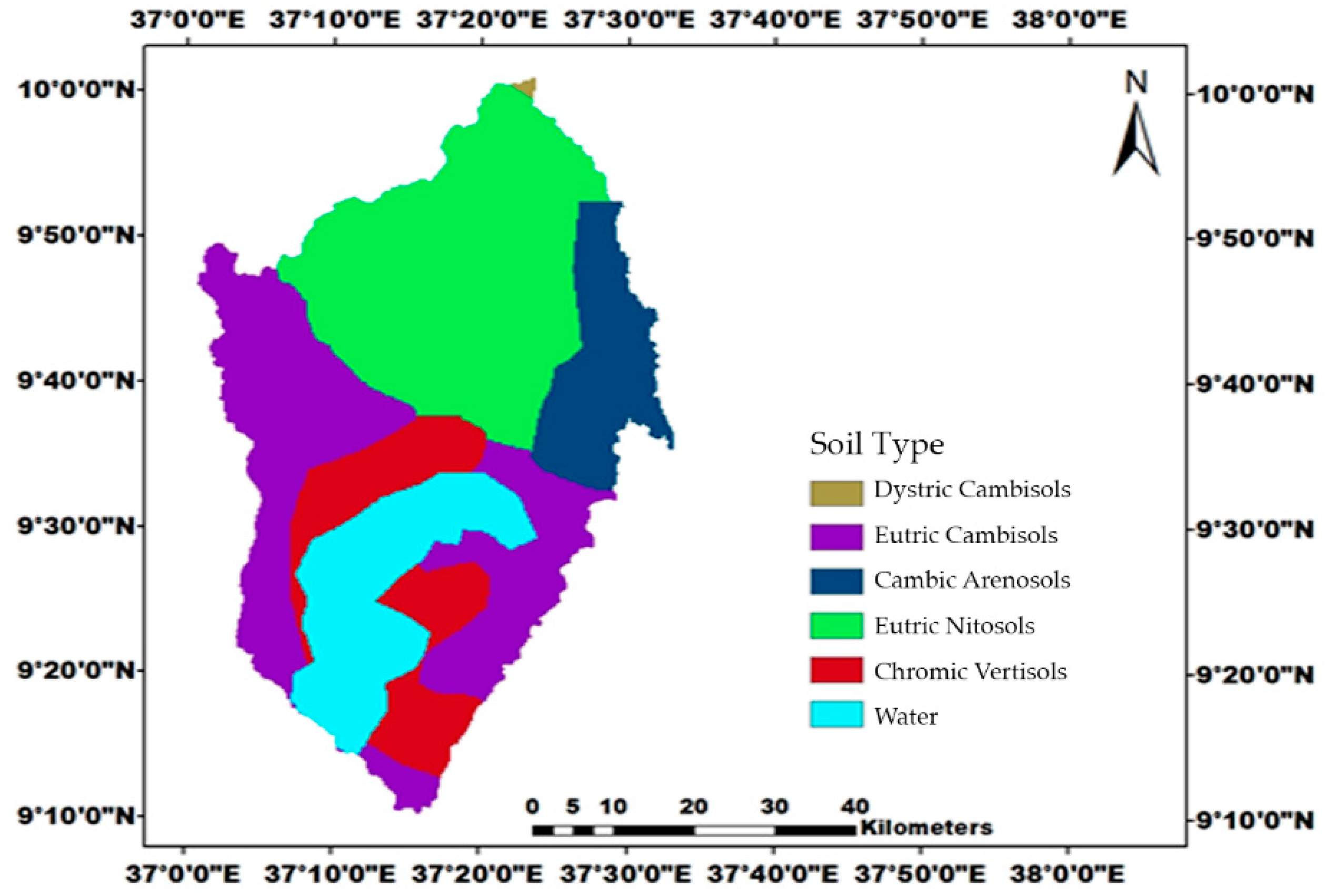
2.1.6. Soil Type

The soil data are a significant component in the study of how LULCC can impact the hydrological components of a watershed. According to a previous study performed by Makin [41], the soil type in the study area is closely related to parent materials, degree of weathering, and the characteristics of the local reliefs. The main parent materials are basalt, ignimbrite, acid lava, volcanic ash, and pumice.

The soil map of the study area was obtained from the Ministry of Water, Irrigation and Electricity of Ethiopia. According to the FAO/UNESCO classification [42], six major soil groups were identified in the Fincha’a watershed: Eutric Nitosols, Eutric Cambisols, Water, Chromic Vertisols, Cambic Arenosols, and Dystric Cambisols (

Table 2. Soils that are present in the Fincha’a watershed.

Soil Name	Area Covered		SWAT Naming
	[ha]	[%]
Dystric Cambisols	437.1643	0.14	Bd31-2c-11
Eutric Cambisols	94,827.3963	29.57	Be8-3c-24
Cambic Arenosols	35,365.7764	11.03	Qc5-1c-182
Eutric Nitosols	113,078.3254	35.27	Ne20-3b-160
Chromic Vertisols	35,579.3598	11.10	Vc23-3a-262
Water	41,360.6536	12.90	WR-192

). In addition to the location of each soil type, the Ministry of Water, Irrigation and Electricity of Ethiopia also provided information about soil physical and chemical properties such as soil texture, available water content, bulk density, hydraulic conductivity, and organic carbon content.

The SWAT model has predefined four-letter codes for each land use category. These codes were therefore used to link or associate the land use map of the study area to the SWAT land-use databases.

Figure 7 shows the soil map of the Fincha’a watershed, pointing out the major presence of Cambric Arenosols in the northern part of the basin, while the southern area is largely covered by water.

2.2. Spatial Data and Satellite Imagery

In addition to information on the local hydrology and soil composition, the present study also requires a digital elevation model (DEM) and satellite images for deriving LULC. This information was derived from multiple sources, such as the Ministry of Water, Irrigation and Energy Resource Office, National Meteorological Agency, and Nile Basin Authority offices.

2.2.1. Digital Elevation Model

For this study, the digital elevation model of the whole Ethiopia (spatial resolution 30 × 30 m) was obtained from the Nile Basin Authority Office, and it was projected to Addenda and UTM Zone 37 to create an overlay with soil and land use raster dataset using Arc-GIS 10.5.1 (Environmental Systems Research Institute, Redlands, CA, USA). The Arc-GIS software was also used to process the DEM and create a triangulated irregular network for deriving both the river network and the flood inundation maps.

2.2.2. Landsat Imagery

Landsat satellite images were analysed to identify changes in land use and land cover distribution in the Fincha’a watershed over 25 years (from 1994 to 2018). For this period, three Landsat images of 1994, 2004, and 2018 were downloaded from the United States Geological Survey website (earthexplorer.usgs.gov) GeoTIFF file format. Landsat thematic mapper (TM), enhanced thematic mapper (ETM), operational land imager (OLI), and thermal infrared sensor (TIRS) were selected to represent the land cover conditions in the years 1994, 2004, and 2018, respectively. Landsat images have a variable spatial resolution, depending on both the sensors and the bands, spanning from 15 to 120 m [43]. For this application, we used images having a spatial resolution of 30 × 30 m, which were geo-referenced to WGS_84 datum and Universal Traverse Mercator (UTM) Zone 37 N. Preprocessing such as layer stacking, mosaicking, and band colour combinations were carried out to orthorectify the images, using the ERDAS Imagine 2014 and GIMP 2.10.12 software.

Table 3. Attributes of Landsat images.

Sensor	Spatial Resolution	Acquisition Date	Image Quality	Path/Row
Landsat 5 TM	30 m	5 January1994	7	169/053
Landsat 7 ETM	30 m	7 December 2004	9	169/053
Landsat 8 OLI/TRIS	30 m	3 December 2018	9	169/053

Source: www.usgs.gov (accessed date 15 March 2021).

reports the details of the used Landsat images.

2.3. Image Classification Process

Image classification is the process of sorting pixels into a finite number of individual classes or categories of data based on their data file values. In remote sensing, there are various image classification methods, such as supervised, unsupervised, and hybrid, as well as innovative methods such as artificial neural networks [44]. Unsupervised classification is computer controlled and its limitation is that the user cannot control the computer’s selection of pixels into clusters. In the case of a supervised image classification system, the user relies on her/his prior knowledge and skills and can select a group of pixels belonging to a particular LULC. In this system, the user is required to have good knowledge about the local conditions of the area under study, or clear field evidence to validate the classification. Supervised classification is the most common type of land use classification system and depends on prior information about the land use and land cover.

Supervised Classification

The present analysis was performed employing the supervised classification method, using previous studies of Bezuayehu [45] and Taye [46] as a reference for classification numbers, as well as the expertise of the scientists involved in the study. No field evidence was specifically collected for this work, due to logistic limits, but the results reported here confirm previous studies [45,46] and unpublished analyses.

Using the Landsat 7 images acquired in 2004, eight classes of LULC such as cultivated land, bare soil, forest land, shrubland, grassland, settlement, waterbody, and wetland were produced (

Table 4. Land use classification of the Fincha’a watershed, and the corresponding SWAT code.

S. No.	Land Use Land Cover	SWAT LULC	SWAT Code
1	Cultivated Land	Agricultural land row crops	AGRR
2	Bare Soil	Barren	BARR
3	Forest Land	Forest-Evergreen	FRSE
4	Shrub Land	Forest-Mixed	FRST
5	Grass Land	Agricultural Land-Generic	AGRL
6	Settlement	Residential	URBN
7	Waterbody	Water	WATR
8	Wetland	Wetlands-Mixed	WETL

):

• Cultivated Land: Areas used for crop cultivation, both annuals and perennials, and the scattered rural settlements that are closely associated with the cultivated fields.
• Bare Soil: Areas covered with soil surfaces and sand with no vegetation cover or uncultivated farmlands consisting of exposed soil and rock outcrops.
• Forest Land: Land covered with dense trees which include evergreen forest land, mixed forest, and sparse trees.
• Shrub Land: Land covered with open shrubs, closed shrubs, bushes, and mixed with small trees.
• Grass Land: Areas covered with grass used for grazing, as well as bare lands that have little grass or no grass cover. It also includes other small-sized plant species.
• Settlement: Area covered with building rural residential houses infrastructures roads.
• Waterbody: Waterlogged areas and lakes throughout the year, the rivers, and their main tributaries.
• Wetlands: An area that is saturated with water, either permanently or seasonally waterlogged around a swamp area.

Since there may be a misclassification of pixels in the supervised classification, it is necessary to test the accuracy of the classification using ground truth, as well as assessing the accuracy via confusions matrixes, as described in Section 3.2.

In fact, a paramount step in the classification process, whether supervised or unsupervised, is the accuracy assessment of the final classification produced. This involves identifying a set of sample locations that have field evidence or using previous studies. The land use and land cover found in the field is then compared to the one mapped in the image for the same location. Then, the statistical assessment of accuracy may be derived for the entire study area. Generally, the accuracy assessment is a very important measurement to determine how accurate the referenced data agree with classified images of the remotely sensed data [47].

The error matrix produced may be used to identify specific cover types for which errors are in excess of that desired. The information in the matrix about which covers are being mistakenly included in a particular class (error of commission) and those that are being mistakenly excluded (errors of omission) from that class can be used to refine the classification approach.

2.4. Hydrological Modelling with SWAT

2.4.1. Model Setup

Arc-SWAT version 2012.10_4.19 was downloaded from the SWAT website (swat.tamu.edu) and its toolbar was added to Arc-GIS 10.5.1 for the modelling process. The modelling procedure includes SWAT project setup, watershed delineation, hydrologic response units (HRU) analysis, write input tables, edit SWAT input, and SWAT simulation. After data collection, all the input data were prepared, the watershed was delineated, the HRUs definition were defined, and the land-use/soil/slope classification was added to the model. The model was run at the basis scale, assuming 3 years of the warm-up period. The details of each step are provided in the following.

2.4.2. Watershed Delineation

The first step in generating a SWAT model is the watershed delineation. The soil map, the LULC map, and the DEM were projected using Arc-GIS 10.5.1 to the same projection system before watershed delineation, to assure maps overlapping. The watershed and sub-watershed delineations were performed using the 30 x 30 m DEM. The obtained slope classes are shown in

Table 5. Slope classes.

Slope	% Area	Area [ha]
0–3	22.5	71,925.8021
3–8	30	95,965.2960
8–15	21	67,548.7056
15–30	18	57,980.1691
>30	8.5	27,228.7031

and Figure 8.

2.4.3. Hydrologic Response Units

After the watershed delineation, land use, soil, and slope characterization were performed using commands from the HRU analysis menu on the Arc-SWAT toolbar. These tools were used in loading land use and soil layers of the Fincha’a watershed into the current project, to evaluate the slope characteristics and determine the land use/soil/slope class combinations and distributions for each sub-basin.

The SWAT user’s manual suggests that a 20% land use threshold, 10% soil threshold, and 20% slope threshold are adequate for the most common modelling applications. However, Setegn et al. [48] suggested that the HRU definition with multiple options that account for 10% land use, 20% soil, and 10% slope threshold combinations gives a better estimation of runoff and sediment components in Ethiopian regions. Therefore, for this study, the HRU definition was performed using such thresholds. The Fincha’a watershed was divided into 176 HRUs and 18 sub-basins, having their unique land use and soil combinations (

Table 6. Hydrologic response units and dominant LULC.

Sub-Basin	Number of HRUs	Dominant LULC	% Area
1	19	FRSE	63.3
2	7	uniform FRSE	3.3
3	8	uniform FRSE	1.7
4	15	FRSE	3.3
5	16	AGRR	1.4
6	8	uniform FRSE	3.2
7	5	FRSE	1.4
8	10	AGRR	5.0
9	11	WATR	0.7
10	5	AGRR	0.4
11	9	FRSE	2.1
12	6	AGRR	0.8
13	14	AGRR	2.0
14	8	AGRR	4.1
15	6	WATR	0.1
16	14	AGRR	3.4
17	6	AGRR	0.1
18	9	AGRR	3.8
Total	176		100

).

2.4.4. Weather Data

The weather data can be imported into the SWAT model considering six categories: Weather generator data, rainfall data, temperature data, solar radiation data, wind speed data, and relative humidity data. The weather generator can be used in the case of missing values in the dataset collected from the meteorological stations [49].

The SWAT model requires daily hydro-meteorological data from measured data or generated from values using monthly average data. Thanks to the data availability, in this study, data measured at the daily scale were used, eventually applying the SWAT weather generator in the case of missing values.

Weather data of the Homi station was used as an input to determine the value of the weather generator parameters. These parameters (rainfall, temperature, relative humidity, solar radiation, wind speed) were developed using a pivot table, dew point temperature calculator software, DEW02, and PCP stat to calculate the average monthly and average daily precipitation, standard deviation, skew coefficient, probability of a wet day following a dry day, and the average number of days of precipitation in a month.

2.4.5. Sensitivity Analysis

Sensitivity analysis is defined as the process of determining the significance of one or a combination of parameters with respect to the objective function or a model output [50,51]. Before the SWAT calibration and validation process, a sensitivity analysis was carried out to reduce the number of parameters that needs optimization.

In this research, a semi-automated sequential uncertainty fitting (SUFI 2) was applied to identify the sensitive parameters, by selecting the most flow influencing parameters in the catchment. The t-Stat and p-Values of the parameters were used to rank the different parameters that may influence the flow and finally to select the ranked values. The model was run on a monthly basis with observed data of the Fincha’a River at the outlet of the Fincha’a dam site. Based on previous studies, 26 parameters were selected for investigating their effects on the final results, but only 12 parameters were finally identified to have a significant influence in controlling the streamflow in the watershed.

2.4.6. Calibration and Validation

After sensitivity analysis, the identified parameters were used for model calibration, considering the period 1997–2004. A preliminary manual calibration was done and some parameters were adjusted in the SWAT model. After this, the model was run using the best parameter output values and the simulations were compared with observed streamflow data using Nash-Sutcliffe coefficient (NS), coefficient of determination (R²), and percent bias (PBIAS).

The validation was performed to compare the model outputs with an independent dataset without making a further change to parameters obtained during the calibration process. The measured data of average monthly streamflow from 1997–2008 at the outlet section of Chomen Lake was used for validating the SWAT model.

2.4.7. Model Performance Evaluation

The evaluation of the model performance was done following the approach proposed by Da Silva [52]: Nash-Sutcliffe coefficient (NS), coefficient of determination (R²), and percent bias (PBIAS) were used to quantify the accuracy in watershed modelling.

The coefficient of determination (R²) describes the proportion of variance in measured data by the model (Equation (2)). It indicates the linear relationship between simulated and observed data and ranges from 0–1 (the relation between measured data and simulated data is poor when R² is 0 and there is a good relationship between the two when the value approaches 1).

$$R^2 = \frac{{\sum }_i\left(Q_m-\overline{Q_m}\right){\left(Q_s-\overline{Q_s}\right)}^2}{{\sum }_i{\left(Q_m-\overline{Q_m}\right)}^2{\left(Q_s-\overline{Q_s}\right)}^2}$$

(2)

where R² is the coefficient of determination, Q_m and Q_s are the measured and simulated values, respectively, while $\overline{Q_m}$ and $\overline{Q_s}$ are their averages.

The Nash-Sutcliffe simulation efficiency (NS) describes the deviation from the unit of the ratio of the square of the difference computed between the observed and simulated values and the variance of the observations (Equation (3)). Following a simplified explanation provided by Moriasi et al. [32], the Nash-Sutcliffe parameter represents an indication of how well the plot of observed versus simulated data fits the 1:1 line.

$$NSE = 1-\left[\frac{{\sum }_i{\left(Q_m-Q_s\right)}^2}{{\sum }_i{\left(Q_m-\overline{Q_m}\right)}^2}\right]$$

(3)

The percent bias (PBIS) describes the tendency of the simulated data to be greater or smaller than the observed data, expressed as a percentage (Equation (4)):

$$PBIAS = 100\left[{\displaystyle \sum }_i\frac{Q_m-Q_s}{{\sum }_i{Q}_m}\right]$$

(4)

3. Results and Discussion

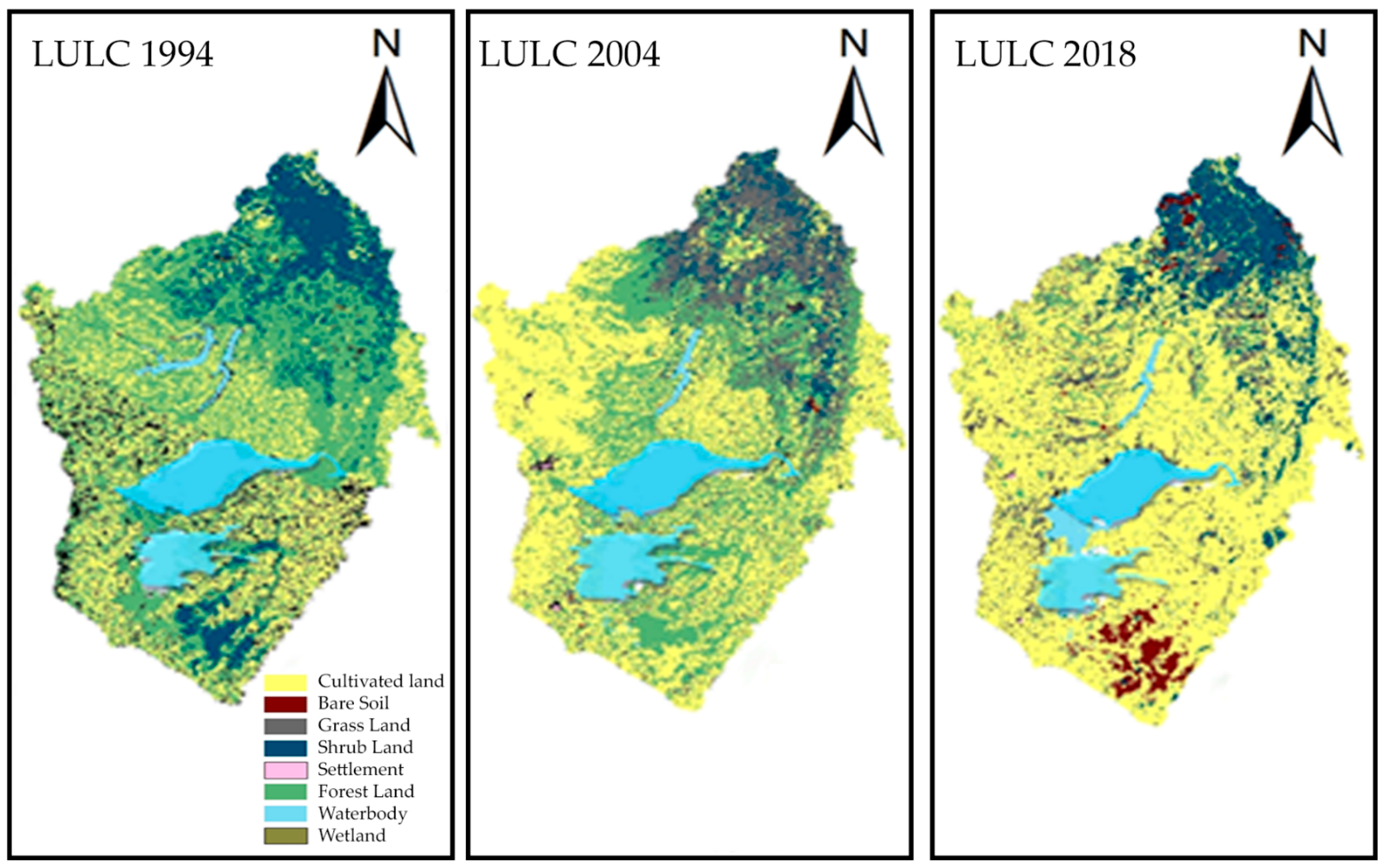
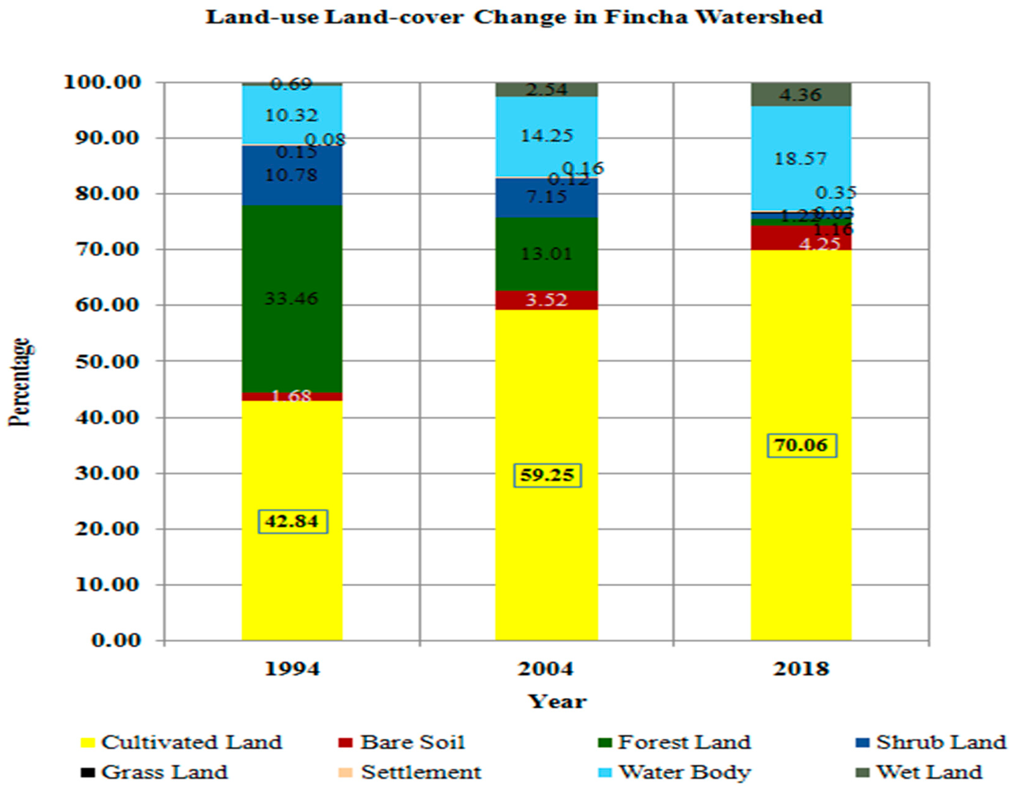
3.1. Land Use Land Cover Changes

Land use land cover changes of the Fincha’a Watershed were observed for three reference years (1994, 2004, and 2018) using Landsat satellite imagery and supervised classification, and compared accounting for eight classes (Table 4). For qualitative comparison, Figure 9 and Figure 10 were created, while the quantitative information is reported in

Table 7. LULC in the Fincha’a watershed in 1994, 2004, and 2018. LULCC between 1994 and 2018.

LULC	1994		2004		2018		2018–1994
	%	Area [ha]	%	Area [ha]	%	Area [ha]	%	Area [ha]
Cultivated Land	42.8	137,352.31	59.3	189,976.87	70.1	224,624.24	+87,271.9	+27.22
Bare Soil	1.7	5376.85	3.5	11,265.78	4.3	13,600.26	+8223.4	+2.57
Forest Land	33.5	107,283.40	13.0	41,714.20	1.2	3719.33	−103,564.1	−32.3
Shrub Land	10.8	34,565.07	7.2	22,925.81	1.2	3910.08	−30,655.0	−9.56
Grass Land	0.2	488.97	0.1	391.18	0.1	97.79	−391.2	−0.12
Settlement	0.1	262.66	0.2	525.32	0.4	1161.86	+899.2	+0.27
Water Body	10.3	33,101.79	14.3	45,707.42	18.6	59,563.98	+26,462.2	+8.25
Wetland	0.7	2217.63	2.5	8163.46	4.4	14,012.86	+11,795.2	+3.67
Total	100	320,648.68	100	320,045.70	100	348,016.75

, pointing out a very relevant change in LULC over the study period.

A rapid increase in the cultivated land class is observable during the study period, as this class occupied 42.8% of the total area in 1994 but 70.1% in 2018. As pointed out in similar studies [18], this is due to population growth and socio-economic factors. The bare soil and settlement also gradually increased from 1.7% (1994) to 4.3% (2018) and 0.1% (1994) to 0.4% (2018), respectively. The increment of bare soil can be explained as the result of erosion and the steep slopes of the Fincha’a watershed, while the need for more room for a growing population is obviously the cause of a major percentage of settlements. The water body and wetland features such as rivers, lakes, and swamps were slightly increased from 10.3% (1994) to 18.6% (2018) and 0.7% (1994) to 4.6% (2018), respectively.

On the contrary, other land use classes decreased over the 25 years study period. For instance, forest land has been greatly decreased from 33.5% in 1994 to only 1.2% in 2018, with a net decline of 32.1%, mostly due to the expansion of agricultural land. Urbanization and agricultural expansion also cause a reduction of the areas covered by shrub and grass, which were degraded by a net percent of 9.6% and 0.1%, respectively.

In 1994, cultivated land and forest land were 42.8% (137,352.31 ha) and 33.5% (107,283 ha), respectively, while shrubland, waterbody, bare soil, wetland, grassland, and settlement area were 10.8% (34,565.07 ha), 10.3% (33,101.79 ha), 1.7% (5376.85 ha), 0.7% (2217.63 ha), 0.2% (488.97 ha), and 0.1% (262.66), respectively. Therefore, in this specific year, cultivated land and forest land were the dominant classes.

In 2004, cultivated land and forest land were 59.3% (189,976.87 ha) and 13.0% (41,714.20 ha), while shrubland, waterbody, bare soil, wetland, grassland, and settlement were 7.2% (22,925.81 ha), 14.3% (45,707.42 ha), 3.5% (11,265.78 ha), 2.5% (8163.46 ha), 0.12% (391.18 ha), and 0.2% (525.32 ha), respectively. Furthermore, throughout the study period, cultivated land has been the most dominant land use class.

In 2018, cultivated land and forest land were respectively 70.1% (224,624.24 ha) and 1.2% (3719.33 ha), while shrubland, waterbody, bare soil, wetland, grassland, and settlement were 1.2% (3910.08 ha), 18.6% (59,563.98 ha), 4.3% (13,600.26 ha), 4.4% (14,012.86 ha), 0.1 (97.79 ha), and 0.4% (1161.86 ha), respectively. The result shows that, in 2018, grassland and forest land were negligible and cultivated land is the most predominant LULC class in the Fincha’a watershed.

The results reported here are in line with the recent work of Tolessa et al. [53], who analysed the Fincha’a watershed LULCC over the period 1987–2019, showing an increment of cultivated areas, settlement, waterbodies, and sugarcane plantation. Such changes involved a significant reduction in areas covered by forest land, wetland, and bare land.

In their work, Dibaba et al. [38] confirmed that anthropogenic activities, such as the construction of the reservoir and the connected river training works, were found to be predominant and immediate as compared to the natural process as a driver of LULCC in the Fincha’a basin. In particular, the hydro-development process affected the local communities and their livelihoods, mostly by changing access to land and reducing the available water [54]. As an example, the seasonal fluctuations of water levels often inundate the croplands of the farmers settled near the water bodies. Furthermore, most of the present land-use practices in the catchment are focused on short-term supply satisfaction, which could involve long-term loss of ecosystem services and damage to the environment.

3.2. Land Use Classification Accuracy

In this study, the random reference points are 178, 249, and 318 for the years 1994, 2004, and 2018, respectively. To assess the classification accuracy, confusion matrixes were derived using the ERDAS Imagine 2014 and GIMP 2.10.12 software. It is worth noting here that the following results depend on the used classification method and the experience of the operator.

Table 8. Confusion matrix of LULC in 1994 (S: Settlement; WL: Water body; SHL: Shrub land; CL: Cultivated land; GL: Grassland; FL: Forest land; BS: Bare soil).

LULC	S	WL	SHL	WB	CL	GL	FL	BS	Total	User (%)
S	8	0	1	0	1	0	2	0	12	66.67
WL	1	18	0	2	0	1	0	1	23	78.26
SHL	0	1	15	0	2	0	0	0	19	78.95
WB	1	0	1	21	0	0	1	0	24	87.50
CL	0	3	0	0	27	1	0	0	31	87.10
GL	0	0	0	0	0	15	3	2	20	75.00
FL	0	2	0	0	0	0	33	1	36	91.67
BS	0	0	0	0	0	2	0	16	20	100.00
Total	10	24	16	23	30	19	36	20	178	OA = 86.06
Producer’s (%)	80.00	75.00	93.75	91.30	90.00	78.95	91.67	80		Ka = 83.61

Overall classification accuracy (OA) = 86.06%; Kappa coefficient (K) = 83.61%.

,

Table 9. Confusion matrix of LULC in 2004 (S: Settlement; WL: Water body; SHL: Shrub land; CL: Cultivated land; GL: Grassland; FL: Forest land; BS: Bare soil).

LULC	S	WL	SHL	WB	CL	GL	FL	BS	Total	User’s (%)
S	10	1	0	1	0	0	1	0	13	76.92
WL	0	35	1	0	2	0	0	0	38	92.11
SHL	1	0	32	0	0	0	0	1	34	94.12
WB	0	0	1	33	0	2	0	0	36	91.67
CL	0	0	0	0	40	0	2	1	43	93.02
GL	0	0	3	0	3	20	0	0	26	76.92
FL	0	1	0	1	0	2	34	0	38	89.47
BS	0	0	0	0	0	3	0	18	21	85.71
Total	11	37	37	35	45	27	37	20	249	OA = 89.16
Producer’s (%)	90.91	94.59	86.49	94.29	88.89	74.07	91.89	90.00		Ka = 87.43

Overall classification accuracy (OA) = 89.16%; Kappa coefficient (K) = 87.43%.

and

Table 10. Confusion matrix of LULC in 2018 (S: Settlement; WL: Water body; SHL: Shrub land; CL: Cultivated land; GL: Grassland; FL: Forest land; BS: Bare soil).

LULC	S	WL	SHL	WB	CL	GL	FL	BS	Total	User’s (%)
S	15	0	0	0	1	2	0	0	18	83.33
WL	0	43	1	0	0	0	1	0	45	95.56
SHL	1	0	40	1	0	1	0	1	44	90.91
WB	0	1	0	41	1	0	0	0	43	95.35
CL	0	0	1	0	48	0	2	1	52	92.31
GL	0	1	0	2	0	30	0	0	33	90.91
FL	1	0	0	0	1	1	42	0	45	93.33
BS	0	1	1	0	0	0	1	35	38	92.11
Total	17	46	43	44	51	34	46	37	318	OA = 92.45
Producer’s (%)	88.24	93.48	93.02	93.18	94.12	88.24	91.30	94.59		Ka = 91.30

Overall classification accuracy (OA) = 92.45%; Kappa coefficient (K) = 91.30%.

show the confusion matrix for the three Landsat images, pointing out that the overall classification accuracy of the total number of correctly classified pixels (diagonal) to the total number of reference pixels was 92.52%, 92.71%, and 94.44% for 1994, 2004, and 2018, respectively. According to Anderson [23], the minimum accuracy value for reliable land cover classification is 85%, therefore the results presented here satisfy the minimum accuracy assessment criteria. The user’s accuracy (error of commission or inclusion) and producers’ (error of omission or exclusion) which are used to evaluate the classification accuracy were also calculated.

Table 8 shows that, for the reference year 1994, the percentage of overall accuracy and kappa coefficient were 86.06% and 83.61%, respectively. The grey-highlighted diagonal number in the matrix indicated correctly classified pixels for each LULC class, with the yellow cell indicating the total number of correctly classified pixels.

Table 9 shows that the classified map of 2004 has an overall accuracy of 89.16% and a kappa coefficient of 87.43%. In this case, it is possible to notice a higher number of pixels correctly classified.

In 2018, the overall accuracy and kappa coefficients were 92.45% and 91.30%, respectively (Table 10), with the highest number of correctly classified pixels during the study period.

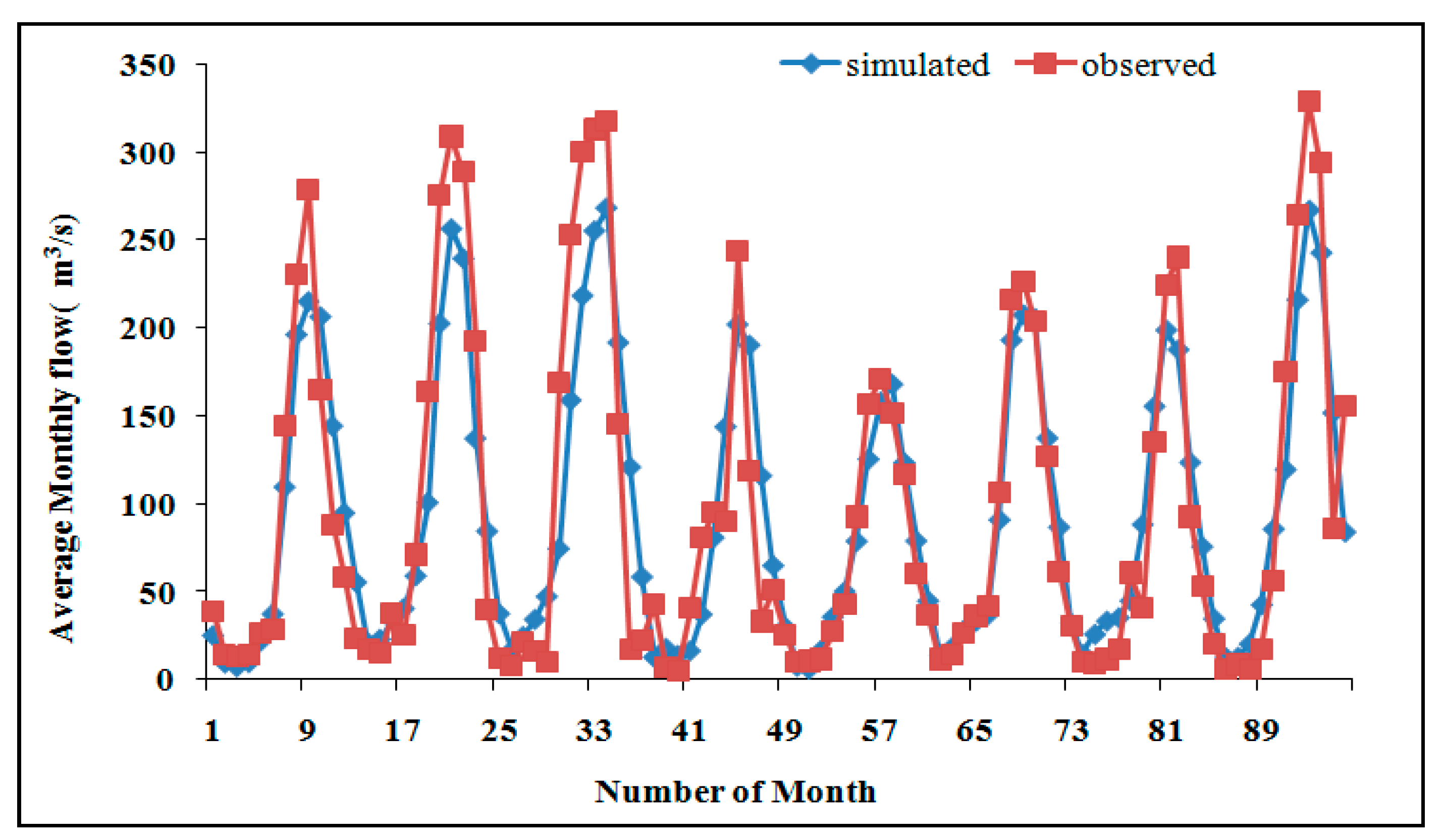
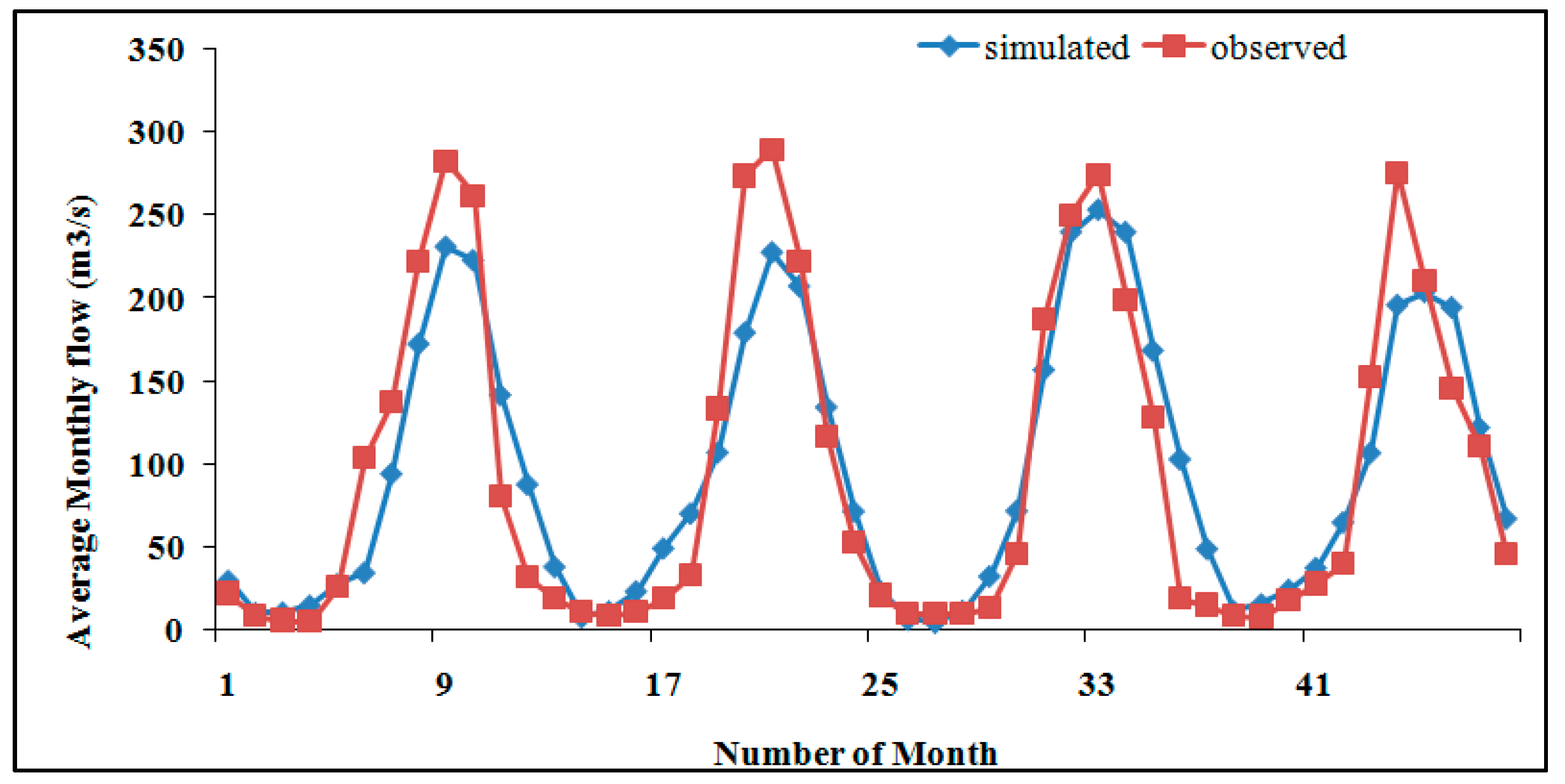
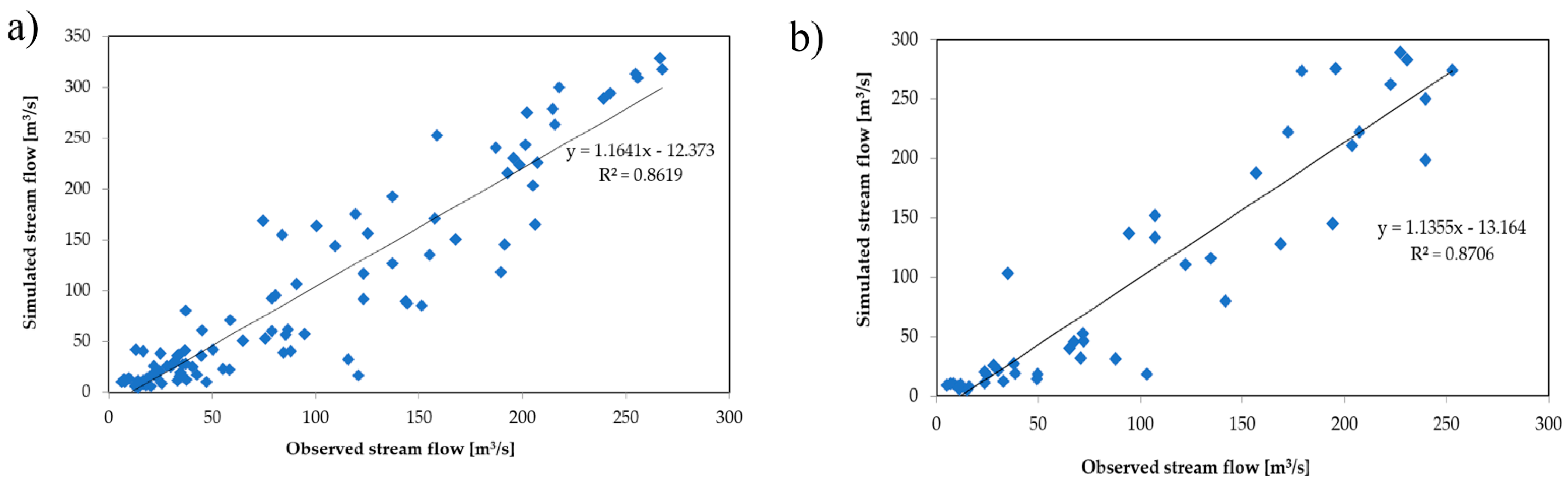
3.3. Calibration and Validation of the Streamflow

The simulated streamflow was calibrated against an observed discharge, considering a period of 8 years (1997–2004) and monthly data. The first 3 years were used as the warm-up period, while the rest were for model calibration. The coefficient of determination and the Nash-Sutcliffe equation (Section 2.4.7) have been used as parameters to determine the quality of the performed calibrations. As visible from Figure 11, the SWAT model is able to reproduce the measured water flow in a rather satisfactory manner (R² = 0.86, NSE = 0.85), with a slight underestimation of the peaks.

The Fincha’a streamflow was validated for 4 years, between 2005 and 2008. As visible in Figure 12, the validation processes provided good results, with a correlation coefficient R² = 0.87 and a Nash-Sutcliffe coefficient NSE = 0.84. Moreover, in this case, it is possible to observe an underestimation of the peak conditions which, however, does not influence the overall simulation.

Table 11. Model performance evaluation statistics.

	R2	NSE	PBIAS
Calibration (1997–2004)	0.86	0.85	+1.13
Validation (2005–2008)	0.87	0.84	−2.806

summarizes the parameters used for evaluating the model performance during the calibration and validation process (Section 2.4.7), while Figure 13 provides a scatter plot of the simulated and observed flow values for the two periods. Based on such results, it can be concluded that the SWAT model can be applied to have a reliable prediction of the streamflow of the Fincha’a watershed.

Based on these results, it is possible to observe that the model proposed here performs better than a similar model developed by Ayana et al. in 2012 [51]. Indeed, they obtained an R² of 0.82 and 0.81 for the calibration (1987–1996) and simulation (1997–2006) periods, respectively. They attributed that the differences between simulated and observed values might be attributed to errors in creating rainfall inputs, but also to the fact that surface water coming from the reservoir used for water supply and irrigation were not included in the simulation. Even if using different periods for calibrating and validating the SWAT model, the present study pointed out similar drawbacks, which are intrinsically connected with the study, due to the lack of information on multiple uses of the water coming from the Fincha’a reservoir.

3.4. Hydrological Response to LULCC Changes on Streamflow

As already observed, the hydrologic responses of watershed processes are generally highly affected by LULCC [52]. Crucial watershed processes that can be affected by LULCC are surface runoff, lateral flow, and groundwater flow.

Table 12. Observed average flow during the dry and wet months.

Period	Average Flow [m3/s]			Change of Flow [m3/s]
	1994	2004	2018	1994–2004	2004–2018	1994–2018
dry months	10.72	15.89	25.86	+5.2	+9.5	+14.6
wet months	132.67	167.85	194.67	+35.2	+26.8	+62.0

shows the stream flow simulated accounting for the LULCC situation in the three reference years, classifying it into wet (August, September, and October) and dry months (February, March, and April).

It is possible to notice that the average dry monthly streamflow increased by 5.17 m³/s between 1994 and 2004, 9.47 m³/s from 2004 to 2018, and 14.64 m³/s over the whole period (1994–2018). This means that, during the 25 years, the dry-months discharge increased by 8.3%. The average wet month flow was more influenced by LULCC, increasing by 35.18, 26.82, and 62 m³/s between 1994–2004, 2004–2018, and 1994–2018, respectively.

This analysis can reveal that the increment of cultivated land causes a direct increase in surface runoff, mostly during the wettest months. Changes in the areas covered by wetland and water bodies also cause a slight increase in flow discharge during the driest months.

3.5. Sensitivity Analysis

As anticipated in Section 2.4.5, the sensitivity analysis pointed out that, out of 26 possible parameters, only twelve have a relevant influence in controlling the hydrological processes in the watershed (

Table 13. Streamflow sensitivity parameters.

S. No.	Parameter	Definition	Fitted Value	Max_Value	Min_Value
1	SOL_K	Saturated Hydraulic conductivity	0.24	−0.8	0.8
2	ALPHA_BF	Base flow alpha factor (days)	0.85	0	1
3	GW_DELAY	Ground water delay (days)	51	30	450
4	GWQMN	The threshold depth of water shallow aquifer	0.3	0	2
5	GW_REVAP	Groundwater revamp coefficient	0.11	0	0.2
6	ESCO	Soil evaporation compensation factor	0.93	0.8	1
7	CH_N2	Manning’s roughness coefficient	0.045	0	0.3
8	CH_K2	Effective hydraulic conductivity	23.75	5	130
9	ALPHA_BNK	Baseflow alpha factor for bank storage	0.45	0	1
10	SOL_AWC	Soil available water capacity	−0.17	−0.2	0.4
11	CN2	SCS runoff Curve number for moisture condition II	−0.18	−0.2	0.2
12	SOL_BD	Moist bulk density	0.105	−0.5	0.6

). Based on a previous work of Leta et al. [33], saturated hydraulic conductivity, base flow alpha factor, groundwater delay, and the depth of the water aquifer were considered the most important sensitive parameters to be used in the calibration process.

3.6. Recommendations

Based on the present study, some recommendations can be provided.

• No gauging stations are yet installed in the lower part of the Fincha’a watershed, while some of them are installed in the upper part. For the future, greater efforts are needed to install stations evenly distributed in the watershed, aiming to obtain a better monitoring network, which can be used for inferring basin-wide information on the hydro-meteorological dynamics.
• At this moment, there is a reduced agreement on the watershed delineation. In fact, for defining the basin borders, some researchers used the outlet of the Chomen Lake, while others prefer the right bank of the Abbay River. This can result in dissimilarities and uncertainties between the results of studies such as the one presented here, and foster a debate among researchers. To solve the situation, the Abbay Basin Authority office should give a clear description of watershed delineation, support decisions, and update information by re-organizing the management information system.
• To develop more accurate hydrological models such as the one shown here, improved monitoring devices and protocols are needed. Indeed, the present gauging network does not allow for developing a precise and basin-wide water use budget, knowing, for example, how much water of the reservoir is used for domestic uses or irrigation.
• The great expansion of cultivated land exposes the local community to cutting trees for fuel, construction of timber, and generation of additional income, but negatively affects the natural environment. However, it could be better to wisely use the natural resources, managing them in an integrated, participatory, equitable, and sustainable manner.
• For the future, there is the need of integrating similar studies of LULCC with research looking at the effect of LULCC on the natural capital (see, for example, [53]), for public awareness and decision-making processes at the watershed level for sustainable development.
• If the past trends in LULCC will persist in the future, the observed increase in surface runoff and peak events, as well as soil erosion, could be eventually fostered by climate change, with unforeseen consequences on the environment [54] and the local livelihood [55,56]. Therefore, there is the need for further research, accounting for not only the most up-to-date climate scenarios but also the interrelationship between the natural and the built environment.
• Differently from anthropogenic drivers, natural variations such as climate change affect the environment and the connected ecosystem services at a longer time scale [36,37,38], and therefore future studies should consider longer horizons to effectively account for the combined effects of both natural and human-induced alterations.

4. Conclusions

This study developed a SWAT model to investigate the hydrological responses to LULCC in the Ethiopian Fincha’a watershed. To do this, multiple steps were followed. Firstly, satellite images were used to produce LULCC maps for three reference years, chosen within a period of 25 years (1994–2018). Once determined, the most significant classes covering the whole basin, weather, and hydrological data, combined with a topographical base derived from a rather coarse DEM, were used to infer information on the surface runoff over the entire watershed, needed for model calibration and validation.

Comparing the LULCC derived from satellite images, it is possible to observe a significant decline of forest land (−32.3%) and shrubland (−9.6%) between 1994 and 2018, mostly due to the creation of new agricultural zones (+27.2%) and settlement (+3.7%) to answer to an increasing population that needs new means of subsistence. The quality of the supervised classification used for deriving LULCC maps was checked via confusion matrixes, showing an overall accuracy of 86.1%, 89.2%, and 92.5% and corresponding kappa coefficients of 83.6%, 87.4%, and 91.3%, for the reference years 1994, 2004, and 2018, respectively

The overall efficiency of the SWAT model was evaluated by the coefficient of determination and the Nash-Sutcliffe parameters, which resulted higher than 0.84 for both the calibration and validation periods, indicating that the model provided reliable outcomes. Once calibrated and validated, the model was applied and the outcomes pointed out that the LULCC observed in the Fincha’a basin caused an increase in surface runoff, more prominent during the wet months (August–October).

As similar research performed across Ethiopia have pointed out [see review 18], this study provides important insights on the basin-wide effects of LULCC on the Fincha’a catchment hydrology, to be used by decision-makers for planning future management strategies to assure a suitable future of the Fincha’a watershed.

References

- Abbott, M.B.; Refsgaard, J.C. (Eds.) Distributed Hydrological Modelling; Springer Science & Business Media: Dordrecht, The Netherlands, 2012; Volume 22. [Google Scholar]
- Butchart, S.; Walpole, M.; Collen, B.; Van Strien, A.; Scharlemann, J.; Almond, R.; Baillie, J.E.; Bomhard, B.; Brown, C.; Bruno, J.; et al. Global biodiversity: Indicators of recent declines. Science 2010, 328, 1164–1168. [Google Scholar] [CrossRef]
- Githui, F.; Mutua, F.; Bauwens, W. Estimating the impacts of land cover change on runoff using the soil and water assessment tool (SWAT): Case study of Nzoia catchment, Kenya. Hydrol. Sci. J. 2010, 54, 899–908. [Google Scholar] [CrossRef]
- Kennedy, R.E.; Yang, Z.; Braaten, J.; Copass, C.; Antonova, N.; Jordan, C.; Nelson, P. Attribution of disturbance change agent from Landsat time-series in support of habitat monitoring in the Puget Sound region, USA. Remote Sens. Environ. 2015, 166, 271–285. [Google Scholar] [CrossRef]
- Li, M.S.; Mao, L.J.; Shen, W.J.; Liu, S.Q.; Wei, A.S. Change and fragmentation trends of Zhanjiang mangrove forests in southern China using multi-temporal Landsat imagery (1977–2010). Estuar. Coast. Shelf Sci. 2013, 130, 111–120. [Google Scholar] [CrossRef]
- Kamwi, J.; Cho, M.; Kaetsch, C.; Manda, S.; Graz, F.; Chirwa, P. Assessing the Spatial Drivers of Land Use and Land Cover Change in the Protected and Communal Areas of the Zambezi Region, Namibia. Land 2018, 7, 131. [Google Scholar] [CrossRef] [Green Version]
- Vermote, E.; Justice, C.; Claverie, M.; Franch, B. Preliminary analysis of the performance of the Landsat 8/OLI land surface reflectance product. Remote Sens. Environ. 2016, 185, 46–56. [Google Scholar] [CrossRef]
- Souza-Filho, P.W.M.; de Souza, E.B.; Silva Júnior, R.O.; Nascimento, W.R., Jr.; de Mendonça, B.R.V.; Guimarães, J.T.F.; Dall’Agnol, R.; Siqueira, J.O. Four decades of land-cover, land-use and hydroclimatology changes in the Itacaiúnas River watershed, southeastern Amazon. J. Environ. Manag. 2016, 167, 175–184. [Google Scholar] [CrossRef] [PubMed]
- Shen, G.; Ibrahim, A.N.; Wang, Z.; Ma, C.; Gong, J. Spatial—Temporal land-use/land-cover dynamics and their impacts on surface temperature in Chongming Island of Shanghai, China. Int. J. Remote Sens. 2015, 36, 4037–4053. [Google Scholar] [CrossRef]
- Park, J.K.; Um, D.Y. Time series analysis of land cover and land surface temperature change using remote sensing method in Seoul. Int. J. Appl. Eng. Res. 2015, 10, 39201–39207. [Google Scholar]
- Dissanayake, S.; Asafu-Adjaye, J.; Mahadeva, R. Addressing climate change cause and effect on land cover and land use in South Asia. Land Use Policy 2017, 67, 352–366. [Google Scholar] [CrossRef]
- Calder, C. Hydrologic effects of land use change. In Handbook of Hydrology; Maidment, D.R., Ed.; McGraw-Hill: New York, NY, USA, 1993. [Google Scholar]
- Garg, V.; Nikam, B.R.; Thakur, P.K.; Aggarwal, S.P.; Gupta, P.K.; Srivastav, S.K. Human-induced land use land cover change and its impact on hydrology. HydroResearch 2019, 1, 48–56. [Google Scholar] [CrossRef]
- Alam, A.; Bhat, M.S.; Maheen, M. Using Landsat satellite data for assessing the land use and land cover change in Kashmir valley. GeoJournal 2020, 85, 1529–1543. [Google Scholar] [CrossRef] [Green Version]
- Leta, M.K.; Demissie, T.A.; Tränckner, J. Modeling and Prediction of Land Use Land Cover Change Dynamics Based on Land Change Modeler (LCM) in Nashe Watershed, Upper Blue Nile Basin, Ethiopia. Sustainability 2021, 13, 3740. [Google Scholar] [CrossRef]
- Zoungrana, B.J.; Conrad, C.; Amekudzi, L.K.; Thiel, M.; Da, E.D.; Forkuor, G.; Löw, F. Multi-temporal landsat images and ancillary data for land use/cover change (LULCC) detection in the Southwest of Burkina Faso, West Africa. Remote Sens. 2015, 7, 12076–12102. [Google Scholar] [CrossRef] [Green Version]
- Di Gregorio, A.D.; Jansen, L.J. Land Cover Classification System, Classification Concepts and User Manual, Software version 2; Food and Agriculture Organization of the United Nations: Rome, Italy, 2005. [Google Scholar]
- Regasa, M.S.; Nones, M.; Adeba, D. A Review on Land Use and Land Cover Change in Ethiopian Basins. Land 2021, 10, 585. [Google Scholar] [CrossRef]
- Desta, H.; Fetene, A. Land-use and land-cover change in Lake Ziway watershed of the Ethiopian Central Rift Valley Region and its environmental impacts. Land Use Policy 2020, 96, 104682. [Google Scholar] [CrossRef]
- Dwivedi, R.S.; Sreenivas, K.; Ramana, K.V. Cover: Land-use/land-cover change analysis in part of Ethiopia using Landsat Thematic Mapper data. Int. J. Remote. Sens. 2005, 26, 1285–1287. [Google Scholar] [CrossRef]
- Meyer, W.B.; Turner, B.L., II. Change in Land Use and Land Cover: A Global Perspective; Cambridge University Press: Cambridge, MA, USA, 1994; 537p. [Google Scholar]
- Lambin, E.F.; Turner, B.L.; Geist, H.J.; Agbola, S.B.; Angelsen, A.; Bruce, J.W.; Coomes, O.T.; Dirzog, R.; Fischerh, G.; Folke, C.; et al. The causes of land-use and land-cover change: Moving beyond the myths. Glob. Environ. Chang. 2001, 11, 261–269. [Google Scholar] [CrossRef]
- Anderson, J.H. A Land Use and Land Cover Classification System for Use with Remote Sensor Data; Geological Survey Professional Paper; US Government Printing Office: Washington, DC, USA, 1976; Volume 964. [Google Scholar]
- Zhang, L.; Nan, Z.; Yu, W.; Ge, Y. Hydrological responses to land-use change scenarios under constant and changed climatic conditions. Environ. Manag. 2016, 57, 412–431. [Google Scholar] [CrossRef]
- Cüceloğlu, G.; Seker, D.Z.; Tanik, A.; Öztürk, İ. Analyzing Effects of Two Different Land Use Datasets on Hydrological Simulations by Using SWAT Model. Int. J. Environ. Geoinform. 2021, 8, 172–185. [Google Scholar] [CrossRef]
- Polanco, E.I.; Fleifle, A.; Ludwig, R.; Disse, M. Improving SWAT model performance in the upper Blue Nile Basin using meteorological data integration and subcatchment discretization. Hydrol. Earth Syst. Sci. 2017, 21, 4907–4926. [Google Scholar] [CrossRef] [Green Version]
- de Serrão, E.A.O.; Silva, M.T.; Ferreira, T.R.; de Ataide, L.C.P.; dos Santos, C.A.; de Lima, A.M.M.; Gomes, D.J.C. Impacts of land use and land cover changes on hydrological processes and sediment yield determined using the SWAT model. Int. J. Sediment Res. 2021, in press. [Google Scholar]
- Markhi, A.; Laftouhi, N.; Grusson, Y.; Soulaimani, A. Assessment of potential soil erosion and sediment yield in the semi-arid N′ fis basin (High Atlas, Morocco) using the SWAT model. Acta Geophys. 2019, 67, 263–272. [Google Scholar] [CrossRef]
- Negese, A. Impacts of Land Use and Land Cover Change on Soil Erosion and Hydrological Responses in Ethiopia. Appl. Environ. Soil Sci. 2021, in press. [Google Scholar] [CrossRef]
- Worku, T.; Khare, D.; Tripathi, S.K. Modeling runoff–sediment response to land use/land cover changes using integrated GIS and SWAT model in the Beressa watershed. Environ. Earth Sci. 2017, 76, 1–14. [Google Scholar] [CrossRef]
- Ethiopian Water Resources Management Policy. 1999. Available online: http://www.fao.org/faolex/results/details/en/c/LEX-FAOC158196 (accessed on 1 April 2021).
- Moriasi, D.N.; Arnold, J.G.; Van Liew, M.W.; Bingner, R.L.; Harmel, R.D.; Veith, T.L. Model evaluation guidelines for systematic quantification of accuracy in watershed simulations. Trans. ASABE 2007, 50, 885–900. [Google Scholar] [CrossRef]
- Leta, M.K.; Demissie, T.A.; Koriche, S.A. Impacts of Land Use Land Cover Change on Sediment Yield and Stream Flow: A Case of Finchaa Hydropower Reservoir, Ethiopia. Int. J. Sci. Technol. 2017, 6, 763–781. [Google Scholar]
- Berihun, M.L.; Tsunekawa, A.; Haregeweyn, N.; Meshesha, D.T.; Adgo, E.; Tsubo, M.; Masunaga, T.; Fenta, A.A.; Sultan, D.; Yibeltal, M.; et al. Hydrological responses to land use/land cover change and climate variability in contrasting agro-ecological environments of the Upper Blue Nile basin, Ethiopia. Sci. Total. Environ. 2019, 689, 347–365. [Google Scholar] [CrossRef]
- Warburton, M.L.; Schulze, R.E.; Jewitt, G.P. Hydrological impacts of land use change in three diverse South African catchments. J. Hydrol. 2012, 414, 118–135. [Google Scholar] [CrossRef]
- Tessema, I.; Simane, B. Vulnerability analysis of smallholder farmers to climate variability and change: An agro-ecological system-based approach in the Fincha’a sub-basin of the upper Blue Nile Basin of Ethiopia. Ecol. Process. 2019, 8, 1–18. [Google Scholar] [CrossRef] [Green Version]
- Tefera, B.; Sterk, G. Hydropower-induced land use change in Fincha’a watershed, western Ethiopia: Analysis and impacts. Mt. Res. Dev. 2008, 28, 72–80. [Google Scholar] [CrossRef] [Green Version]
- Dibaba, W.T.; Demissie, T.A.; Miegel, K. Drivers and implications of land use/land cover dynamics in Finchaa catchment, northwestern Ethiopia. Land 2020, 9, 113. [Google Scholar] [CrossRef] [Green Version]
- Prabhadevi, Y.G.K.L.; Sreenivasa, V.; Mengistou, S. A Study on Phytoplankton Species Composition, and Primary Production in Fincha Reservoir, West Shoa Zone, Ethiopia. J. Nat. Sci. Res. 2015, 5, 23–30. [Google Scholar]
- Bezuayehu, T. People and dams: Environmental and socio-economic impact Fincha’a Hydropower dam, western Ethiopia. Trop. Res. Manag. Papers 2006, 75, Wageningen University, Wageningen, the Netherlands. [Google Scholar]
- Makin, M.K. Prospects for Irrigation Development around Lake Ziway, Ethiopia. Land Resour. Study Div. 1976, 26, 1–132. [Google Scholar]
- Natural Resources Conservation Service; Agriculture Department (Eds.) Keys to Soil Taxonomy; Government Printing Office: Washington, DC, USA, 2010. [Google Scholar]
- Gyanesh, C.; Brian, L.M.; Dennis, L.H. Summary of current radiometric calibration coefficients for Landsat MSS, TM, ETM+, and EO–1 ALI sensors. Remote. Sens. Environ. 2009, 113, 893–903. [Google Scholar]
- Tamiru, H.; Wagari, M. Comparison of ANN model and GIS tools for Delineation of Groundwater Potential Zones, Fincha Catchment, Abay Basin, Ethiopia. Geocarto Int. 2021, 1–13, accepted. [Google Scholar] [CrossRef]
- Taye, H. Dynamics of Land Use Land Cover Changes on Stream Flow in Fincha Amerti Neshe Sub-Basin. Master’s Thesis, School of Graduate Studies of Addis Abeba University, Addis Abeba, Ethiopia, 2016. [Google Scholar]
- Campbell, W.G.; Mortenson, D.C. Ensuring the quality of geographic information System data: A practical application of quality control. Photogramm. Eng. Remote. Sens. 1989, 55, 1613–1618. [Google Scholar]
- Setegn, S.G.; Srinivasan, R.; Dargahi, B.; Melesse, A.M. Spatial delineation of soil erosion vulnerability in the Lake Tana Basin, Ethiopia. Hydrol. Process. Int. J. 2009, 23, 3738–3750. [Google Scholar] [CrossRef]
- Danuso, F. A Stochastic Model for weather data generation. Ital. J. Agron. 2002, 6, 57–72. [Google Scholar]
- Arnold, J.G.; Srinivasan, R.; Muttiah, R.R.; Williams, J.R. Large Area Hydrologic Modeling and Assessment Part I: Model Develop. J. Am. Water Resour. Assoc. 1998, 34, 73–89. [Google Scholar] [CrossRef]
- Ayana, A.B.; Edossa, D.C.; Kositsakulchai, E. Simulation of sediment yield using SWAT model in Fincha Watershed, Ethiopia. Agric. Nat. Resour. 2012, 46, 283–297. [Google Scholar]
- Da Silva, M.G.; de Aguiar Netto, A.D.O.; de Jesus Neves, R.J.; Do Vasco, A.N.; Almeida, C.; Faccioli, G.G. Sensitivity analysis and calibration of hydrological modeling of the watershed Northeast Brazil. J. Environ. Prot. 2015, 6, 837. [Google Scholar] [CrossRef] [Green Version]
- Tolessa, T.; Kidane, M.; Bezie, A. Assessment of the linkages between ecosystem service provision and land use/land cover change in Fincha watershed, North-Western Ethiopia. Heliyon 2021, 7, e07673. [Google Scholar] [CrossRef]
- Müller-Mahn, D.; Gebreyes, M. Controversial connections: The water-energy-food nexus in the Blue Nile basin of Ethiopia. Land 2019, 8, 135. [Google Scholar] [CrossRef] [Green Version]
- Kumar, S.; Mishra, A. Critical erosion area identification based on hydrological response unit level for effective sedimentation control in a river basin. Water Resour. Manag. 2015, 29, 1749–1765. [Google Scholar] [CrossRef]
- Chimdessa, K.; Quraishi, S.; Kebede, A.; Alamirew, T. Effect of land use land cover and climate change on river flow and soil loss in Didessa River Basin, South West Blue Nile, Ethiopia. Hydrology 2019, 6, 2. [Google Scholar] [CrossRef] [Green Version]
- Dibaba, W.T.; Demissie, T.A.; Miegel, K. Prioritization of Sub-Watersheds to Sediment Yield and Evaluation of Best Management Practices in Highland Ethiopia, Finchaa Catchment. Land 2021, 10, 650. [Google Scholar] [CrossRef]