Article

Quantifying Drivers of Coastal Forest Carbon Decline Highlights Opportunities for Targeted Human Interventions

1
Center for Geospatial Analytics, College of Natural Resources, North Carolina State University, 2800 Faucette Drive, Raleigh, NC 27695, USA
2
Department of Parks, Recreation, and Tourism Management, College of Natural Resources, North Carolina State University, 2800 Faucette Drive, Raleigh, NC 27695, USA
3
Department of Wildlife Ecology and Conservation, University of Florida, Gainesville, FL 32611, USA
4
AidData Global Research Institute, The College of William and Mary, 424 Scotland Street, Williamsburg, VA 23185, USA
5
Center for Geospatial Analysis, The College of William and Mary, 400 Landrum Dr., Williamsburg, VA 23185, USA
6
Department of Environment and Society, Utah State University, Logan, UT 84322, USA
*
Author to whom correspondence should be addressed.
Land 2021, 10(7), 752; https://doi.org/10.3390/land10070752
Submission received: 18 June 2021 / Revised: 14 July 2021 / Accepted: 14 July 2021 / Published: 18 July 2021
(This article belongs to the Special Issue Land Modifications and Impacts on Coastal Areas)

Abstract

:
As coastal land use intensifies and sea levels rise, the fate of coastal forests becomes increasingly uncertain. Synergistic anthropogenic and natural pressures affect the extent and function of coastal forests, threatening valuable ecosystem services such as carbon sequestration and storage. Quantifying the drivers of coastal forest degradation is requisite to effective and targeted adaptation and management. However, disentangling the drivers and their relative contributions at a landscape scale is difficult, due to spatial dependencies and nonstationarity in the socio-spatial processes causing degradation. We used nonspatial and spatial regression approaches to quantify the relative contributions of sea level rise, natural disturbances, and land use activities on coastal forest degradation, as measured by decadal aboveground carbon declines. We measured aboveground carbon declines using time-series analysis of satellite and light detection and ranging (LiDAR) imagery between 2001 and 2014 in a low-lying coastal region experiencing synergistic natural and anthropogenic pressures. We used nonspatial (ordinary least squares regression–OLS) and spatial (geographically weighted regression–GWR) models to quantify relationships between drivers and aboveground carbon declines. Using locally specific parameter estimates from GWR, we predicted potential future carbon declines under sea level rise inundation scenarios. From both the spatial and nonspatial regression models, we found that land use activities and natural disturbances had the highest measures of relative importance (together representing 94% of the model’s explanatory power), explaining more variation in carbon declines than sea level rise metrics such as salinity and distance to the estuarine shoreline. However, through the spatial regression approach, we found spatial heterogeneity in the relative contributions to carbon declines, with sea level rise metrics contributing more to carbon declines closer to the shore. Overlaying our aboveground carbon maps with sea level rise inundation models we found associated losses in total aboveground carbon, measured in teragrams of carbon (TgC), ranged from 2.9 ± 0.1 TgC (for a 0.3 m rise in sea level) to 8.6 ± 0.3 TgC (1.8 m rise). Our predictions indicated that on the remaining non-inundated landscape, potential carbon declines increased from 29% to 32% between a 0.3 and 1.8 m rise in sea level. By accounting for spatial nonstationarity in our drivers, we provide information on site-specific relationships at a regional scale, allowing for more targeted management planning and intervention. Accordingly, our regional-scale assessment can inform policy, planning, and adaptation solutions for more effective and targeted management of valuable coastal forests.

1. Introduction

Coastal forests cover less than 3% of the Earth’s surface yet sequester and store as much carbon (C) as their terrestrial counterparts [1,2]. By storing carbon in vegetation and sediments, coastal forests play important roles in biogeochemical carbon (C) cycling and mitigating climate change [3,4]. Coastal forests provide a suite of additional ecosystem services, including storm surge protection, wildlife habitat, water filtration, and recreational opportunities [3,5]. At the terrestrial–ocean interface, coastal forests are disproportionately impacted by pressures from human land use modifications and sea level rise, altering the structure and function of these valuable ecosystems [6]. Sea level rise rates are accelerating, outpacing the average 20th century rates, and leading to increased flooding and erosion, saltwater intrusion, and coastal forest loss [7]. At the same time, rapid population growth, demand for food and fiber, and unconstrained coastal development have caused rapid declines in the health and extent of coastal forests [4]. The interactive effects of sea level rise, land use, and other disturbances (e.g., wildfires) impact the quantity and quality of ecosystem services supplied by coastal forests [8], but regional assessments that account for these effects together are limited [9], and few account for spatial dependencies and nonstationarity in the socio-spatial processes driving ecosystem change. Declines in coastal forest health highlight the need for targeted human interventions. More comprehensive regional assessments that explicitly account for socio-spatial processes are critical to understand how and where different adaptation and management strategies will be most effective.
The exposure of freshwater-dependent coastal forests to saltwater from accelerating rates of sea level rise alters freshwater and terrestrial biota and biogeochemical cycling, subsequently altering the carbon storage potential of coastal forests [10,11,12]. Coastal forests generally share characteristics of both wetlands and uplands, and thus sequester and store carbon in both aboveground biomass (e.g., vegetation) and in hydric soils that provide significant long-term stores of carbon [13]. Though C burial rates are highly variable, global rates for tropical mangrove forests, for example, are approximately 31–34 TgC y−1 compared to 78 TgC y−1 in tropical upland forests, despite covering less than 1% of the area covered by tropical forests [13]. These soils are often peat, water-saturated soils that make conditions favorable for anaerobic decomposition and subsequent carbon storage [11]. Wetland drainage and disturbances such as storm surge inundation can cause the rapid collapse of freshwater peats, particularly after vegetation dies off [14]. However, these dynamics and the associated impacts on carbon storage remain poorly understood. The large C stocks stored in coastal forests’ vegetation and soils highlight the important, yet largely unexamined, role in the global sequestration and storage of carbon that would otherwise remain as atmospheric CO2 and exacerbate climate change [13,15,16,17].
As sea levels rise and storm surge events increase in frequency and severity, saltwater intrusion, the inland movement of seawater via natural and manmade conduits (e.g., streams and irrigation canals), will become increasingly commonplace. Though freshwater-dependent forests can withstand brief periods of inundation and associated saltwater exposure, prolonged periods result in tree mortality and limited regeneration [18,19,20]. More salt-tolerant herbaceous species move into these areas, altering species composition and ecological function [21,22]. The process is often referred to as marsh migration, and the stands of dead or dying trees that remain are known as ‘ghost forests’, marking the landward reach of sea level rise impacts [23]. Along the North American Atlantic and Gulf Coasts, this phenomenon is particularly prevalent because sea level rise rates here are three times the global average of ~0.6 mm yr−1 [24], due in part to rapid land subsidence [25,26]. Coastal forests will continue to retreat landward, provided barriers such as roads, other infrastructure, or incompatible land uses do not exist [6]. Targeted adaptation and management activities can enhance forest resilience or facilitate marsh migration, but this requires knowledge of the environmental and land use conditions affecting site suitability and disturbance regimes.
While coastal forests are particularly vulnerable to sea level rise long term, land use activities, resource management (e.g., water use) and other disturbances (e.g., wildfires) are near-term threats. Land use change, and the interactive effects between land use change and sea level rise, will largely determine where and how much carbon is stored in coastal forests [27]. Land ownership in coastal landscapes involves private landowners and operators as well as local, regional, state, and federal agencies [23,28]. The land use decisions of individuals and organizations have regional impacts and necessitate approaches that account for socio-spatial processes in coastal planning, adaptation, and management. These processes often give rise to spatial heterogeneity in the relationships between environmental, land use, and disturbance drivers and coastal forest change. For example, if the relationship between coastal forest health and canal density changes across the study area, we might infer that the relationship exhibits spatial nonstationarity and that there are unmeasured social processes driving these variations. To understand where and when specific planning and management activities will be most successful, it is critical to not only quantify the relationships between coastal forest change and associated drivers of change [29] but also evaluate how these relationships might vary across space.
To date, research on carbon flux (e.g., the driving processes and controls of C dynamics) in temperate coastal forests has focused on findings from field studies [2,4,30]. These studies are requisite to an understanding of the fine scale processes driving coastal forest carbon change, but their applicability at regional scales is limited. They can be used, however, in conjunction with other data to scale up C cycling estimates for regional and landscape scale assessments. The use of remote sensing data in aboveground carbon estimation, with its broad coverage and moderate-to-high spectral, spatial, and temporal resolutions has become an important field of research in recent years [31]. Carbon has been successfully estimated using derived spectral metrics from multispectral satellite imagery [32,33,34], structural metrics from light detection and ranging (LiDAR) data [35,36,37,38], or a combination of the two [39,40,41] in correlative models linking these metrics with field data and has become a common source for carbon estimation at regional scales. Access to multitemporal remote sensing data provides additional opportunities to measure change in carbon stocks over time; however regional analyses assessing carbon dynamics have focused on upland forests (e.g., [42,43,44,45]), herbaceous marsh (e.g., [46]), and mangrove forests (e.g., [47,48]) and not temperate coastal forests (however, see [49]). These studies also do not quantify the combined effects of the natural and anthropogenic factors driving carbon variability and change at regional scales, nor do they account for the spatial heterogeneity in the strength of the relationships between drivers and aboveground carbon stocks by implementing appropriate spatial modeling approaches. Traditional nonspatial regression models cannot capture local variation (in geographic space) in relationships between drivers and responses (referred to as spatial non-stationarity) [50]. Local spatial regression methods, however, can account for variation resulting from the location (non-stationarity) or the spatial scale considered (grain size, sampling interval, or spatial extent) and are well suited to quantify the relationships between drivers of carbon change and the change itself [51]. All of these are requisite to cost effective adaptation, conservation, and management [13,52].
To address these knowledge gaps, we quantified spatiotemporal patterns of aboveground carbon change over a decade (2001–2014) across one of the largest, most vulnerable regions of coastal forest in North America using a combination of field measurements, multispectral satellite imagery, and LiDAR data. We developed a suite of sea level rise, land use, and disturbance drivers and applied global and local spatial regression approaches to model relationships between these drivers and aboveground carbon change. We address the following questions: (1) How do the relationships between aboveground carbon decline and sea level rise, land use, and natural disturbance drivers vary across the landscape? (2) What are the relative contributions of land use, natural disturbance, and sea level rise drivers to carbon decline? (3) Using the spatial regression models developed, what are the future potential aboveground carbon declines as sea levels rise? Our results strengthen the case for the value of coastal forests’ role in the global carbon cycle and highlight the need for similar research on other carbon pools in coastal forests (e.g., soils). Additionally, understanding the drivers of variability in coastal forests’ carbon stores can help managers allocate resources effectively and implement appropriate conservation, adaptation, and management strategies with the potential to address regional carbon management and climate mitigation needs.

2. Materials and Methods
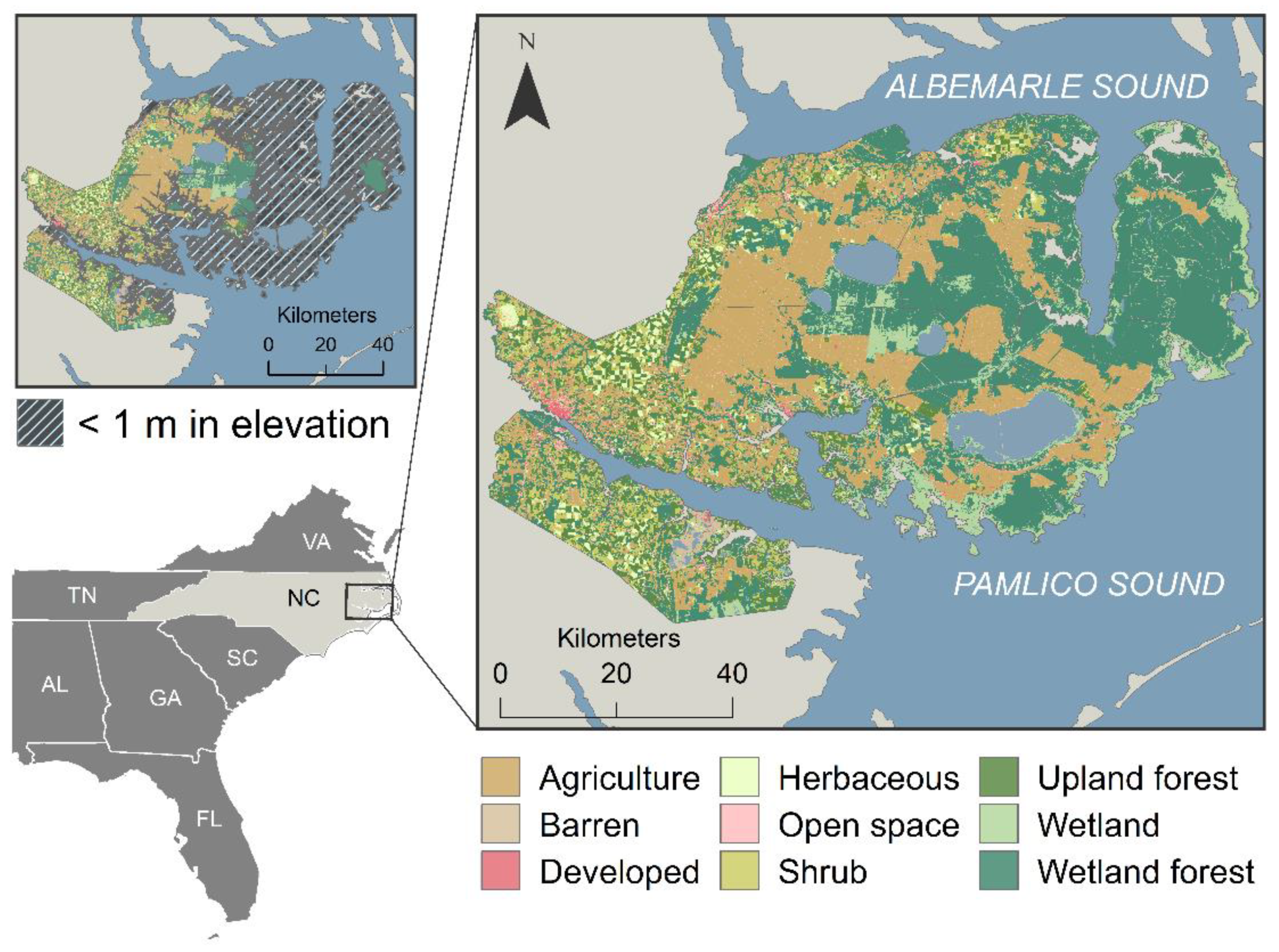
2.1. Study System

The study area is a 4000 km2 coastal region located west of the Albemarle-Pamlico Estuary in Eastern North Carolina and buffered from the Atlantic Ocean by a chain of barrier islands (Figure 1). Forested and herbaceous wetlands, together, cover more than 50 percent of the Albemarle-Pamlico Peninsula. Almost half (47%) of the study area lies below 1 m in elevation, making it particularly vulnerable to sea level rise impacts. Forty percent of the peninsula is publicly owned, most of which can be considered ‘public-non extractive’ land or areas without extractive activities but that may still be managed for biodiversity (e.g., mimicking disturbance events through prescribed fires). ‘Public extractive’ lands are those lands subject to extractive uses (e.g., logging or mining). Private property (60% of the study area) is a mix of natural forest, agricultural lands, and forestry uses. Agriculture and forestry are two main economic drivers, contributing to the state approximately $367 million in agriculture cash receipts and $342.8 million from forest output per year [53]. Industrial forests and agricultural lands occur in low-elevation areas and are thus highly managed with canals, water control structures, and impoundments.

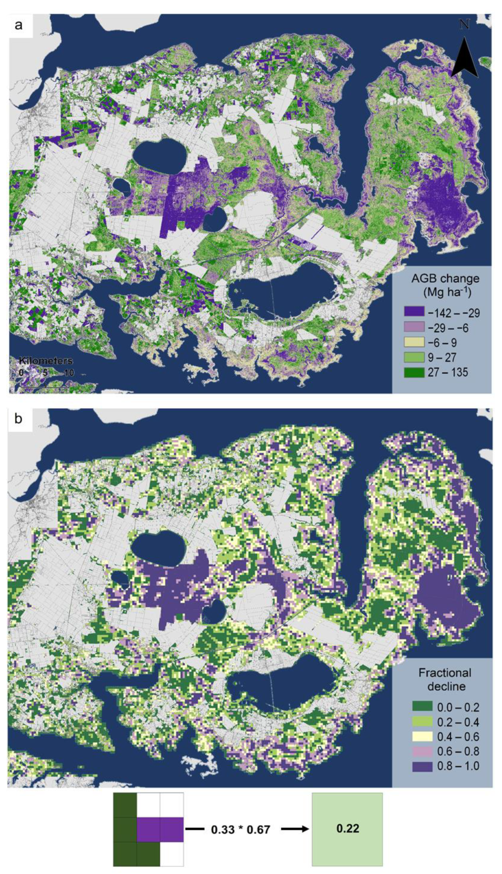
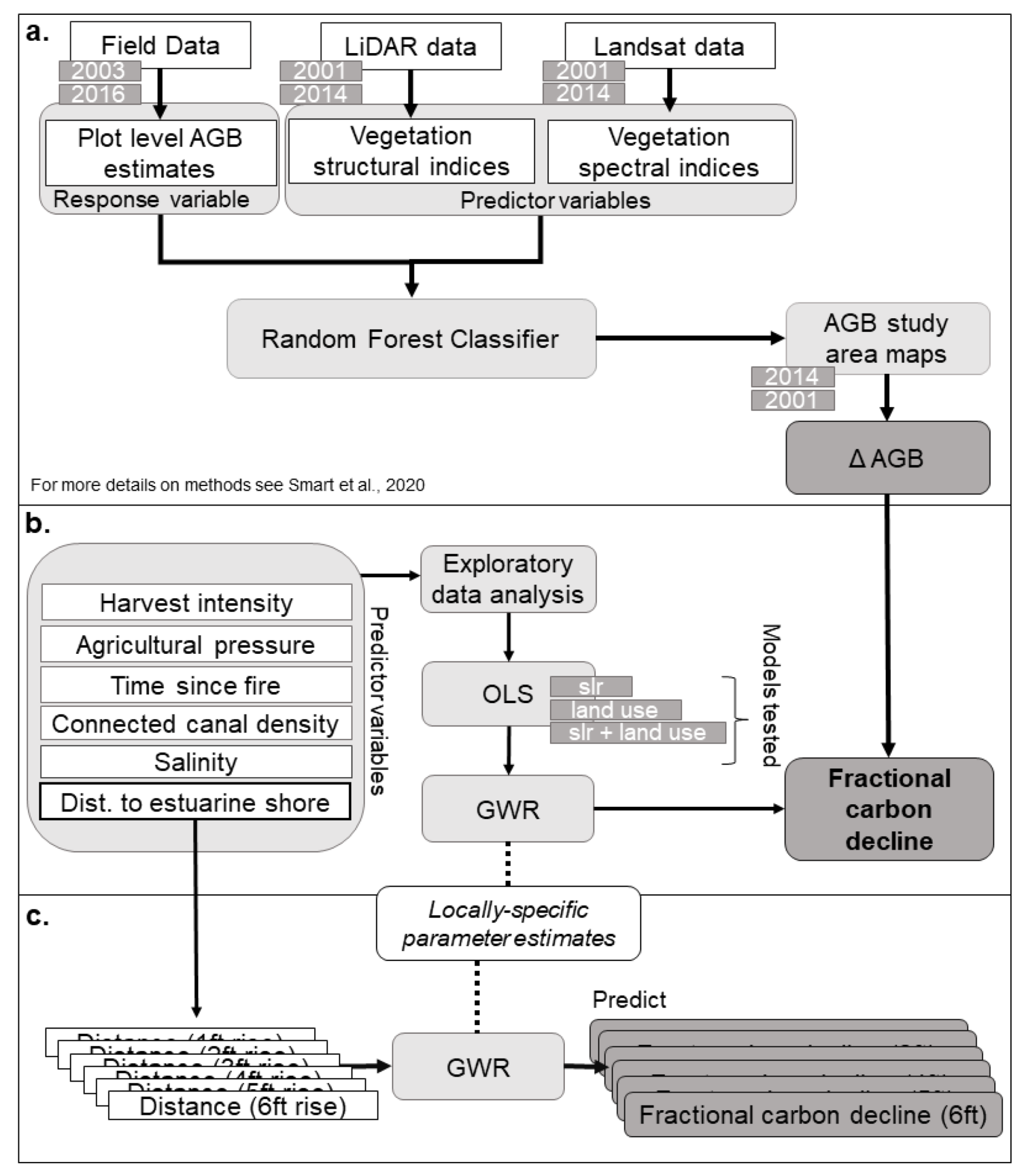
2.2. Mapping Coastal Forest Carbon Declines

We mapped aboveground biomass change between 2001 and 2014 using a combination of field measurements, repeat light detection and ranging (LiDAR) surveys (see Table S1 for specifications) [54,55], and Landsat imagery (see Table S2 for specifications) [49,56]. We quantified vegetation structure and composition with metrics derived from LiDAR and Landsat data for 2001 and 2014 (see Tables S3 and S4 for complete lists of satellite-derived and LiDAR-derived variables). To relate the remote sensing metrics to aboveground biomass, we inventoried the size and density of woody vegetation in 98 plots of 12 m radius [57] across a vegetation gradient from forest to marsh [49]. We calculated total (e.g., woody and herbaceous species) aboveground biomass in megagrams per hectare (Mg ha−1), from these field measurements using established allometric equations [58,59,60] relating diameter at breast height (dbh) or percent cover to total aboveground biomass. We applied the random forest machine learning algorithm (RF; [61]) to quantify relationships between aboveground biomass field measurements and remotely sensed metrics and predict aboveground biomass across the entire study area for 2001 and 2014. RF is an ensemble learning method for classification and regression that functions by constructing many decision trees for model training and then generating mean predictions or the mode of classes across the individual trees. The algorithm corrects for decision trees’ tendency to overfit their training datasets through the bootstrap approach [61]. Using 1000 permutations of the final fitted RF model, we tested model significance, performed validation withholding 30% of the training data, and generated metrics of predictor variable importance. We used the model improvement ratio (MIR) function to select the best predictor variables among the suite of candidate variables, following the methods found in [42]. We then quantified aboveground biomass change by comparing the output maps of aboveground biomass for 2001 and 2014 (Figure 2a and Figure 3a). The RF models performed well (2014 biomass: R2adj. = 0.78, RMSE = 15.0 Mg ha−1, % RMSE = 9.5; 2001 biomass: R2adj. = 0.75, RMSE = 18.3 Mg ha−1, % RMSE = 12.6) [49] (Figure S1). Metrics that contributed most to overall predictive power included mean and median vegetation height, highlighting the importance of vegetation structure for estimating aboveground biomass (Figure S2). We converted aboveground biomass change to carbon loads assuming a carbon concentration of 0.5 [62]. We developed a binary 30-m resolution map of carbon declines, where a value of 1.0 represented any cell with a decrease in carbon over the 13-year period, and a value of 0.0 was assigned to any cell with either no change or an increase in carbon storage. We excluded from the binary map non-vegetated cells and cells classified as developed or agriculture in 2001 or 2014.
Using variogram analysis, we identified 450 m as an appropriate level of aggregation for the response variable (Figure S3). We overlaid the binary carbon decline maps with a 450 × 450-m regular grid and calculated the fraction of the percentage of vegetated area within each modeling unit experiencing carbon declines (Figure 3b).

2.3. Selecting and Mapping Driver Variables

We developed a suite of variables that we expected to be drivers of carbon declines and classified them into different representative classes—land use, natural disturbance, and sea level rise drivers (for complete list, see Table 1).

2.3.1. Land Use Drivers

Land use activities and modifications, such as farming, forestry, and even land abandonment, influence carbon storage and flux on the landscape. Agricultural and forestry pressures (as quantified by agricultural pressure and harvest intensity described below) can alter soil properties, increase nutrient runoff, and change vegetation composition, all of which influence carbon pools both in the areas actively managed and on spatially adjacent or nearby lands [4,9]. Land abandonment (e.g., fallow lands) can also change carbon pools by allowing for natural regeneration, providing buffers from storms for nearby lands, and increasing productivity on site or nearby [51]. Because of their potential to influence carbon fluxes, we included several land use-related variables, derived from spatial datasets, as described in more detail below.
Agricultural and Fallow Pressure.
To account for pressures from agriculture or land abandonment that might influence carbon, we extracted all agricultural lands from the 30-m resolution 2001 National Land Cover Dataset [64] raster and applied a gravity modeling technique, computing for each cell the number of neighboring agricultural cells within a search distance, weighted by a distance decay function [65,66]. This variable accounts for the effect of agricultural lands on nearby forest carbon changes, with more proximate agricultural lands having a stronger influence, as controlled by a coefficient for the distance decay function. For land abandonment, we applied the same methods, extracting instead the fallow land use class from the USDA National Agricultural Statistics Service’s Cropscape dataset [67].
Harvest Intensity.
To identify possible forestry-related land use modifications, we developed a ‘harvest intensity’ metric to quantify changes related to industrial timber harvesting and clearing. We selected the pre-processed annual average Landsat-based Enhanced Vegetation Index (EVI) for every year between 2001 and 2014 from Google Earth Engine [68]. We calculated year-to-year EVI differences and applied a threshold to the average change values to differentiate acute or harvest events from normal variability in EVI based on approximately one standard deviation from the average change values across all year-to-year differences (+/−0.12). We created the ‘harvest intensity index’ by summing all binary rasters created after threshold application; each value in the raster represented the number of times that a cell experienced an acute event during the study period. We removed acute events due to wildfires from the harvest intensity metric because wildfires were accounted for in a separate predictor variable.

2.3.2. Sea Level Rise Drivers

Sea level rise and associated climatic factors can drive changes in carbon storage and flux through a variety of mechanisms [13,14]. To capture general trends or changes in climate, we included climatic variables such as mean precipitation and temperature deviations over the last decade. As climate changes, extreme weather events, such as flooding and hurricanes, are expected to become more frequent and severe [7,25]. Though acute, these events can have lasting impacts on coastal carbon storage—both aboveground and in soils—by altering vegetation and soil composition. These impacts can be compounded by accelerating rates of sea level rise [19,20,29]. To address the potential for these factors to influence carbon flux, we included drivers related to where hurricane storm surges occur (e.g., slow and fast storm surge variables), where water flows and accumulates on the landscape (e.g., elevation, flow direction and accumulation), and proximity to bodies of water (e.g., distance to estuarine shoreline).
Saltwater intrusion, resulting from a combination of both acute events and gradual sea level rise, facilitates changes in vegetation composition and subsequent carbon storage. Long term saltwater exposure in freshwater-dependent forests leads to osmotic stress and eventual mortality [14,20,21]. More salt-tolerant herbaceous species will replace tree species, changing carbon storage capacity, particularly aboveground. Hurricanes and even droughts (by shifting the freshwater–saltwater interface landward) can bring saltwater inland into areas not adapted to saltwater exposure [10,12]. Drainage networks, comprised of canals and ditches, though built to keep water off coastal lands, can serve as conduits during storms, to move water inland [51]. Because salt influences aboveground and soil carbon storage, we included spatial data representing the likelihood of salt impacts by accounting for potential pathways (e.g., the density of canals connected to the estuarine shoreline) and overall salinity values in the adjacent estuary (interpolated from water quality monitoring stations across the landscape). Other factors such as elevation, hurricane storm surge extents, and distance to the estuarine shoreline also indirectly influence where saltwater exposure occurs on the landscape.
Connected Canal Density.
We incorporated hydrological connectivity between coastal forests and the adjacent estuary by extracting artificial drainage features from the US Geological Survey’s National Hydrography Dataset [69]. We removed any isolated canals not connected by other canals or natural water features to the estuarine shoreline. We then calculated the density of linear canal features surrounding each 30-m raster cell using multiple search radii values, ultimately selecting a 1000-m search radius for the final predictor variable.
Salinity.
We used the US Environmental Protection Agency’s STOrage and RETrieval (STORET) database to extract average salinity values (in parts per thousand; ppt) for 3500+ observations from 40 water quality monitoring sites in the Albemarle and Pamlico Sounds between 2001 and 2014 [70]. To interpolate a surface from these point data, we performed an inverse distance weighting interpolation at 30 m resolution [71].

2.3.3. Natural Disturbance Drivers

Frequent, low intensity fires have historically maintained these landscapes [72]. However, catastrophic fires can alter carbon pools by burning the rich organic soils in addition to the vegetation. Though regeneration occurs naturally and rapidly post-fire, interactions between fire, extreme weather events, and climate change can alter carbon storage and flux in unanticipated ways. We included a variable that measures the length of time since a wildfire for the study period to capture these changes in carbon storage and flux.
Time Since Fire.
We used the spatially explicit fire perimeters developed by the Monitoring Trends in Burn Severity Program (MTBS; [73]) and extracted the year of fire attribute to assign the number of years since fire for every fire polygon across the study area.

2.4. Statistical Modeling Approach

We mapped all predictor variables at a 30-m spatial resolution and then aggregated cell values to the spatial modeling unit (450 × 450-m grid cells) via majority (for nominal data) or mean (for continuous data) aggregation methods and derived values for each grid cell. Prior to model fitting, we evaluated predictor variables for multicollinearity and selected a set of uncorrelated (r < 0.5) variables from our initial list (Figure S4). We scaled all variables to values between 0.0 and 1.0 using a minimum–maximum normalization, which retained the original distribution spread but allowed us to evaluate relative contributions of different drivers.
We modeled the relationships between fractional carbon declines and predictor variables using ordinary least squares regression (OLS), a conventional global regression technique, and geographically weighted regression (GWR), a local regression method (Figure 2b). GWR detects heterogeneity in data relationships across geographic space via the fitting of individual localized ordinary least squares regressions [74]. This allows for local variations in rates of change. Coefficients in the model are not global estimates but are specific to a particular location and based on observations taken at sample points near that location [51,75]. The regression equation is then:
y i = α i 0 + k = 1 ,   m α i k x i k + ε i
where y i   is the ith observation of the dependent variable, x i k is the ith observation of the kth independent variable, ε i is the error term, and α i k   is the value of the kth parameter at location 1. Estimates of are then based on observations taken at sample points close to i. A weighting function is then employed so that for each point i there is a bump of influence around i in such a way that those observations near i have more influence in the estimation of parameters than those farther away. In ordinary least squares, the sum of the squared differences of predicted and observed y i   is minimized in the coefficient estimates. In weighted least squares, a weighting factor is applied to each squared difference before minimizing so that the inaccuracy of some predictions carries more of a penalty than others. In weighted regression models the values of the weighting factor are constant so that only one calibration is carried out. In geographically weighted regression, the weighting factor varies with location i so that a different calibration exists for every point in the study area. The geographical weighting is implemented through a spatial kernel function. Common choices for weighting function include Gaussian, bisquare, or tricubic [52]. In addition to the weighting function, a bandwidth is needed that determines the rate of distance decay for each of the data weightings. A large bandwidth smooths parameter estimates, approaching the estimates provided by the global regression, and a small bandwidth tends to sharpen them. The bandwidth can be user-defined or determined using cross-validation (CV) or Akaike’s information criterion (AIC) and can be either a fixed distance or a set number of nearest neighbors (adaptive bandwidth). To minimize potential edge effects, we used an adaptive Gaussian kernel function with an optimal bandwidth selected based on a least squares CV that minimized the squared error. All statistical analyses were carried out using R statistical software and the GWR analyses were performed using the ‘spgwr’ package for R [76,77].
We examined the variance explained by the global and local regression models, Moran’s I tests of model residuals, and the statistical significance and relative importance of predictor variables. We also quantified spatial dependencies and nonstationarity in the relationships between the response and predictor variables by mapping residuals and testing the interquartile ranges of the local coefficient estimates provided by GWR. Additionally, we used the studentized Breusch–Pagan test for heteroscedasticity to identify non-constant variance in the errors. We derived a pseudo-significance test for predictor variables by calculating t-values for each local regression and mapping t-values spatially to identify locations that are statistically significant at alpha = 0.05 [51].

2.5. Predicting Future Coastal Forest Carbon Declines from Sea Level Rise

We used spatial models of future sea level rise inundation from the National Oceanic and Atmospheric Administration (NOAA) to forecast future forest carbon decline [78]. The data depict the potential inundation of coastal areas resulting from a projected 0.3 to 1.8 m sea level rise above current mean higher high water (MHHW) conditions. The values represent the projections for the intermediate to high global mean sea level (GMSL) scenario, which predicts sea levels under Representative Concentration Pathway (RCP) 8.5 from the Intergovernmental Panel on Climate Change (IPCC). This is considered the high-emissions scenario and is referred to as the business-as-usual scenario, which suggests that it is a likely outcome if society does not make concerted efforts to cut greenhouse gas emissions. The model is a function of static elevation and hydrologic connectivity but does not account for other factors such as vertical accretion or subsidence rates, nor does it account for storm surge potential. We calculated total coastal forest carbon loss, measured in teragrams of carbon (TgC), through 2100 by combining our 2014 aboveground carbon maps and the GMSL inundation models. To predict future coastal forest declines in areas not inundated, we updated the distance to the estuarine shoreline predictor variable used in our GWR model using the new estuarine shoreline extent under inundation levels between 0.3 and 1.8 m. Holding all other predictor variables constant, we re-ran the GWR model and examined the resulting predicted fractional carbon declines on the remaining study area (Figure 2c).

3. Results

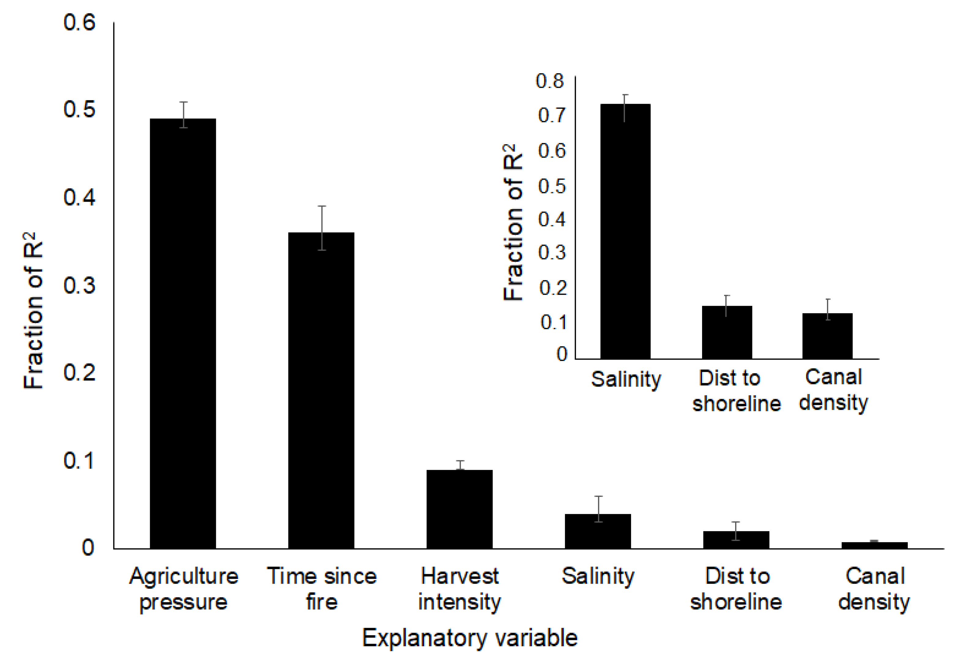
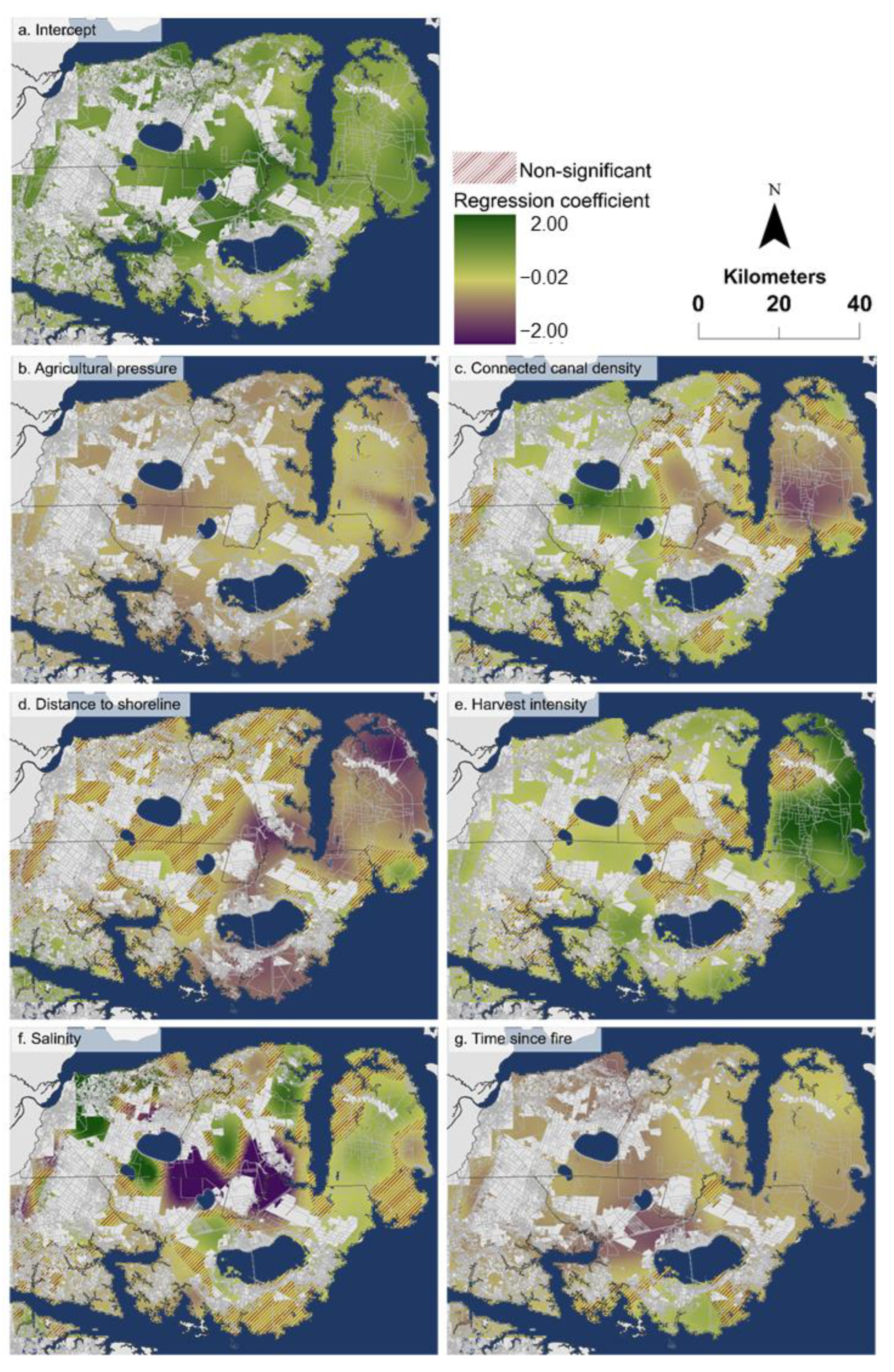
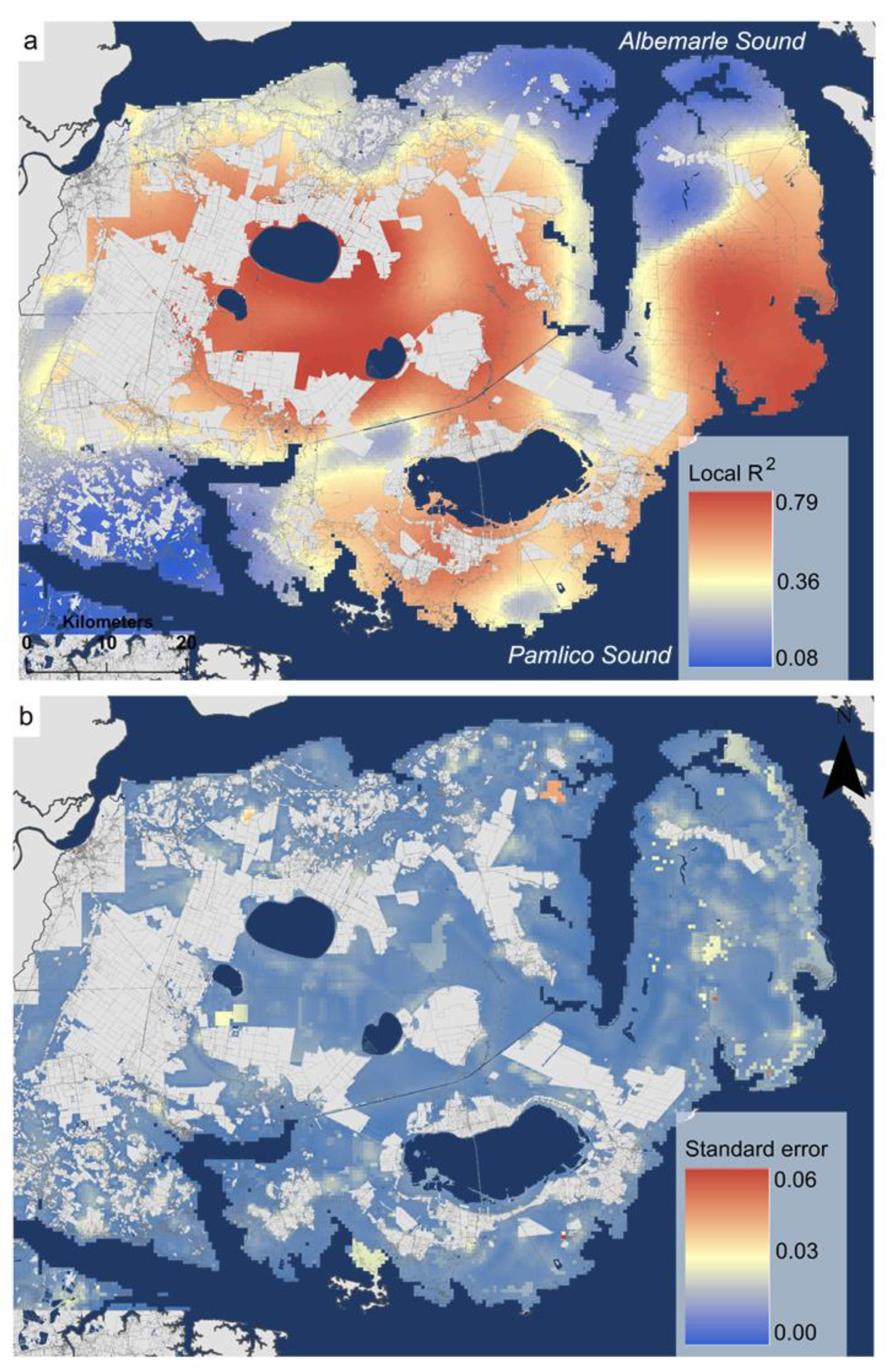
3.1. Statistical Modeling of Coastal Forest Declines

The global regression model explained 39% of the variation in fractional aboveground carbon declines. Statistically significant predictor variables included in the final model were agricultural pressure, connected canal density, time since fire, harvest intensity, distance to shoreline, and salinity (p < 0.05). We found negative relationships between fractional aboveground carbon declines and agricultural pressure, time since fire, and distance to estuarine shoreline. We found positive relationships between fractional aboveground carbon declines and canal density, harvest intensity, and salinity (Table 2).
Land use and disturbance metrics were the most important predictors of variation in fractional carbon decline within the global model, with agricultural pressure explaining the most variation, followed by the time-since-fire variable (Figure 4). Moran’s I tests indicated autocorrelation in the response variable, even at the aggregated 450-m resolution (Moran’s I = 0.75, z-score = 167.77, p-value < 0.0001). The relationship between the predictor variables and the response variable exhibited nonstationarity (Breusch–Pagan statistic = 4092.4, p-value < 0001).
Predictive performance improved with the local regression model, with a lower AIC and higher quasi-global R2. The GWR model explained 52% of the variance, and quasi-global R2 values ranged from 0.08 to 0.79, with more than 50% of the landscape having a local R2 value greater than the global R2 of 0.39 (Figure 5a). Standard errors ranged from a low of 0.006 to a high of 0.06 (Figure 5b). Coefficients for all predictor variables exhibited patterns of spatial non-stationarity according to tests for spatial dependencies (Figure 6).
We found a statistically significant negative relationship between fractional carbon decline and agricultural pressure, canal density, and distance to the estuarine shoreline in the GWR. The range of local coefficient values and statistical significance varied across space, indicating spatial dependencies in the data. On average, we found statistically significant positive relationships between fractional carbon declines and harvest intensity, time since fire, and salinity with spatial heterogeneity in local regression coefficients and statistical significance.
For 52% of the study area, land use and disturbance drivers had the strongest regression coefficients (13% of the total landscape for agricultural pressure, 13% for harvest intensity, and 26% for time since fire), and for 48% of the study area the sea level rise variables had the largest regression coefficients (2% of the total landscape for canal density, 20% for distance to estuarine shoreline, and 27% for salinity). In the southeast portion of the study area, the sea level rise drivers best explained variation in carbon declines (e.g., Figure 6c,d). In the northeast portion of the study area, both land use/disturbance drivers and sea level rise drivers contribute to declines (Figure 6). To the interior, relationships were mixed, with land use drivers most important in areas dominated by agricultural and forestry operations and sea level rise drivers generally most important in interior areas connected to the estuary via canals (e.g., Figure 6b–f).

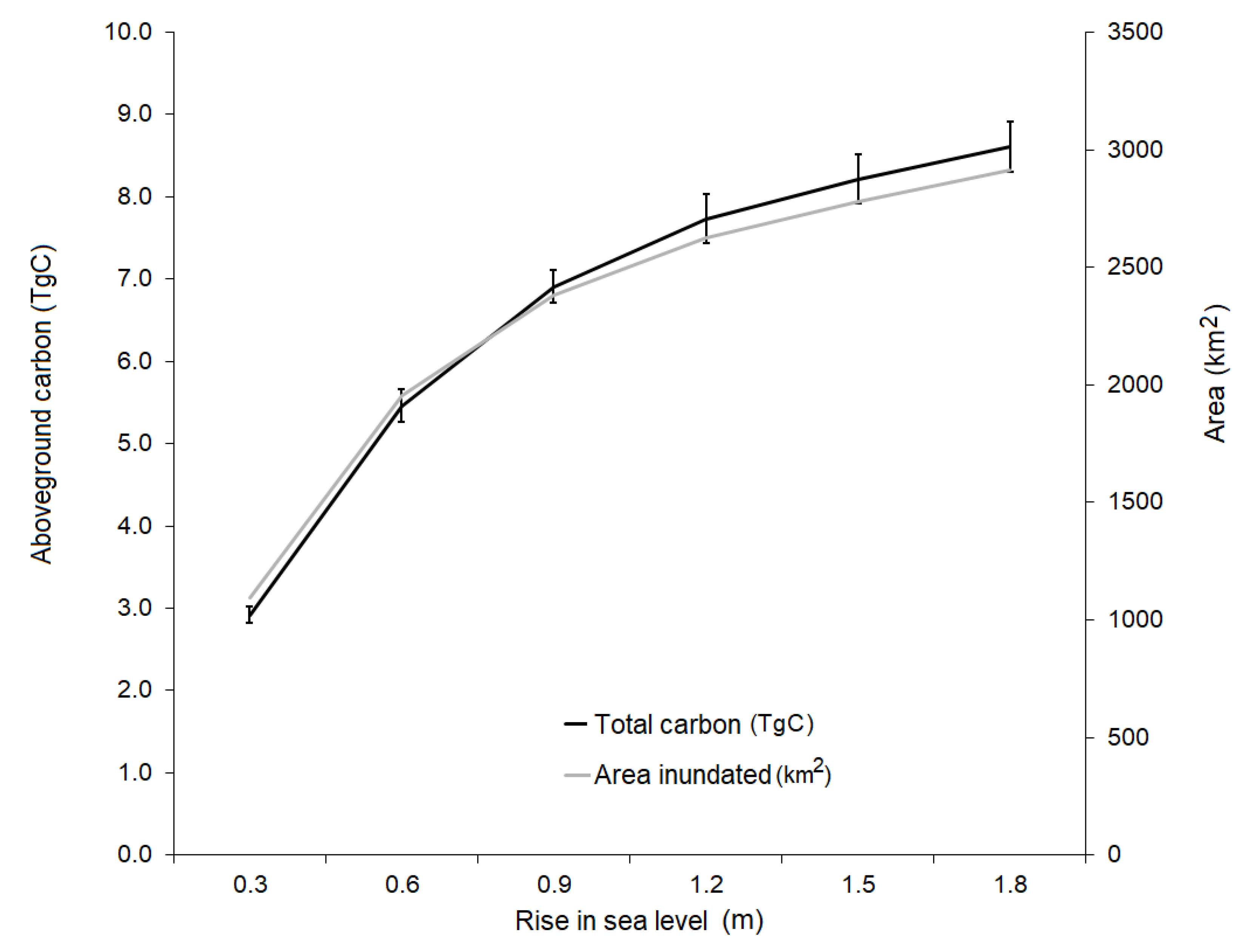
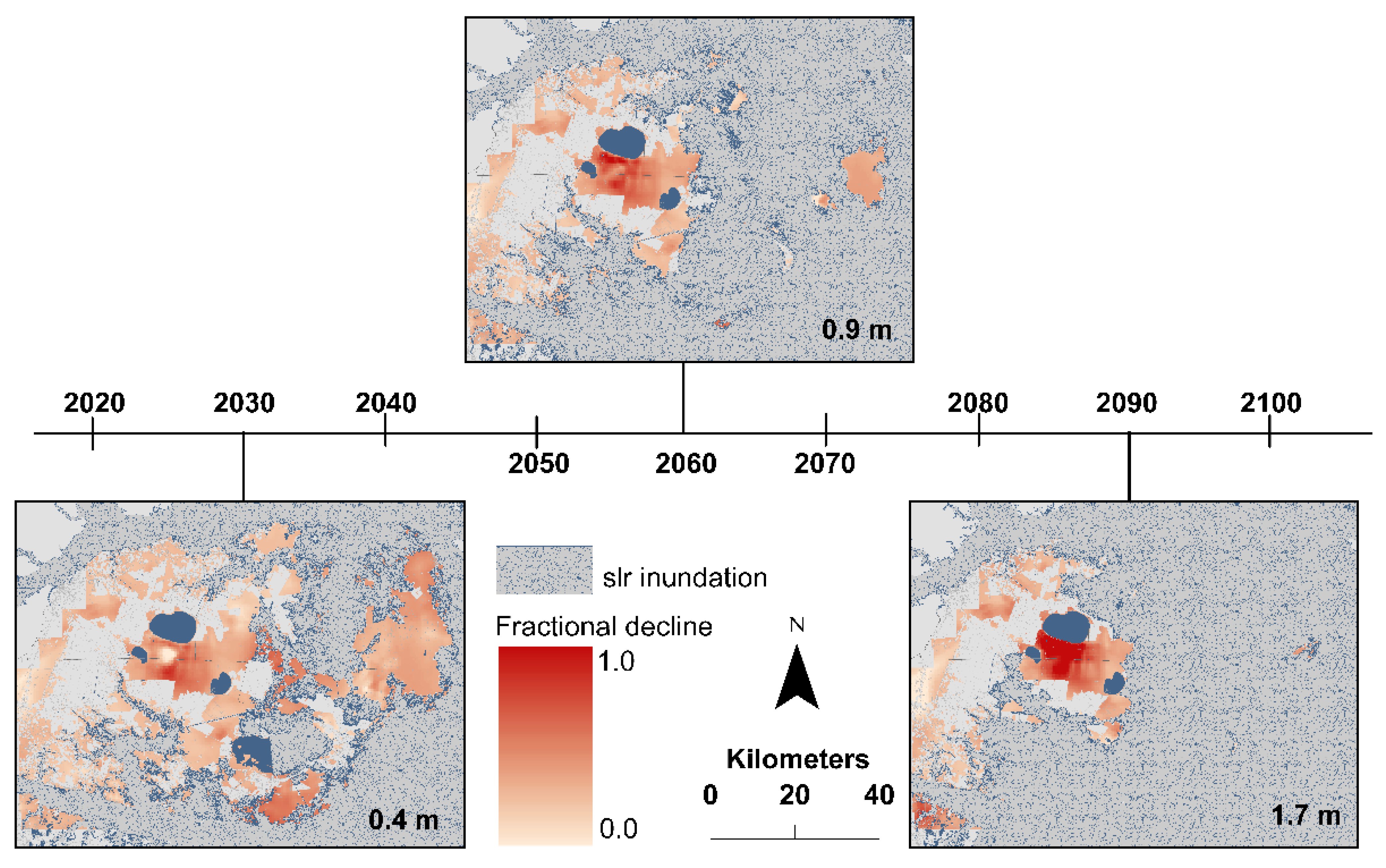
3.2. Future Coastal Forest Declines

We estimated a minimum inundation extent of 1094 km2 for a 0.3 m rise in sea level and a maximum extent of 2914 km2 for a 1.8 m rise in sea level (Figure 7). Associated losses in total aboveground carbon ranged from 2.9 ± 0.1 TgC (0.3 m rise) to 8.6 ± 0.3 TgC (1.8 m rise). On the remaining landscape, we calculated potential declines increasing from 29% to 32% between a 0.3 and 1.8 m rise in sea level. The greatest changes in carbon declines are visible in each scenario adjacent to the shoreline and surrounding the lakes in the study area’s interior (Figure 8).

4. Discussion

Sea level rise, land use activities, and disturbances act synergistically in low-lying coastal forests to alter their structure and function, affecting the ecosystem services they provide. A regional scale understanding of where and how these forests have changed and where to expect future change is critical for prioritizing funding for management and establishing resilient coastal communities. Spatial heterogeneity in the drivers of coastal forest degradation, however, make quantification at regional scales difficult. To address this challenge, we examined the drivers of coastal forest degradation using a local regression approach that accounts for these spatial processes. Using geographically weighted regression (GWR), we examined the relationship between coastal forest fractional carbon declines and land use, disturbance, and sea level rise drivers. We found the patterns of influence to be spatially heterogeneous, providing local insights at regional scales, highlighting the benefit of using a local regression approach to inform management and resource allocation activities more effectively [50,80].
In a low-lying coastal region highly exposed to impacts from sea level rise, we observed that land use and disturbance metrics were the strongest drivers of fractional carbon declines. Agricultural pressure, harvest intensity, and time since fire explained most of the variation in the global model. Interestingly we found a negative relationship between agricultural pressure and fractional carbon declines. Because agricultural lands are generally located at higher elevations in the interior of the study area, the adjacent coastal forests are likely less susceptible to the effects of saltwater intrusion and sea level rise than lower elevation coastal forests near the shore. Alternatively, water control structures, tide gates, and other measures intended to protect the productivity of large-scale agricultural operations may also benefit the coastal forests in these higher elevation areas. In addition to agriculture, approximately 13% of the study area’s inland coastal forests are managed as loblolly pine (Pinus taeda) plantations for timber harvest revenues, which removes a significant amount of aboveground carbon [81]. Though stand-replacing disturbances (e.g., harvests) lead to a net forest C loss, replanting as part of the rotational cycle will eventually replace the lost carbon. However, if trees do not reach maturity and peak primary productivity before subsequent harvests [4,9], increased harvest intensity could result in net carbon losses as was demonstrated in the positive relationship between harvest intensity and aboveground carbon declines in our results.
Natural disturbance events play an important role in coastal forest carbon dynamics. Both the local and global regression models indicated that the time-since-fire metric contributed significantly to the explanatory power of the model, explaining 36% of the model variation. The more recent the fire event, the higher the fractional carbon declines. Despite a low prevalence of prescribed fire and wildfire in our study area compared to historical estimates, fire remains one of the most important drivers of carbon dynamics on the APP [80]. During the study period, several catastrophic wildfires occurred on the Albemarle-Pamlico Peninsula. Though severe wildfires result in aboveground carbon declines, many of the region’s tree species are adapted to fire and regenerate rapidly after fire disturbances [72]. However, if saltwater exposure occurs post-fire, regeneration may be limited by salinity intolerance of the saplings. Accordingly, fire disturbances and saltwater exposure can act synergistically to accelerate forest retreat and facilitate marsh migration of salt-tolerant herbaceous species into the area [19,20].
Although our global regression model indicated sea level rise metrics contributed minimally to the overall explanatory power of the model (explaining only 6.8% of model variation), our local regression model identified places on the landscape where these metrics played a strong and significant role in fractional carbon declines. Distance to the estuarine shoreline, salinity, and connected canal density were important predictors of fractional carbon declines in the northeast and eastern portions of our study area. That there are high levels of spatial heterogeneity in these relationships reinforces the need to consider local spatial regression approaches in dynamic coastal systems. Sea level rise factors are a critical and significant driver of fractional carbon declines, but only near the shoreline and in areas predicted to have high salinities. Unlike the global regression model, our local spatial regression approach can be used to identify the extent and strength of influence for each of these sea level rise drivers in a spatially explicit way. Because the changes associated with saltwater intrusion and sea level rise are likely to be permanent, our approach can be used to identify areas unlikely to recover or return to coastal forest, particularly as sea level rise accelerates. This information can then be used to make more informed decisions about policy, mitigation, and the prioritization of limited resources.
Our results indicate that by 2090, the study area could lose approximately 8.6 TgC of aboveground carbon because of inundation from sea level rise, with the remaining landscape experiencing, on average, 32% fractional declines in carbon. These estimates, however, do not account for future vegetation growth or succession, nor do they consider a potential shift in carbon storage, from aboveground to belowground [2]. This highlights the need to consider impacts on other carbon pools in coastal forests (e.g., soils) and landscape context because shifts in carbon storage in one location alter the amount of carbon stored in another location. Considering these aspects and incorporating potential non-linear relationships, feedbacks, and interactions between natural and anthropogenic drivers via mechanistic or process-based models would provide additional support for targeted adaptation and management activities.
Our study underscores the importance of human interventions in determining future coastal forest resilience. The spatial variation in driving forces of coastal forest degradation has significant implications for prioritizing management activities. Our results indicate that along the shoreline and in the eastern portion of the study area the best management decision might be to facilitate marsh migration, whereas inland there may be more opportunities to work with landowners in conserving or restoring coastal forests. Management of drainage networks, originally built to drain wetlands and lower water tables for agricultural and forestry operations, is another important consideration [81,82]. In the near term these features help mitigate flooding; however, our results from lower elevation coastal forests adjacent to the estuaries suggest that without effective canal and ditch management, these networks act as conduits for saltwater intrusion from extreme weather events and gradual sea level rise [81]. In addition to water management, proactive coastal forest management activities such as lengthened harvest cycles, restricted harvests, and selective harvesting have the potential to enhance the carbon storage and coastal resilience [9]. Selective harvesting and tree species diversification on plantations will also play an important role as sea levels rise and saltwater intrusion increasingly affects forestry operations. Timber harvest revenues can be sustained by harvesting the most at-risk timber (e.g., timber most affected by inundation and saltwater exposure). The common practice of planting a single timber species on plantations increases the likelihood of widespread mortality during extreme storm and flooding events, particularly if that single species is salt-intolerant. Planting a more diverse set of species with a range of salinity tolerances will decrease the severity of impact from extreme storm events and produce added co-benefits associated with increased diversity [83].

5. Conclusions

Our analysis illustrates several key points. First, in a low-lying coastal region highly exposed to impacts from sea level rise, we observed that land use (explaining more than 50% of model variation) and disturbance metrics (explaining 36% of model variation) were the strongest drivers of fractional carbon declines. Second, although our global regression model indicated sea level rise metrics contributed minimally to the overall explanatory power of the model (explaining only 6.8% of model variation), our local regression model identified places on the landscape where these metrics played a strong and significant role in fractional carbon declines. Finally, our results indicate that by 2090, the study area could lose approximately 8.6 TgC of aboveground carbon because of inundation from sea level rise, with the remaining landscape experiencing, on average, 32% fractional declines in carbon. By measuring coastal forest degradation via aboveground carbon storage, we provide an important link to ecosystem services. Because communities may have diverse values for coastal forests, understanding when, where, and how ecosystem services in coastal forests are changing helps managers prioritize resources for management, adaptation, and restoration of coastal ecosystems [84]. Management decisions must consider these trade-offs among ecosystem services as well as current and future susceptibility to land use modifications and sea level rise.
Our approach quantified drivers of coastal forest decline in a spatially explicit way, highlighting the ways that human land use activities, climate, and natural disturbances can act synergistically to alter coastal forest structure and function. By mapping the spatially varying relationships between drivers and carbon declines, we identified geographic locations best suited for targeted management activities. However, to fully understand how these management activities will be implemented, and through what mechanisms, we need a greater understanding of landowner preferences, their evaluation of trade-offs among ecosystem services, their behaviors, and risk perceptions. These are requisite for reducing the uncertainty in coastal forest persistence as sea levels rise.

Supplementary Materials

The following are available online at https://www.mdpi.com/article/10.3390/land10070752/s1, Figure S1: Observed vs. predicted biomass, Figure S2: Predictor variable permutation importance in RF classification, Figure S3: Variogram, Figure S4: Correlation matrix, Table S1: LiDAR flight specifications, Table S2: Landsat imagery specifications, Table S3: Random Forest classification predictor variables; Table S4: Random Forest classification LiDAR predictor variables.

Author Contributions

Conceptualization, L.S.S. and J.W.S.; methodology, L.S.S., J.W.S., K.K.S., P.J.T.; formal analysis, L.S.S.; resources, J.W.S., J.V.; data curation, P.J.T., L.S.S.; writing—original draft preparation, L.S.S.; writing—review and editing, J.W.S., J.V., P.J.T., K.K.S.; funding acquisition, J.W.S. All authors have read and agreed to the published version of the manuscript.

Funding

This research was funded by a joint fellowship through NOAA’s North Carolina Sea Grant Program and NASA’s North Carolina Space Grant Program (NOAA award # NA14OAR4170073, NASA award #NNX15AH81H). Funding from a College of Natural Resources Innovation Grant at NC State University was also used to support this research.

Institutional Review Board Statement

Not applicated.

Informed Consent Statement

Not applicated.

Data Availability Statement

Data generated from this study are available upon request.

Acknowledgments

We are grateful to Joshua Randall from the Center for Geospatial Analytics for edits and comments that greatly improved the quality of this manuscript. We thank Georgina Sanchez of NC State University who provided technical insights during the spatial regression modeling efforts. Additionally, Douglas Newcomb of the US Fish and Wildlife Service provided valuable comments on methods and analyses.

Conflicts of Interest

The authors declare no conflict of interest.

References

  1. Costanza, R.; de Groot, R.; Sutton, P.; Van der Ploeg, S.; Anderson, S.J.; Kubiszewski, I.; Farber, S.; Turner, R.K. Changes in the global value of ecosystem services. Glob. Environ. Chang. 2014, 26, 152–158. [Google Scholar] [CrossRef]
  2. Krauss, K.W.; Noe, G.B.; Duberstein, J.A.; Conner, W.H.; Stagg, C.L.; Cormier, N.; Jones, M.C.; Bernhardt, C.E.; Graeme Lockaby, B.; From, A.S.; et al. The role of the upper tidal estuary in wetland blue carbon storage and flux. Glob. Biogeochem. Cycles 2018, 32, 817–839. [Google Scholar] [CrossRef]
  3. Barbier, E.B.; Hacker, S.D.; Kennedy, C.; Koch, E.W.; Stier, A.C.; Silliman, B.R. The value of estuarine and coastal ecosystem services. Ecol. Monogr. 2011, 81, 169–193. [Google Scholar] [CrossRef]
  4. Aguilos, M.; Mitra, B.; Noormets, A.; Minick, K.; Prajapati, P.; Gavazzi, M.; Sun, G.; McNulty, S.; Li, X.; Domec, J.C.; et al. Long-term carbon flux and balance in managed and natural coastal forested wetlands of the Southeastern USA. Agric. Forest Meteorol. 2020, 288, 108022. [Google Scholar] [CrossRef]
  5. Arkema, K.K.; Verutes, G.M.; Wood, S.A.; Clarke-Samuels, C.; Rosado, S.; Canto, M.; Rosenthal, A.; Ruckelshaus, M.; Guannel, G.; Toft, J.; et al. Embedding ecosystem services in coastal planning leads to better outcomes for people and nature. Proc. Natl. Acad. Sci. USA 2015, 112, 7390–7395. [Google Scholar] [CrossRef] [Green Version]
  6. Enwright, N.M.; Griffith, K.T.; Osland, M.J. Barriers to and opportunities for landward migration of coastal wetlands with sea-level rise. Front. Ecol. Environ. 2016, 14, 307–316. [Google Scholar] [CrossRef]
  7. Kopp, R.E.; Kemp, A.C.; Bittermann, K.; Horton, B.P.; Donnelly, J.P.; Gehrels, W.R.; Hay, C.C.; Mitrovica, J.X.; Morrow, E.D.; Rahmstorf, S. Temperature-driven global sea-level variability in the Common Era. Proc. Natl. Acad. Sci. USA 2016, 113, E1434–E1441. [Google Scholar] [CrossRef] [PubMed] [Green Version]
  8. Jones, M.C.; Bernhardt, C.E.; Krauss, K.W.; Noe, G.B. The impact of late Holocene land use change, climate variability, and sea level rise on carbon storage in tidal freshwater wetlands on the southeastern United States coastal plain. J. Geophys. Res. Biogeosci. 2017, 122, 3126–3141. [Google Scholar] [CrossRef] [Green Version]
  9. Law, B.E.; Hudiburg, T.W.; Berner, L.T.; Kent, J.J.; Buotte, P.C.; Harmon, M.E. Land use strategies to mitigate climate change in carbon dense temperate forests. Proc. Natl. Acad. Sci. USA 2018, 115, 3663–3668. [Google Scholar] [CrossRef] [Green Version]
  10. Ardón, M.; Morse, J.L.; Colman, B.P.; Bernhardt, E.S. Drought-induced saltwater incursion leads to increased wetland nitrogen export. Glob. Chang. Biol. 2013, 19, 2976–2985. [Google Scholar] [CrossRef]
  11. Herbert, E.R.; Boon, P.; Burgin, A.J.; Neubauer, S.C.; Franklin, R.B.; Ardón, M.; Hopfensperger, K.N.; Lamers, L.P.; Gell, P. A global perspective on wetland salinization: Ecological consequences of a growing threat to freshwater wetlands. Ecosphere 2015, 6, 1–43. [Google Scholar] [CrossRef]
  12. Ardón, M.; Helton, A.M.; Bernhardt, E.S. Drought and saltwater incursion synergistically reduce dissolved organic carbon export from coastal freshwater wetlands. Biogeochemistry 2016, 127, 411–426. [Google Scholar] [CrossRef]
  13. Mcleod, E.; Chmura, G.L.; Bouillon, S.; Salm, R.; Björk, M.; Duarte, C.M.; Lovelock, C.E.; Schlesinger, W.H.; Silliman, B.R. A blueprint for blue carbon: Toward an improved understanding of the role of vegetated coastal habitats in sequestering CO2. Front. Ecol. Environ. 2011, 9, 552–560. [Google Scholar] [CrossRef] [Green Version]
  14. Henman, J.; Poulter, B. Inundation of freshwater peatlands by sea level rise: Uncertainty and potential carbon cycle feedbacks. J. Geophys. Res. Biogeosci. 2008, 113. [Google Scholar] [CrossRef]
  15. Chmura, G.L.; Anisfeld, S.C.; Cahoon, D.R.; Lynch, J.C. Global carbon sequestration in tidal, saline wetland soils. Glob. Biogeochem. Cycles 2003, 17. [Google Scholar] [CrossRef]
  16. Donato, D.C.; Kauffman, J.B.; Murdiyarso, D.; Kurnianto, S.; Stidham, M.; Kanninen, M. Mangroves among the most carbon-rich forests in the tropics. Nat. Geosci. 2011, 4, 293. [Google Scholar] [CrossRef]
  17. Loder, A.L.; Finkelstein, S.A. Carbon accumulation in freshwater marsh soils: A synthesis for temperate North America. Wetlands 2020, 40, 1173–1187. [Google Scholar] [CrossRef]
  18. Williams, K.; Ewel, K.C.; Stumpf, R.P.; Putz, F.E.; Workman, T.W. Sea-level rise and coastal forest retreat on the west coast of Florida, USA. Ecology 1999, 80, 2045–2063. [Google Scholar] [CrossRef]
  19. Poulter, B.; Qian, S.S.; Christensen, N.L. Determinants of coastal treeline and the role of abiotic and biotic interactions. Plant Ecol. 2009, 202, 55–66. [Google Scholar] [CrossRef]
  20. Desantis, L.R.; Bhotika, S.; Williams, K.; Putz, F.E. Sea-level rise and drought interactions accelerate forest decline on the Gulf Coast of Florida, USA. Glob. Chang. Biol. 2007, 13, 2349–2360. [Google Scholar] [CrossRef]
  21. Brinson, M.M.; Christian, R.R.; Blum, L.K. Multiple states in the sea-level induced transition from terrestrial forest to estuary. Estuaries 1995, 18, 648–659. [Google Scholar] [CrossRef]
  22. Moorhead, K.K.; Brinson, M.M. Response of wetlands to rising sea level in the lower coastal plain of North Carolina. Ecol. Appl. 1995, 5, 261–271. [Google Scholar] [CrossRef]
  23. Kirwan, M.L.; Gedan, K.B. Sea-level driven land conversion and the formation of ghost forests. Nat. Clim. Chang. 2019, 9, 450–457. [Google Scholar] [CrossRef] [Green Version]
  24. Sallenger, A.H.; Doran, K.S.; Howd, P.A. Hotspot of accelerated sea-level rise on the Atlantic coast of North America. Nat. Clim. Chang. 2012, 2, 884–888. [Google Scholar] [CrossRef]
  25. Sweet, W.V.; Marra, J.J. 2015 State of U.S. Nuisance Tidal Flooding. Supplement to State of the Climate: National Overview for May 2016; National Oceanic and Atmospheric Administration, National Centers for Environmental Information: Asheville, NC, USA, 2016; p. 5. Available online: https://www.ncdc.noaa.gov/monitoring-content/sotc/national/2016/may/sweet-marra-nuisance-flooding-2015.pdf (accessed on 1 December 2018).
  26. Karegar, M.A.; Dixon, T.H.; Engelhart, S.E. Subsidence along the Atlantic Coast of North America: Insights from GPS and late Holocene relative sea level data. Geophys. Res. Lett. 2016, 43, 3126–3133. [Google Scholar] [CrossRef] [Green Version]
  27. Poulter, B.; Halpin, P.N. Raster modelling of coastal flooding from sea-level rise. Int. J. Geogr. Inf. Sci. 2008, 22, 167–182. [Google Scholar] [CrossRef]
  28. Field, C.R.; Dayer, A.A.; Elphick, C.S. Landowner behavior can determine the success of conservation strategies for ecosystem migration under sea-level rise. Proc. Natl. Acad. Sci. USA 2017, 114, 9134–9139. [Google Scholar] [CrossRef] [Green Version]
  29. White, E.; Kaplan, D. Restore or retreat? Saltwater intrusion and water management in coastal wetlands. Ecosyst. Health Sustain. 2017, 3, e01258. [Google Scholar] [CrossRef] [Green Version]
  30. Stagg, C.L.; Baustian, M.M.; Perry, C.L.; Carruthers, T.J.; Hall, C.T. Direct and indirect controls on organic matter decomposition in four coastal wetland communities along a landscape salinity gradient. J. Ecol. 2018, 106, 655–670. [Google Scholar] [CrossRef]
  31. Fatoyinbo, T.; Feliciano, E.A.; Lagomasino, D.; Lee, S.K.; Trettin, C. Estimating mangrove aboveground biomass from airborne LiDAR data: A case study from the Zambezi River delta. Environ. Res. Lett. 2018, 13, 025012. [Google Scholar] [CrossRef] [Green Version]
  32. Klemas, V.V. Remote sensing of landscape-level coastal environmental indicators. Environ. Manag. 2001, 27, 47–57. [Google Scholar] [CrossRef] [PubMed]
  33. DeFries, R.S.; Houghton, R.A.; Hansen, M.C.; Field, C.B.; Skole, D.; Townshend, J. Carbon emissions from tropical deforestation and regrowth based on satellite observations for the 1980s and 1990s. Proc. Natl. Acad. Sci. USA 2002, 99, 14256–14261. [Google Scholar] [CrossRef] [PubMed] [Green Version]
  34. Byrd, K.B.; O’Connell, J.L.; Di Tommaso, S.; Kelly, M. Evaluation of sensor types and environmental controls on mapping biomass of coastal marsh emergent vegetation. Remote Sens. Environ. 2014, 149, 166–180. [Google Scholar] [CrossRef]
  35. Lefsky, M.; Warren, B.; Hardings, D.J.; Parker, G.G.; Ackery, S.A.; Gower, S.T. Lidar remote sensing of above-ground biomass in three biomes. Environ. Res. 2002, 11, 393–399. [Google Scholar] [CrossRef] [Green Version]
  36. Lim, K.; Treitz, P.; Baldwin, K.; Morrison, I.; Green, J. Lidar remote sensing of biophysical properties of tolerant northern hardwood forests. Can. J. Remote Sens. 2003, 29, 658–678. [Google Scholar] [CrossRef]
  37. Anderson, J.; Martin, M.E.; Smith, M.-L.; Dubayah, R.O.; Hofton, M.A.; Hyde, P.; Peterson, B.E.; Blair, J.B.; Knox, R.G. The use of waveform lidar to measure northern temperate mixed conifer and deciduous forest structure in New Hampshire. Remote Sens. Environ. 2006, 105, 248–261. [Google Scholar] [CrossRef]
  38. Fatoyinbo, T.E.; Simard, M. Height and biomass of mangroves in Africa from ICESat/GLAS and SRTM. Int. J. Remote Sens. 2013, 34, 668–681. [Google Scholar] [CrossRef]
  39. Sexton, J.O.; Bax, T.; Siqueira, P.; Swenson, J.J.; Hensley, S. A comparison of lidar, radar, and field measurements of canopy height in pine and hardwood forests of southeastern North America. For. Ecol. Manag. 2009, 257, 1136–1147. [Google Scholar] [CrossRef]
  40. Riegel, J.B.; Bernhardt, E.; Swenson, J. Estimating above-ground Carbon Biomass in a Newly Restored Coastal Plain Wetland Using Remote Sensing. PLoS ONE 2013, 8, e68251. [Google Scholar] [CrossRef]
  41. Kulawardhana, R.W.; Popescu, S.C.; Feagin, R.A. Fusion of lidar and multispectral data to quantify salt marsh carbon stocks. Remote Sens. Environ. 2014, 154, 345–357. [Google Scholar] [CrossRef]
  42. Hudak, A.T.; Strand, E.K.; Vierling, L.A.; Byrne, J.C.; Eitel, J.U.H.; Martinuzzi, S.; Falkowski, M.J. Quantifying aboveground forest carbon pools and fluxes from repeat LiDAR surveys. Remote Sens. Environ. 2012, 123, 25–40. [Google Scholar] [CrossRef] [Green Version]
  43. Økseter, R.; Bollandsås, O.M.; Gobakken, T.; Næsset, E. Modeling and predicting aboveground biomass change in young forest using multi-temporal airborne laser scanner data. Scand. J. For. Res. 2015, 30, 458–469. [Google Scholar] [CrossRef]
  44. Cao, L.; Coops, N.C.; Innes, J.L.; Sheppard, S.R.J.; Fu, L.; Ruan, H.; She, G. Estimation of forest biomass dynamics in subtropical forests using multi-temporal airborne LiDAR data. Remote Sens. Environ. 2016, 178, 158–171. [Google Scholar] [CrossRef]
  45. Hudak, A.T.; Fekety, P.A.; Kane, V.R.; Kennedy, R.E.; Filippelli, S.K.; Falkowski, M.J.; Tinkham, W.T.; Smith, A.M.; Crookston, N.L.; Domke, G.M.; et al. A carbon monitoring system for mapping regional, annual aboveground biomass across the northwestern USA. Environ. Res. Lett. 2020, 15, 095003. [Google Scholar] [CrossRef]
  46. Byrd, K.B.; Windham-Myers, L.; Leeuw, T.; Downing, B.; Morris, J.T.; Ferner, M.C. Forecasting tidal marsh elevation and habitat change through fusion of Earth observations and a process model. Ecosphere 2016, 7, e01582. [Google Scholar] [CrossRef]
  47. Hamilton, S.E.; Friess, D.A. Global carbon stocks and potential emissions due to mangrove deforestation from 2000 to 2012. Nat. Clim. Chang. 2018, 8, 240–244. [Google Scholar] [CrossRef] [Green Version]
  48. Lagomasino, D.; Fatoyinbo, T.; Lee, S.; Feliciano, E.; Trettin, C.; Shapiro, A.; Mangora, M.M. Measuring mangrove carbon loss and gain in deltas. Environ. Res. Lett. 2019, 14, 025002. [Google Scholar] [CrossRef]
  49. Smart, L.S.; Taillie, P.J.; Poulter, B.; Vukomanovic, J.; Singh, K.K.; Swenson, J.J.; Mitasova, H.; Smith, J.W.; Meentemeyer, R.K. Aboveground carbon loss associated with the spread of ghost forests as sea levels rise. Environ. Res. Lett. 2020, 15, 104028. [Google Scholar] [CrossRef]
  50. Foody, G.M. Spatial nonstationarity and scale-dependency in the relationship between species richness and environmental determinants for the sub-Saharan endemic avifauna. Glob. Ecol. Biogeogr. 2004, 13, 315–320. [Google Scholar] [CrossRef]
  51. Fotheringham, S.; Brundson, C.; Charlton, M. Geographically Weighted Regression & Associated Techniques; John Wiley & Sons: West Sussex, UK, 2003. [Google Scholar]
  52. Mason, S.A.; Olander, L.P.; Grala, R.K.; Galik, C.S.; Gordon, J.S. A practice-oriented approach to foster private landowner participation in ecosystem service conservation and restoration at a landscape scale. Ecosyst. Serv. 2020, 46, 101203. [Google Scholar] [CrossRef]
  53. Bhattachan, A.; Jurjonas, M.D.; Moody, A.C.; Morris, P.R.; Sanchez, G.M.; Smart, L.S.; Taillie, P.J.; Emanuel, R.E.; Seekamp, E.L. Sea level rise impacts on rural coastal social-ecological systems and the implications for decision making. Environ. Sci. Policy 2018, 90, 122–134. [Google Scholar] [CrossRef]
  54. National Oceanic and Atmospheric Administration (NOAA). 2001 NCFMP Lidar: Phase. 2012. Available online: https://chs.coast.noaa.gov/htdata/lidar1_z/geoid18/data/1397/ (accessed on 1 December 2016).
  55. National Oceanic and Atmospheric Administration (NOAA). 2014 NCFMP Lidar: Phase. 2014. Available online: https://chs.coast.noaa.gov/htdata/lidar1_z/geoid18/data/4954/ (accessed on 1 December 2016).
  56. US Geographical Survey (USGS). 2018 GloVis Data Warehouse. Available online: http://glovis.usgs.gov (accessed on 15 December 2016).
  57. Taillie, P.J.; Moorman, C.E.; Poulter, B.; Ardón, M.; Emanuel, R.E. Decadal-scale vegetation change driven by salinity at leading edge of rising sea level. Ecosystems 2019, 22, 1918–1930. [Google Scholar] [CrossRef]
  58. Smith, W.B.; Brand, G.J. Allometric biomass equations for 98 species of herbs, shrubs, and small trees. In Research Note NC-299; US Dept. of Agriculture, Forest Service, North Central Forest Experiment Station, 299: St. Paul, MN, USA, 1983. [Google Scholar]
  59. Jenkins, J.C.; Chojnacky, D.C.; Heath, L.S.; Birdsey, R.A. National-scale biomass estimators for United States tree species. For. Sci. 2003, 49, 12–35. [Google Scholar]
  60. Castillo, J.M.; Leira-Doce, P.; Rubio-Casal, A.E.; Figueroa, E. Spatial and temporal variations in aboveground and belowground biomass of Spartina maritima (small cordgrass) in created and natural marshes. Estuar. Coast. Shelf Sci. 2008, 78, 819–826. [Google Scholar] [CrossRef]
  61. Breiman, L. Random Forests. Mach. Learn. 2001, 45, 5–32. [Google Scholar] [CrossRef] [Green Version]
  62. Martin, A.R.; Doraisami, M.; Thomas, S.C. Global patterns in wood carbon concentration across the world’s trees and forests. Nat. Geosci. 2018, 11, 915–920. [Google Scholar] [CrossRef]
  63. National Ocean Service. Tides and Currents: Bench Mark Sheet for 8651370 2017, Duck NC. Available online: https://tidesandcurrents.noaa.gov/benchmarks.html?id=8651370 (accessed on 1 January 2018).
  64. MRLC. Multi-Resolution Land Characteristics Consortium: National Land Cover Database (NLCD) 2001. 2017. Available online: https://www.mrlc.gov/data?f%5B0%5D=category%3Aland%20cover&f%5B1%5D=year%3A2016 (accessed on 1 January 2017).
  65. Meentemeyer, R.K.; Tang, W.; Dorning, M.A.; Vogler, J.B.; Cunniffe, N.J.; Shoemaker, D.A. Futures: Multilevel simulations of emerging urban–rural landscape structure using a stochastic patch-growing algorithm. Ann. Assoc. Am. Geogr. 2013, 103, 785–807. [Google Scholar] [CrossRef] [Green Version]
  66. GRASS Development Team. Geographic Resources Analysis Support System (GRASS) Software, Version 7.2; Open Source Geospatial Foundation: Chicago, IL, USA, 2017; Available online: https://grass.osgeo.org/ (accessed on 1 January 2017).
  67. US Department of Agriculture (USDA). National Agricultural Statistics Service Cropland Data Layer: Published Crop-Specific Data Layer. 2018. Available online: https://nassgeodata.gmu.edu/CropScape/ (accessed on 1 December 2017).
  68. Google Earth Engine. A Planetary-Scale Platform for Earth Science Data & Analysis. 2018. Available online: https://earthengine.google.com/ (accessed on 1 December 2017).
  69. US Geological Survey (USGS). National Hydrography Geodatabase: The National Map Viewer. 2013. Available online: http://nhd.usgs.gov/data.html (accessed on 15 May 2016).
  70. US Environmental Protection Agency (US EPA). 2017 STORage and RETrieval Warehouse/Water Quality Exchange. Available online: www3.epa.gov/storet/bck/dbtop.html (accessed on 1 January 2017).
  71. Emadi, M.; Baghernejad, M. Comparison of spatial interpolation techniques for mapping soil pH and salinity in agricultural coastal areas, northern Iran Arch. Agron. Soil Sci. 2014, 60, 1315–1327. [Google Scholar] [CrossRef]
  72. Frost, C.C. Presettlement fire regimes in southeastern marshes, peatlands, and swamps. In Proceedings of the 19th Tall Timbers Fire Ecology Conference: Fire in Wetlands: A Management Perspective, Tallahassee, FL, USA, 1995; Tall Timbers Research Inc.: Tallahassee, FL, USA, 1995. Available online: http://talltimbers.org/wp-content/uploads/2014/03/Frost1995_op.pdf (accessed on 23 August 2016).
  73. US Forest Service (USFS); US Geological Survey (USGS). Monitoring Trends in Burn Severity (MTBS) Data Access: Fire Level Geospatial Data. 2017. Available online: http://mtbs.gov/direct-download (accessed on 1 May 2017).
  74. Harris, P.; Fotheringham, A.S.; Crespo, R.; Charlton, M. The use of geographically weighted regression for spatial prediction: An evaluation of models using simulated data sets. Math. Geosci. 2010, 42, 657–680. [Google Scholar] [CrossRef]
  75. Brunsdon, C.; Fotheringham, S.; Charlton, M. Geographically weighted regression. J. R. Stat. Soc. Ser. D 1998, 47, 431–443. [Google Scholar] [CrossRef]
  76. R Core Development Team. R: A Language and Environment for Statistical Computing; R Foundation for Statistical Computing: Vienna, Austria, 2018; Available online: https://www.R-project.org/ (accessed on 10 January 2018).
  77. Bivand, R.; Yu, D.; Nakaya, T.; Garcia-Lopez, M.A.; Bivand, M.R. Packag ‘Spgwr’. R Software Package. 2017. Available online: https://cran.r-project.org/web/packages/spgwr/index.html (accessed on 10 January 2018).
  78. NOAA Office for Coastal Management (NOAA OCM). Sea Level Rise Data Download. 2017. Available online: https://coast.noaa.gov/slrdata/ (accessed on 1 December 2017).
  79. Lindeman, R.H.; Merenda, P.F.; Gold, R.Z. Introduction to Bivariate and Multivariate Analysis; Scott, Foresman: Glenview, IL, USA, 1980. [Google Scholar]
  80. Su, S.; Li, D.; Xiao, R.; Zhang, Y. Spatially non-stationary response of ecosystem service value changes to urbanization in Shanghai, China. Ecol. Indic. 2014, 45, 332–339. [Google Scholar] [CrossRef]
  81. Bhattachan, A.; Emanuel, R.E.; Ardon, M.; Bernhardt, E.S.; Anderson, S.M.; Stillwagon, M.G.; Ury, E.A.; Bendor, T.K.; Wright, J.P. Evaluating the effects of land-use change and future climate change on vulnerability of coastal landscapes to saltwater intrusion. Elem. Sci. Anthr. 2018, 6, 62. [Google Scholar] [CrossRef] [Green Version]
  82. Poulter, B.; Goodall, J.L.; Halpin, P.N. Applications of network analysis for adaptive management of artificial drainage systems in landscapes vulnerable to sea level rise. J. Hydrol. 2008, 357, 207–217. [Google Scholar] [CrossRef]
  83. Tully, K.; Gedan, K.; Epanchin-Niell, R.; Strong, A.; Bernhardt, E.S.; BenDor, T.; Mitchell, M.; Kominoski, J.; Jordan, T.E.; Neubauer, S.C.; et al. The invisible flood: The chemistry, ecology, and social implications of coastal saltwater intrusion. BioScience 2019, 69, 368–378. [Google Scholar] [CrossRef]
  84. Rodrigues, J.G.; Conides, A.J.; Rivero Rodriguez, S.; Raicevich, S.; Pita, P.; Kleisner, K.M.; Pita, C.; Lopes, P.F.; Alonso Roldáni, V.; Ramos, S.S.; et al. Marine and coastal cultural ecosystem services: Knowledge gaps and research priorities. One Ecosyst. 2017, 2, e12290. [Google Scholar] [CrossRef]
Figure 1. The Albemarle-Pamlico Peninsula is an approximately 4000 km2 region in Eastern North Carolina, USA. It is bounded by the Albemarle and Pamlico Sounds, which are separated from the Atlantic Ocean by a chain of barrier islands. Almost half (47%) of the peninsula lies below 1 m in elevation exposing agricultural lands, forestry operations, and natural coastal forests to impacts from sea level rise.
Land 10 00752 g001
Figure 2. Schematic describing the three main analyses that include (a) mapping aboveground biomass (AGB) change and calculating fractional carbon decline (Section 2.2; for more details on methods [49]); (b) exploratory data analysis to select uncorrelated predictor variables and modeling fractional carbon decline as a function of sea level rise (slr), land-use, or a combination of drivers using nonspatial (ordinary least squares; OLS) and spatial (geographically weighted regression; GWR) regression models (Section 2.3 and Section 2.4); and (c) using the locally specific parameter estimates established from the GWR model to predict future fractional carbon declines by holding all other variables constant and updating the distance to estuarine shoreline variable (Section 2.5).
Land 10 00752 g002
Figure 3. (a) Aboveground biomass change, measured as Mg ha −1, between 2001 and 2014, for the Albemarle-Pamlico study area in Eastern North Carolina. Areas excluded from the model are in light grey. Water bodies and the Albemarle and Pamlico Sounds are dark blue. (b) Fractional carbon decline, calculated from (a) by converting 30-m grid cells to carbon loads, developing a binary 30-m resolution map by assigning carbon declines values of 1, and aggregating data to 450 × 450-m grid. Fractional carbon decline is the fraction (see inset schematic; purple cells divided by green cells; 0.33) of the percentage of vegetation area (colored cells divided by total number of cells; 0.67) within each 450 × 450-m modeling unit experiencing decline.
Land 10 00752 g003
Figure 4. Relative importance for each predictor variable used in the final model (R2 = 0.39) with 95% bootstrap confidence intervals using the method from [79]. Metrics are normalized to sum to 100%. Inset shows the relative importance of predictor variables for a model that includes only the sea level rise drivers (R2 = 0.05).
Land 10 00752 g004
Figure 5. (a) Quasi-global R2 from geographically weighted regression (GWR) model for the Albemarle-Pamlico study area in Eastern North Carolina, USA. Areas excluded from the model are in light grey. Water bodies and the Albemarle and Pamlico Sounds are dark blue. (b) Quasi-global R2 standard error values from the GWR model.
Land 10 00752 g005
Figure 6. (ag) Coefficients for intercept and predictor variables used in the final geographically weighted regression model for the Albemarle-Pamlico study area in Eastern North Carolina, USA. Areas excluded from the model are in light grey. Water bodies and the Albemarle and Pamlico Sounds are dark blue. Red diagonal lines indicate locations where the predictor variables were not statistically significant in the local regression models according to the pseudo-significance tests.
Land 10 00752 g006
Figure 7. Total area (km2) inundated (grey line; right axis) and total aboveground carbon, measured in teragrams of carbon (TgC), lost (black line; left axis) and associated standard errors from sea level rise inundation. The sea level rise inundation model, from the National Oceanic and Atmospheric Administration, represents inundation under the intermediate–high sea level rise (slr) scenario (ranging from 0.3 to 1.8 m) or Representative Concentration Pathway 8.5.
Land 10 00752 g007
Figure 8. Fractional carbon declines associated with sea level rise inundation using the National Oceanic and Atmospheric Administration’s Sea level rise (slr) inundation models for the intermediate–high sea level rise inundation scenario (values range from 0.3 to 1.8 m). Fractional carbon declines estimated using the geographically weighted regression model with distance to estuarine shoreline predictor variable updated with incremental inundation between 0.3 and 1.8 m.
Land 10 00752 g008
Table 1. Suite of spatially explicit predictor variables explored within the land use, natural disturbance, and sea level rise categories. All variables were developed as 30-m resolution raster datasets and aggregated using a 450 × 450-m grid.
Description Base DataYearData Source
Land Use Drivers
Agricultural pressureGravity model, number of neighboring agriculture cells within a search distance and weighted by distance CDL, Cropscape2001, 2014 NASS
Fallow pressureGravity model, number of neighboring fallow cells within a search distance and weighted by distance CDL, Cropscape2001, 2014 NASS
Harvest intensityThreshold applied to between-year mean NDVI change to create binary outputs of harvest/acute event, summed across yearsNDVI2001–2014Google Earth Engine
Natural Disturbance Drivers
Time since fireUsing fire perimeters and year of fire, assigned number of years since fire across the landscapeVector fileCurrent MTBS
Sea Level Rise Drivers
Connected canal density Line density of only those canals connected to open water in study area, with influence at 1000 m distance NHD Current USGS
Distance to estuarine shoreline Euclidean distance (km) to estuarine shoreline NHD Current USGS
Fast storm surge Fast storm surge categories Vector file Current NC Onemap
Flow accumulationFlow accumulation DEM2014Derived
Flow directionFlow directionDEM2014Derived
Salinity Inverse distance weighting interpolation of average salinity (ppt) from 2001 to 2014 STORET 2001–2014EPA
Mean precipitation deviationYearly (2001–2014) average precipitation difference (mm) from historical norm (1990–2000) 2001–2014Google Earth Engine
MHHW adjusted elevation *Elevation (m) adjusted by current mean higher high water (MHHW) MHHW, DEM2014Derived
Minimum temperature deviationYearly (2001–2014) minimum temperature difference (degrees Celsius) from historical norm (1990–2000) 2001–2014Google Earth Engine
Slow storm surge Slow storm surge categories Vector file Current NC Onemap
Note: Monitoring Trends in Burn Severity Program (MTBS), National Agricultural Statistics Service (NASS), US Environmental Protection Agency (EPA), US Geological Survey (USGS) digital elevation model (DEM), National Hydrography Dataset (NHD), normalized difference vegetation index (NDVI). * Mean higher high water (MHHW) is the average of the higher high water height of each tidal day over the National Tidal Datum Epoch. The station on Duck Pier in North Carolina, USA, was used as our reference and for the current National Tidal Datum Epoch (1983–2001); their MHHW is 1.24 m [63].
Table 2. (a) Coefficient and standard errors for predictor variables used in the global ordinary least squares (OLS) regression model. (b) Coefficient mean (and range) and standard error mean (and range) for the local geographically weighted regression (GWR) model. + denotes nonstationarity in the relationship between predictor variable and response in the GWR model as calculated by the Breusch–Pagan statistic.
(a) OLS(b) GWR
CoefficientStandard ErrorCoefficient Mean
(Range)
Standard Error Mean
(Range)
Intercept ***+0.8910.0090.825
(0.120, 1.765)
0.054
(0.026, 0.273)
Agricultural pressure ***+−0.4310.006−0.387
(−1.140, −0.075)
0.029
(0.015, 0.232)
Connected canal density ***+0.0840.0130.168
(−1.308, 1.629)
0.075
(0.026, 0.198)
Time since fire ***+−0.4710.007−0.398
(−1.250, 0.507)
0.048
(0.014, 0.311)
Harvest intensity ***+0.1600.0120.186
(−0.225, 2.573)
0.058
(0.028, 0.238)
Distance to shoreline *+−0.0150.008−0.119
(−1.872, 0.895)
0.101
(0.030, 0.375)
Salinity ***+−0.0490.0080.003
(−5.128, 5.210)
0.117
(0.017, 1.000)
OLS: R2 = 0.39, AIC = −2413.6| GWR R2 = 0.56, AIC = −9981.7, RSS = 952.1. * Statistically significant at p < 0.05; *** Statistically significant at p < 0.001.
Publisher’s Note: MDPI stays neutral with regard to jurisdictional claims in published maps and institutional affiliations.

