
High-Resolution Spatio-Temporal Estimation of Net Ecosystem Exchange in Ice-Wedge Polygon Tundra Using In Situ Sensors and Remote Sensing Data

 ,
,
Abstract
:1. Introduction
2. Materials and Methods
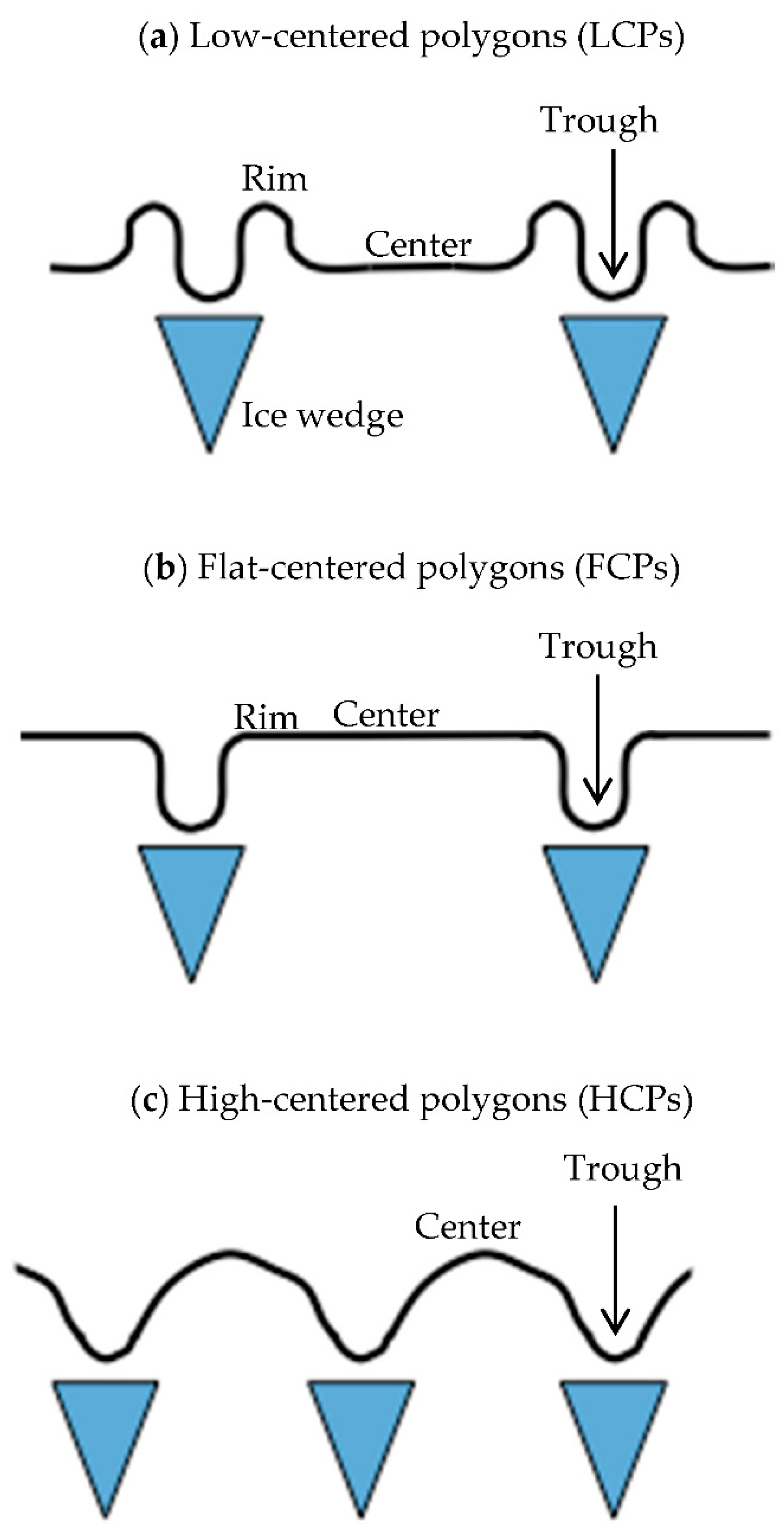
2.1. NGEE-Arctic Site
2.2. Datasets
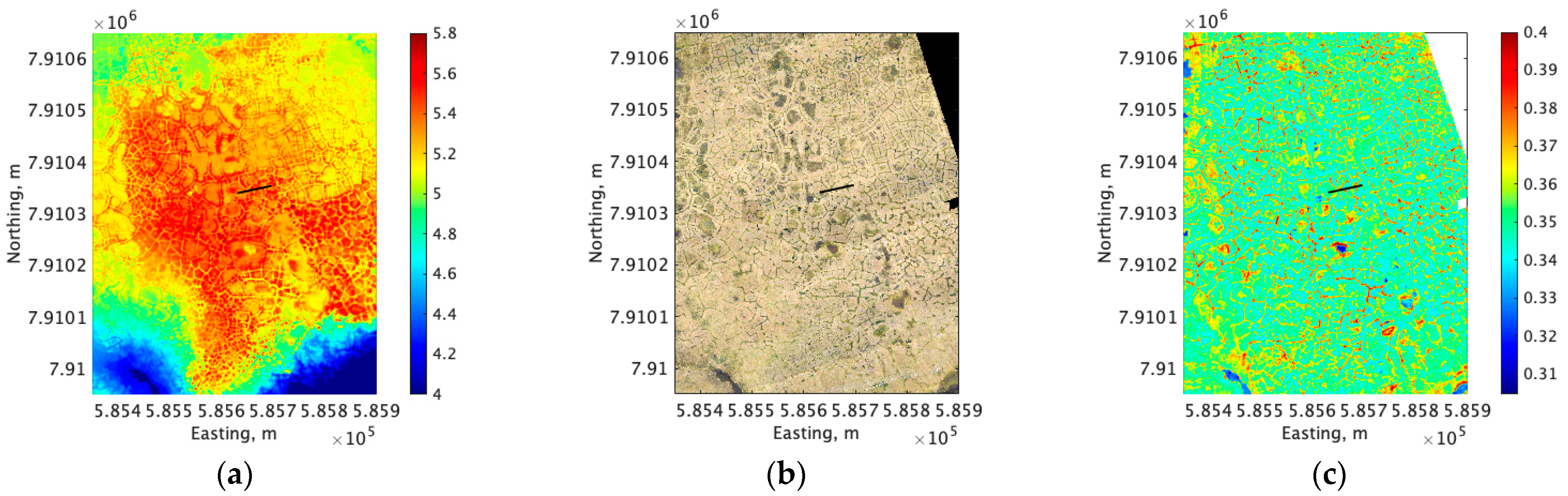
2.2.1. Remote Sensing Data
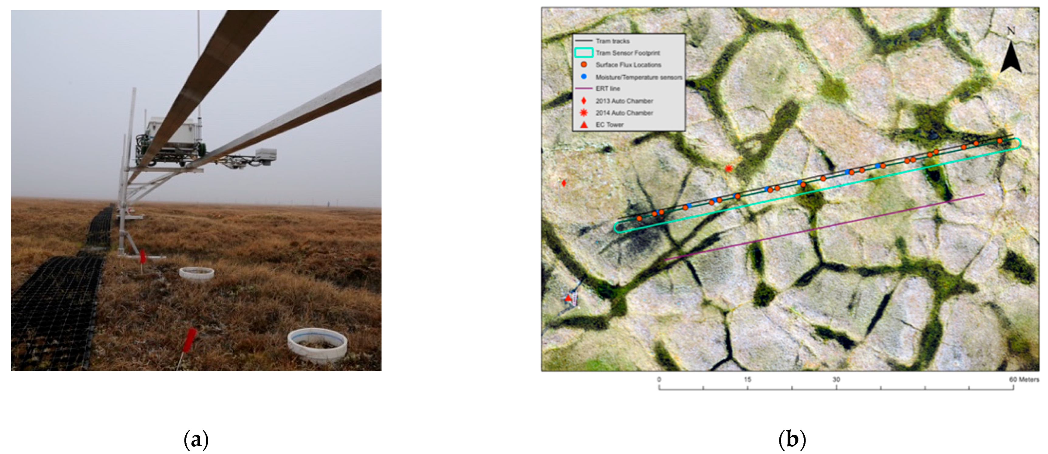
2.2.2. Tram and Flux Datasets
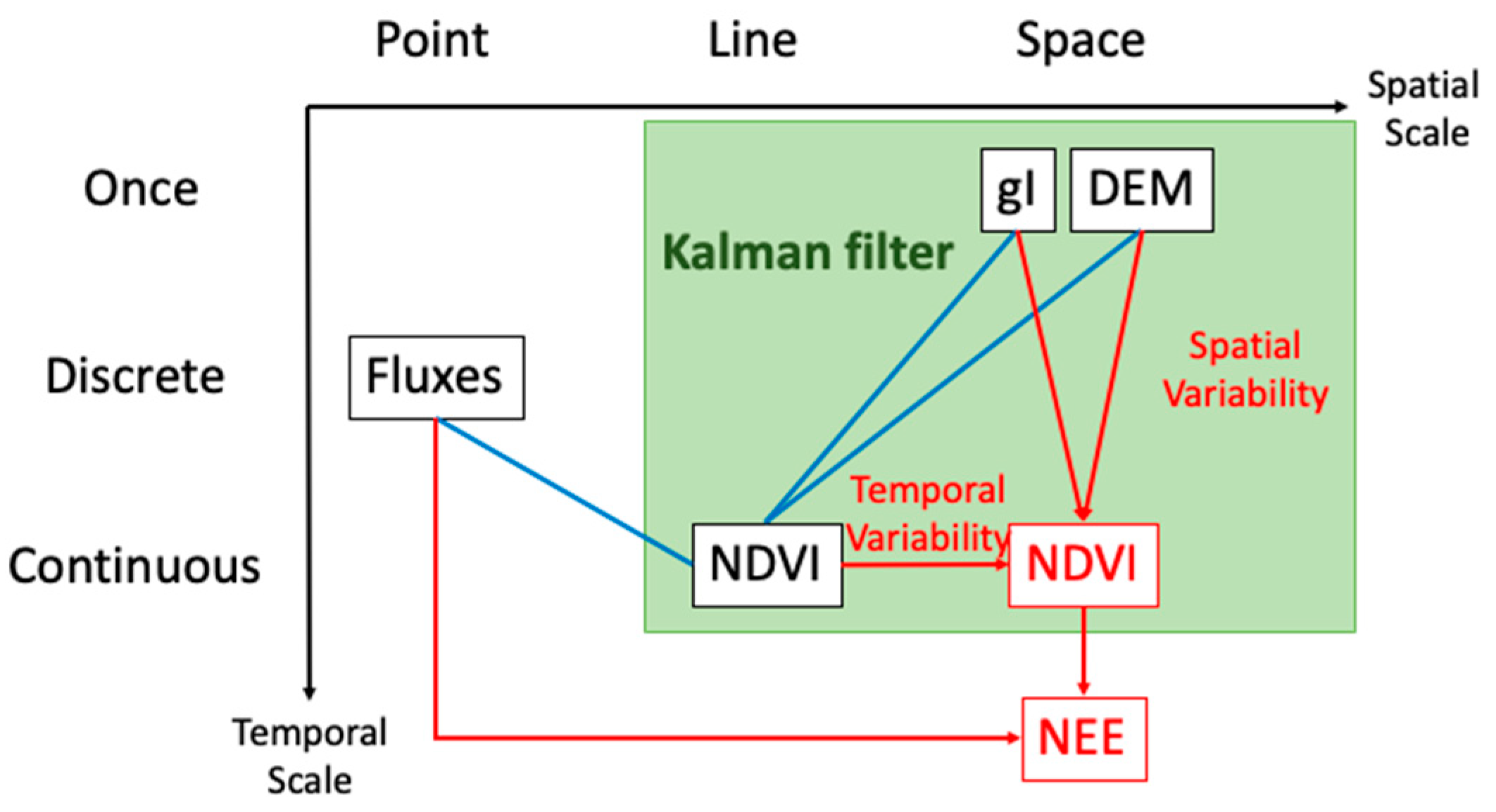
2.3. Integration Strategy
= aV(t), if j-th gI data corresponds to i-th pixel (mT + 1 ≤ j ≤ m).
= bV(t), if j-th gI data corresponds to i-th pixel (mT + 1 ≤ j ≤ m).
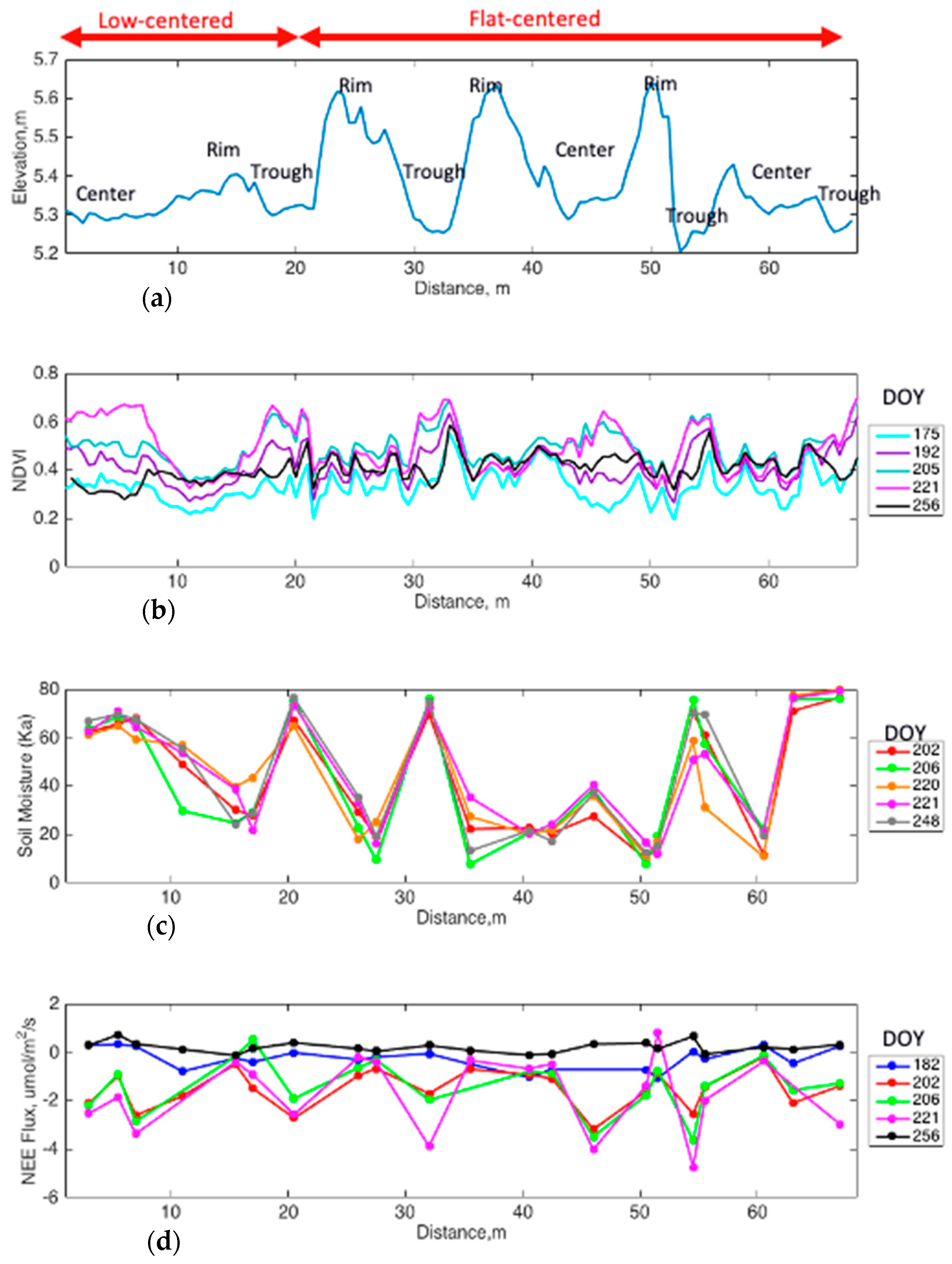
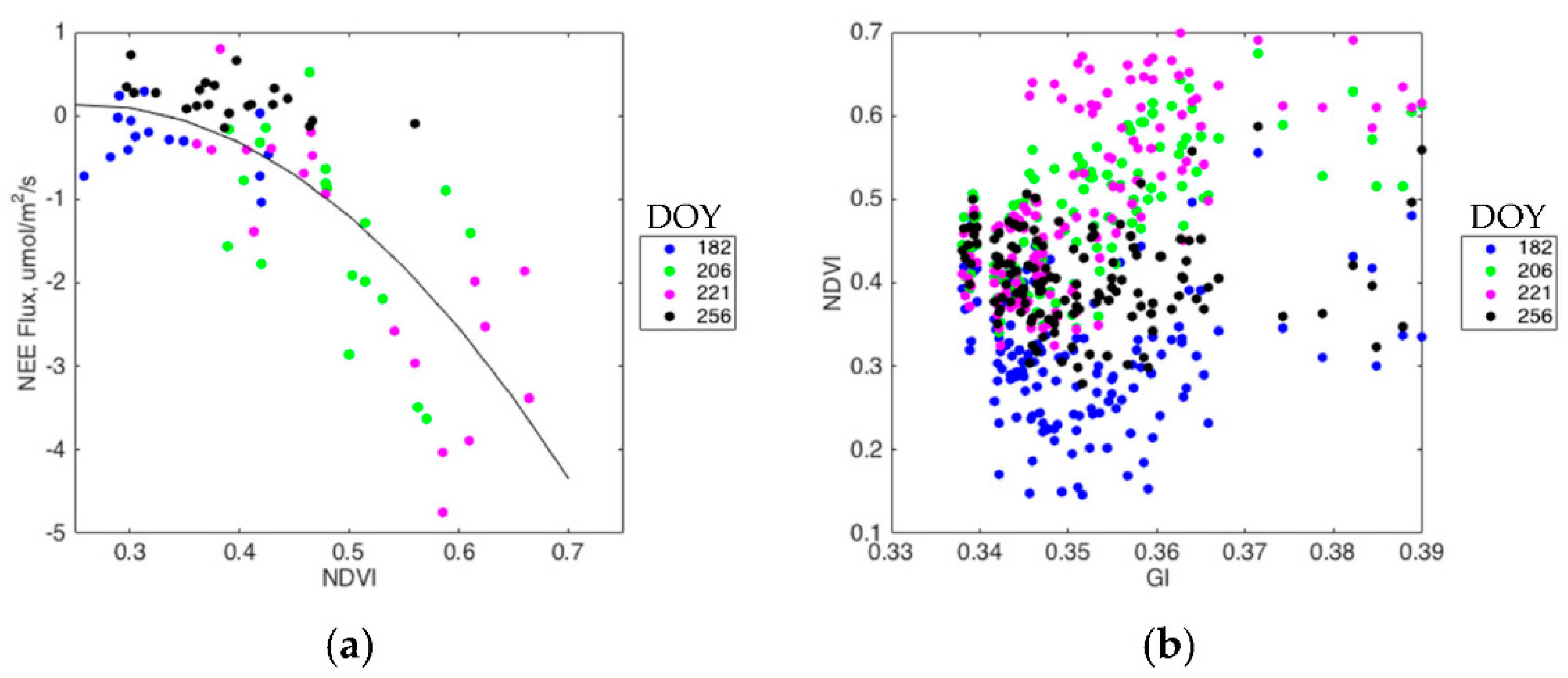
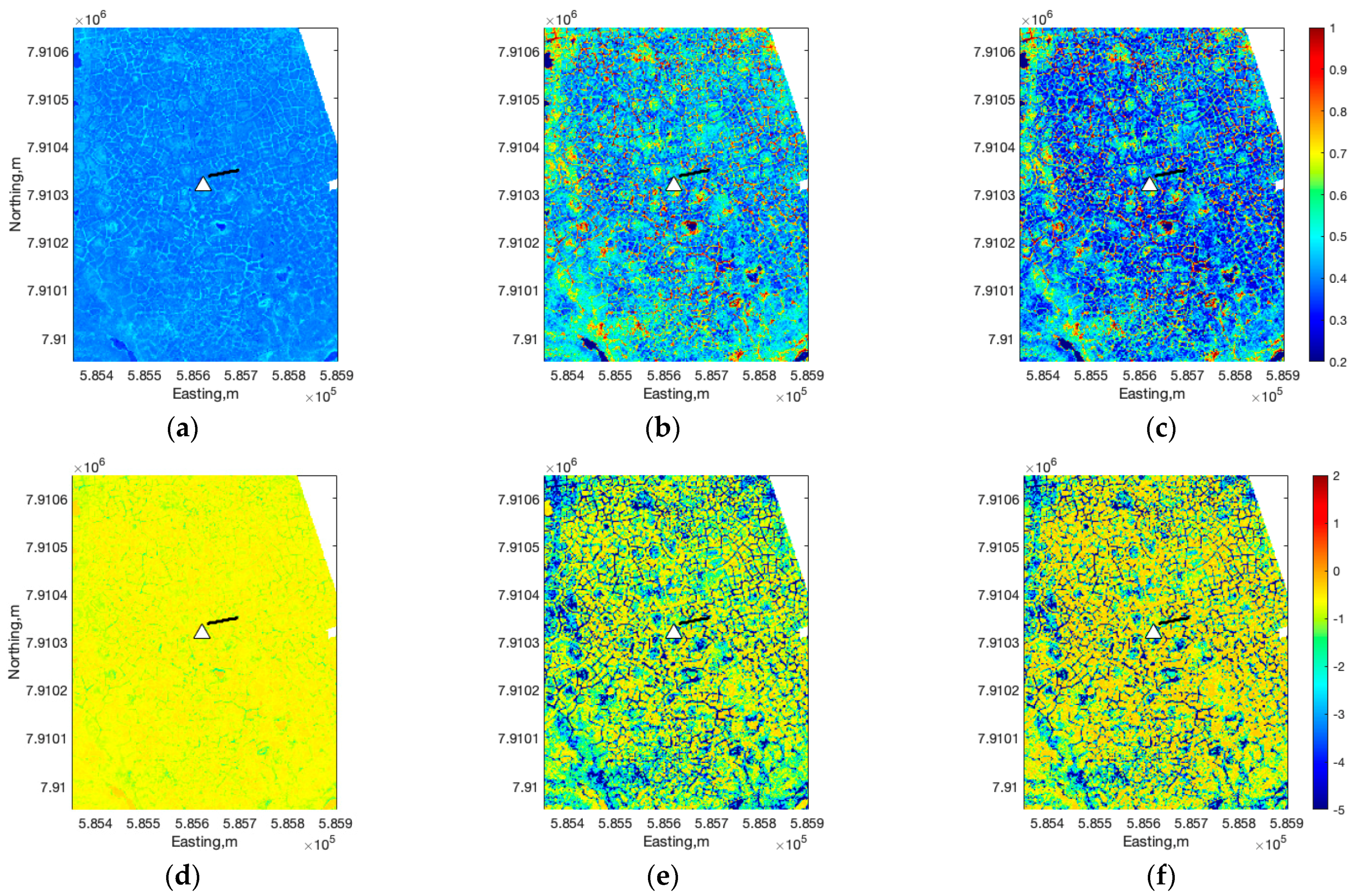
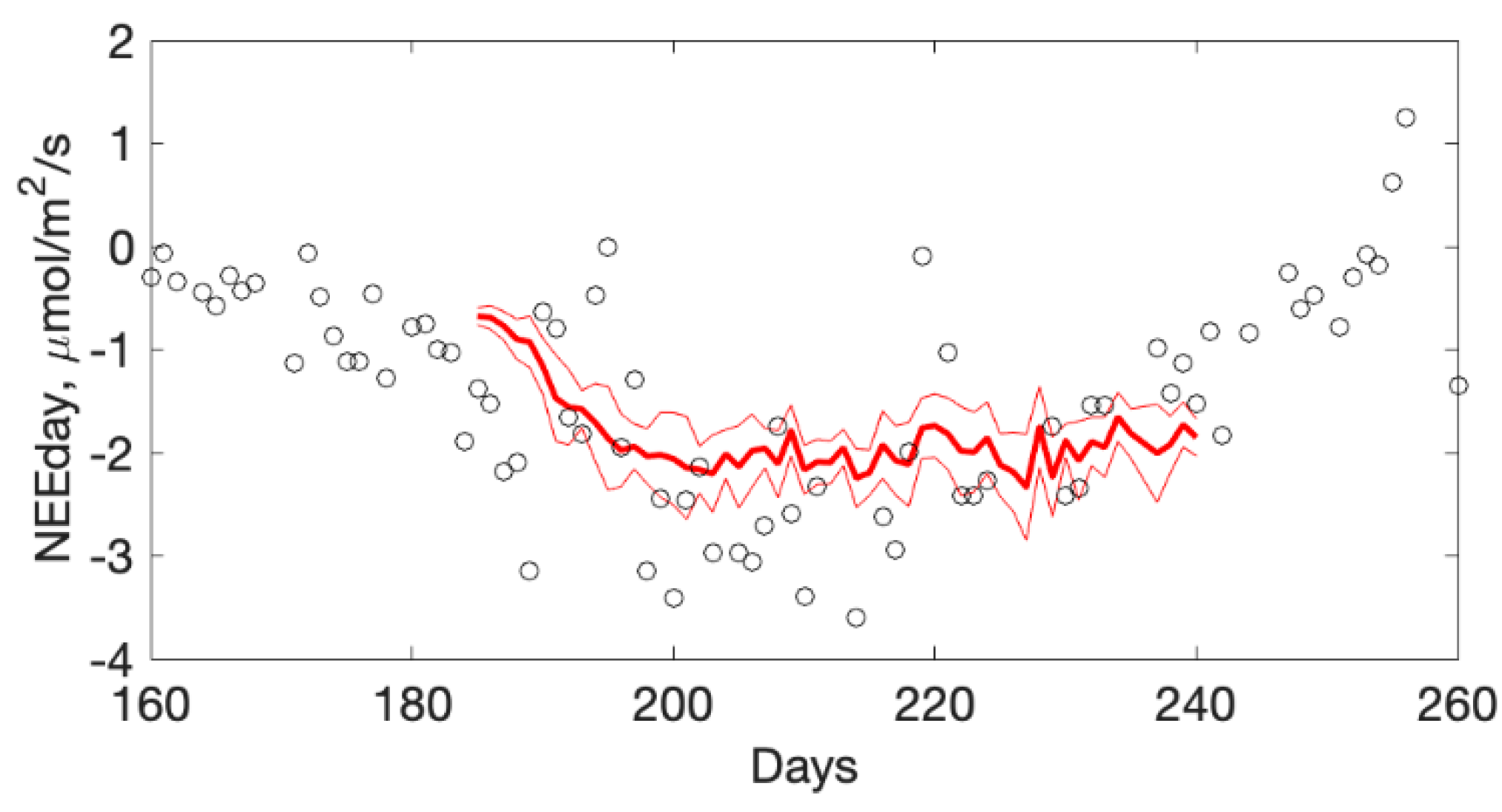
3. Results
4. Discussion
5. Summary
Author Contributions
Funding
Institutional Review Board Statement
Informed Consent Statement
Data Availability Statement
Acknowledgments
Conflicts of Interest
Appendix A
References
- Hinzman, L.D.; Bettez, N.D.; Bolton, W.R.; Chapin, F.S.; Dyurgerov, M.B.; Fastie, C.L.; Griffith, B.; Hollister, R.D.; Hope, A.; Huntington, H.P.; et al. Evidence and implications of recent climate change in northern Alaska and other arctic regions. Clim. Chang. 2005, 72, 251–298. [Google Scholar] [CrossRef]
- Pithan, F.; Mauritsen, T. Arctic amplification dominated by temperature feedbacks in contemporary climate models. Nat. Geosci. 2014, 7, 181–184. [Google Scholar] [CrossRef]
- Kaufman, D.S.; Schneider, D.P.; McKay, N.P.; Ammann, C.M.; Bradley, R.S.; Briffa, K.; Miller, G.H.; Otto-Bliesner, B.L.; Overpeck, J.T.; Vinther, B.; et al. Recent Warming Reverses Long-Term Arctic Cooling. Science 2009, 325, 1236–1239. [Google Scholar] [CrossRef] [PubMed] [Green Version]
- Lawrence, D.M.; Slater, A.G. A projection of severe near-surface permafrost degradation during the 21st century. Geophys. Res. Lett. 2005, 32. [Google Scholar] [CrossRef] [Green Version]
- Zimov, S.A.; Schuur, E.A.G.; Chapin, F.S., III. Climate Change: Permafrost and the Global Carbon Budget. Science 2006, 312, 1612–1613. [Google Scholar] [CrossRef]
- Schuur, E.A.G.; Vogel, J.G.; Crummer, K.G.; Lee, H.; Sickman, J.O.; Osterkamp, T.E. The effect of permafrost thaw on old carbon release and net carbon exchange from tundra. Nat. Cell Biol. 2009, 459, 556–559. [Google Scholar] [CrossRef] [PubMed]
- Forkel, M.; Carvalhais, N.; Rödenbeck, C.; Keeling, R. Enhanced seasonal CO2 exchange caused by amplified plant productivity in northern ecosystems. Science 2016, 351, 696–699. [Google Scholar] [CrossRef] [Green Version]
- Kutzbach, L.; Wagner, D.; Pfeiffer, E.M. Effect of microrelief and vegetation on methane emission from wet polygonal tundra, Lena Delta, Northern Siberia. Biogeochemistry 2004, 69, 341–362. [Google Scholar] [CrossRef] [Green Version]
- Zona, D.; Lipson, D.A.; Zulueta, R.C.; Oberbauer, S.F.; Oechel, W.C. Microtopographic controls on ecosystem functioning in the Arctic Coastal Plain. J. Geophys. Res. Space Phys. 2011, 116, 4. [Google Scholar] [CrossRef] [Green Version]
- Leffingwell, E.D.K. Ground-Ice Wedges: The Dominant Form of Ground-Ice on the North Coast of Alaska. J. Geol. 1915, 23, 635–654. [Google Scholar] [CrossRef]
- Mackay, J.R. Thermally induced movements in ice-wedge polygons, western arctic coast: A long-term study. Géographie Phys. Quat. 2000, 54, 41–68. [Google Scholar] [CrossRef] [Green Version]
- Wainwright, H.M.; Dafflon, B.; Smith, L.J.; Hahn, M.S.; Curtis, J.B.; Wu, Y.; Hubbard, S.S. Identifying mul-tiscale zonation and assessing the relative importance of polygon geomorphology on carbon fluxes in an Arctic tundra ecosystem. J. Geophys. Res. BioGeosci. 2015, 120, 788–808. [Google Scholar] [CrossRef]
- Liljedahl, A.; Boike, J.; Daanen, R.P.; Fedorov, A.; Frost, G.; Grosse, G.; Hinzman, L.D.; Iijima, Y.; Jorgenson, J.C.; Matveyeva, N.; et al. Pan-Arctic ice-wedge degradation in warming permafrost and its influence on tundra hydrology. Nat. Geosci. 2016, 9, 312–318. [Google Scholar] [CrossRef]
- Billings, W.D.; Peterson, K.M. Vegetational Change and Ice-Wedge Polygons through the Thaw-Lake Cycle in Arctic Alaska. Arct. Alp. Res. 1980, 12, 413. [Google Scholar] [CrossRef]
- Kim, Y. Effect of thaw depth on fluxes of CO2 and CH4 in manipulated Arctic coastal tundra of Barrow, Alaska. Sci. Total Environ. 2015, 505, 385–389. [Google Scholar] [CrossRef] [PubMed]
- Knoblauch, C.; Spott, O.; Evgrafova, S.; Kutzbach, L.; Pfeiffer, E. Regulation of methane production, oxidation, and emission by vascular plants and bryophytes in ponds of the northeast Siberian polygonal tundra. J. Geophys. Res. BioGeosci. 2015, 120, 2525–2541. [Google Scholar] [CrossRef]
- Vaughn, L.J.S.; Conrad, M.E.; Bill, M.; Torn, M.S. Isotopic insights into methane production, oxidation, and emissions in Arctic polygon tundra. Glob. Chang. Biol. 2016, 22, 3487–3502. [Google Scholar] [CrossRef] [Green Version]
- Dengel, S.; Torn, M.S. AmeriFlux US-NGB NGEE Arctic Barrow Site. 2020. Available online: https://ameriflux.lbl.gov/sites/siteinfo/US-NGB (accessed on 7 July 2021).
- Arora, B.; Wainwright, H.M.; Dwivedi, D.; Vaughn, L.J.S.; Curtis, J.B.; Torn, M.; Dafflon, B.; Hubbard, S.S. Evaluating temporal controls on greenhouse gas (GHG) fluxes in an Arctic tundra environment: An entropy-based approach. Sci. Total. Environ. 2019, 649, 284–299. [Google Scholar] [CrossRef] [PubMed] [Green Version]
- Eckhardt, T.; Knoblauch, C.; Kutzbach, L.; Holl, D.; Simpson, G.; Abakumov, E.; Pfeiffer, E.-M. Partitioning net ecosystem exchange of CO2 on the pedon scale in the Lena River Delta, Siberia. Biogeosciences 2019, 16, 1543–1562. [Google Scholar] [CrossRef] [Green Version]
- Sturtevant, C.S.; Oechel, W. Spatial variation in landscape-level CO2 and CH4 fluxes from arctic coastal tundra: Influence from vegetation, wetness, and the thaw lake cycle. Glob. Chang. Biol. 2013, 19, 2853–2866. [Google Scholar] [CrossRef]
- Zulueta, R.C.; Oechel, W.; Loescher, H.W.; Lawrence, W.T.; Paw, K.T. Aircraft-derived regional scale CO2 fluxes from vegetated drained thaw-lake basins and interstitial tundra on the Arctic Coastal Plain of Alaska. Glob. Chang. Biol. 2011, 17, 2781–2802. [Google Scholar] [CrossRef]
- Hubbard, S.S.; Gangodagamage, C.; Dafflon, B.; Wainwright, H.; Peterson, J.; Gusmeroli, A.; Tweedie, C. Quantifying and relating land-surface and subsurface variability in permafrost environments using LiDAR and surface geophysical datasets. Hydrogeol. J. 2013, 21, 149–169. [Google Scholar] [CrossRef]
- Dafflon, B.; Hubbard, S.; Ulrich, C.; Peterson, J.; Wu, Y.; Wainwright, H.; Kneafsey, T.J. Geophysical estimation of shallow permafrost distribution and properties in an ice-wedge polygon-dominated Arctic tundra region. Geophysics 2016, 81, WA247–WA263. [Google Scholar] [CrossRef]
- Andresen, C.G.; Lougheed, V.L. Disappearing Arctic tundra ponds: Fine-scale analysis of surface hydrology in drained thaw lake basins over a 65 year period (1948–2013). J. Geophys. Res. BioGeosci. 2015, 120, 466–479. [Google Scholar] [CrossRef]
- Dafflon, B.; Oktem, R.; Peterson, J.; Ulrich, C.; Tran, A.P.; Romanovsky, V.; Hubbard, S.S. Coincident aboveground and belowground autonomous monitoring to quantify covariability in permafrost, soil, and vegetation properties in Arctic tundra. J. Geophys. Res. BioGeosci. 2017, 122, 1321–1342. [Google Scholar] [CrossRef] [Green Version]
- McMichael, C.E. Estimating CO2 exchange at two sites in Arctic tundra ecosystems during the growing season using a spectral vegetation index. Int. J. Remote Sens. 1999, 20, 683–698. [Google Scholar] [CrossRef]
- Johnson, T.J.; Versteeg, R.; Thomle, J.; Hammond, G.; Chen, X.; Zachara, J.M. Four-dimensional electrical conductivity monitoring of stage-driven river water intrusion: Accounting for water table effects using a transient mesh boundary and conditional inversion constraints. Water Resour. Res. 2015, 51, 6177–6196. [Google Scholar] [CrossRef]
- Baldocchi, D.; Falge, E.; Gu, L.; Olson, R.; Hollinger, D.; Running, S.; Fuentes, J. Fluxnet: A new tool to study the temporal and spatial variability of ecosystem-scale carbon dioxide, water vapor, and energy flux densities. Bull. Am. Meteorol. Soc. 2001, 82, 2415–2434. [Google Scholar] [CrossRef]
- Baldocchi, D.D. Assessing the eddy covariance technique for evaluating carbon dioxide exchange rates of ecosystems: Past, present and future. Glob. Chang. Biol. 2003, 9, 479–492. [Google Scholar] [CrossRef] [Green Version]
- Healey, N.C.; Oberbauer, S.F.; Ahrends, H.E.; Dierick, D.; Welker, J.M.; Leffler, A.J.; Tweedie, C.E. A Mobile Instrumented Sensor Platform for Long-Term Terrestrial Ecosystem Analysis: An Example Application in an Arctic Tundra Ecosystem. J. Environ. Inform. 2014, 24, 1–10. [Google Scholar] [CrossRef]
- Wainwright, H.M.; Chen, J.; Sassen, D.S.; Hubbard, S.S. Bayesian hierarchical approach and geophysical data sets for estimation of reactive facies over plume scales. Water Resour. Res. 2014, 50, 4564–4584. [Google Scholar] [CrossRef]
- Wainwright, H.M.; Seki, A.; Chen, J.; Saito, K. A multiscale Bayesian data integration approach for mapping air dose rates around the Fukushima Daiichi Nuclear Power Plant. J. Environ. Radioact. 2017, 167, 62–69. [Google Scholar] [CrossRef] [Green Version]
- Wainwright, H.M.; Liljedahl, A.K.; Dafflon, B.; Ulrich, C.; Peterson, J.E.; Gusmeroli, A.; Hubbard, S.S. Mapping snow depth within a tundra ecosystem using multiscale observations and Bayesian methods. Cryosphere 2017, 11, 857–875. [Google Scholar] [CrossRef] [Green Version]
- Wikle, C.K.; Milliff, R.F.; Nychka, D.; Berliner, L.M. Spatiotemporal hierarchical Bayesian modeling: Tropical ocean surface winds. J. Am. Stat. Assoc. 2001, 96, 382–397. [Google Scholar] [CrossRef] [Green Version]
- Chen, J.; Hubbard, S.S.; Williams, K.H. Data-driven approach to identify field-scale biogeochemical transitions using geochemical and geophysical data and hidden Markov models: Development and application at a uranium-contaminated aquifer. Water Resour. Res. 2013, 49, 6412–6424. [Google Scholar] [CrossRef]
- Fox, A.M.; Huntley, B.; Lloyd, C.R.; Williams, M.; Baxter, R. Net ecosystem exchange over heterogeneous Arctic tundra: Scaling between chamber and eddy covariance measurements. Glob. Biogeochem. Cycles 2008, 22. [Google Scholar] [CrossRef]
- Fox, A.; Williams, M.; Richardson, A.D.; REFLEX Team. The Reflex project: Comparing different algorithms and implementations for the inversion of a terrestrial ecosystem model against eddy covariance data. Agric. For. Meteorol. 2009, 149, 1597–1615. [Google Scholar] [CrossRef] [Green Version]
- Williams, M.; Richardson, A.D.; Reichstein, M.; Stoy, P.C.; Peylin, P.; Verbeeck, H.; Carvalhais, N.; Jung, M.; Hollinger, D.Y.; Kattge, J.; et al. Improving land surface models with FLUXNET data. Biogeosciences 2009, 6, 1341–1359. [Google Scholar] [CrossRef] [Green Version]
- Sachs, T.; Giebels, M.; Boike, J.; Kutzbach, L. Environmental controls on CH4 emission from polygonal tundra on the microsite scale in the Lena river delta, Siberia. Glob. Chang. Biol. 2010, 16, 3096–3110. [Google Scholar] [CrossRef]
- Zhang, Y.; Sachs, T.; Li, C.; Boike, J. Upscaling methane fluxes from closed chambers to eddy covariance based on a permafrost biogeochemistry integrated model. Glob. Chang. Biol. 2011, 18, 1428–1440. [Google Scholar] [CrossRef] [Green Version]
- Sahoo, A.K.; De Lannoy, G.J.; Reichle, R.; Houser, P. Assimilation and downscaling of satellite observed soil moisture over the Little River Experimental Watershed in Georgia, USA. Adv. Water Resour. 2013, 52, 19–33. [Google Scholar] [CrossRef]
- Schmidt, F.; Wainwright, H.M.; Faybishenko, B.; Denham, M.; Eddy-Dilek, C. In Situ Monitoring of Groundwater Contamination Using the Kalman Filter. Environ. Sci. Technol. 2018, 52, 7418–7425. [Google Scholar] [CrossRef] [Green Version]
- Engstrom, R.; Hope, A.; Kwon, H.; Stow, D. The Relationship between Soil Moisture and NDVI Near Barrow, Alaska. Phys. Geogr. 2008, 29, 38–53. [Google Scholar] [CrossRef]
- Kanevskiy, M.; Shur, Y.; Jorgenson, T.; Brown, D.R.; Moskalenko, N.; Brown, J.; Walker, D.A.; Raynolds, M.K.; Buchhorn, M. Degradation and stabilization of ice wedges: Implications for assessing risk of thermokarst in northern Alaska. Geomorphology 2017, 297, 20–42. [Google Scholar] [CrossRef]
- Lin, D.H.; Johnson, D.R.; Andresen, C.; Tweedie, C.E. 2012 High spatial resolution decade-time scale land cover change at multiple locations in the Beringian Arctic (1948–2000s). Environ. Res. Lett. 2012, 7, 025502. [Google Scholar] [CrossRef] [Green Version]
- Hinkel, K.M.; Eisner, W.R.; Bockheim, J.G.; Nelson, F.E.; Peterson, K.M.; Dai, X. Institute of Arctic and Alpine Research (INSTAAR) University of Colorado Spatial Extent, Age, and Carbon Stocks in Drained Thaw Lake Basins on the Barrow Peninsula, Alaska. Arct. Antarct. Alp. Res. 2003, 35, 291–300. [Google Scholar] [CrossRef] [Green Version]
- Langford, Z.; Kumar, J.; Hoffman, F.M.; Norby, R.J.; Wullschleger, S.D.; Sloan, V.L.; Iversen, C.M. Mapping Arctic Plant Functional Type Distributions in the Barrow Environmental Observatory Using WorldView-2 and LiDAR Datasets. Remote Sens. 2016, 8, 733. [Google Scholar] [CrossRef] [Green Version]
- Torn, M.; Dafflon, B.; Dengel, S.; Curtis, B.; Chafe, O.; Moyes, A.; Serbin, S.; Lewin, K.; Breen, A.; Velliquette, T.; et al. NGEE Arctic Tram: Overview of Tram-Mounted Instruments, Co-Located Data, Measurement Position, Elevation and Polygon Characterization, Barrow, Alaska, 2014–2018. 2019. Available online: https://ngee-arctic.ornl.gov/data/pages/NGA177.html (accessed on 8 July 2021). [CrossRef]
- Kormann, R.; Meixner, F.X. An Analytical Footprint Model for Non-Neutral Stratification. Bound. Layer Meteorol. 2001, 99, 207–224. [Google Scholar] [CrossRef]
- Wainwright, M.J.; Jordan, M.I. Graphical Models, Exponential Families, and Variational Inference. Found. Trends Mach. Learn. 2007, 1, 1–305. [Google Scholar] [CrossRef] [Green Version]
- La Puma, I.P.; Philippi, T.E.; Oberbauer, S.F. Relating NDVI to ecosystem CO2 exchange patterns in response to season length and soil warming manipulations in arctic Alaska. Remote Sens. Environ. 2007, 109, 225–236. [Google Scholar] [CrossRef]
- Loranty, M.M.; Goetz, S.; Rastetter, E.; Rocha, A.V.; Shaver, G.R.; Humphreys, E.; Lafleur, P.M. Scaling an Instantaneous Model of Tundra NEE to the Arctic Landscape. Ecol. Appl. 2011, 14, 76–93. [Google Scholar] [CrossRef]
- Toomey, M.; Friedl, M.A.; Frolking, S.; Hufkens, K.; Klosterman, S.; Sonnentag, O.; Baldocchi, D.D.; Bernacchi, C.; Biraud, S.C.; Bohrer, G.; et al. Greenness indices from digital cameras predict the timing and seasonal dynamics of canopyscale photosynthesis. Ecol. Appl. 2015, 25, 99–115. [Google Scholar] [CrossRef] [Green Version]
- Hamilton, J.D. Time Series Analysis; Princeton University Press: Princeton, NJ, USA, 1994; Volume 2. [Google Scholar]
- Rastetter, E.B.; Williams, M.; Griffin, K.L.; Kwiatkowski, B.L.; Tomasky, G.; Potosnak, M.J.; Stoy, P.C.; Shaver, G.R.; Stieglitz, M.; Hobbie, J.E.; et al. Processing Arctic Eddy-Flux Data Using a Simple Carbon-Exchange Model Embedded in the Ensemble Kalman Filter. Ecol. Appl. 2010, 20, 1285–1301. [Google Scholar] [CrossRef] [PubMed] [Green Version]
- Beck, P.S.; Goetz, S.J. Corrigendum: Satellite observations of high northern latitude vegetation productivity changes between 1982 and 2008: Ecological variability and regional differences. Environ. Res. Lett. 2012, 7, 029501. [Google Scholar] [CrossRef] [Green Version]
- Rubin, Y. Applied Stochastic Hydrogeology; Oxford University Press (OUP): Oxford, UK, 2003. [Google Scholar]
- Lara, M.J.; McGuire, A.D.; Euskirchen, E.S.; Tweedie, C.E.; Hinkel, K.M.; Skurikhin, A.N.; Romanovsky, V.E.; Grosse, G.; Bolton, W.R.; Genet, H. Polygonal tundra geomorphological change in response to warming alters future CO2 and CH4 flux on the Barrow Peninsula. Glob. Chang. Biol. 2015, 21, 1634–1651. [Google Scholar] [CrossRef]
- Bickel, P.J.; Hammel, E.A.; O’Connell, J.W. Sex Bias in Graduate Admissions: Data from Berkeley. Science 1975, 187, 398–404. [Google Scholar] [CrossRef] [Green Version]


| Av. NDVI | (SD) | Av. NEEday, μmol/m2/s | (SD) | Spatial Coverage | ||
|---|---|---|---|---|---|---|
| LCP | Trough | 0.59 | (0.014) | −3.4 | (0.64) | 0.14 |
| Center | 0.52 | (0.010) | −2.1 | (0.41) | 0.36 | |
| Rim | 0.44 | (0.011) | −1.4 | (0.34) | 0.5 | |
| FCP | Trough | 0.58 | (0.016) | −3.2 | (0.63) | 0.29 |
| Center | 0.48 | (0.016) | −1.7 | (0.37) | 0.21 | |
| Rim | 0.41 | (0.016) | −1.1 | (0.27) | 0.5 | |
| HCP | Trough | 0.56 | (0.013) | −2.8 | (0.56) | 0.5 |
| Center | 0.43 | (0.012) | −1.2 | (0.30) | 0.5 |
| Av. NDVI | (SD) | Av. NEEday, μmol/m2/s | (SD) | |
|---|---|---|---|---|
| LCP | 0.49 | (0.011) | −2.4 | (0.42) |
| FCP | 0.48 | (0.016) | −2.3 | (0.43) |
| HCP | 0.50 | (0.012) | −2.6 | (0.45) |
Publisher’s Note: MDPI stays neutral with regard to jurisdictional claims in published maps and institutional affiliations. |
© 2021 by the authors. Licensee MDPI, Basel, Switzerland. This article is an open access article distributed under the terms and conditions of the Creative Commons Attribution (CC BY) license (https://creativecommons.org/licenses/by/4.0/).
Share and Cite
Wainwright, H.M.; Oktem, R.; Dafflon, B.; Dengel, S.; Curtis, J.B.; Torn, M.S.; Cherry, J.; Hubbard, S.S. High-Resolution Spatio-Temporal Estimation of Net Ecosystem Exchange in Ice-Wedge Polygon Tundra Using In Situ Sensors and Remote Sensing Data. Land 2021, 10, 722. https://doi.org/10.3390/land10070722
Wainwright HM, Oktem R, Dafflon B, Dengel S, Curtis JB, Torn MS, Cherry J, Hubbard SS. High-Resolution Spatio-Temporal Estimation of Net Ecosystem Exchange in Ice-Wedge Polygon Tundra Using In Situ Sensors and Remote Sensing Data. Land. 2021; 10(7):722. https://doi.org/10.3390/land10070722
Chicago/Turabian StyleWainwright, Haruko M., Rusen Oktem, Baptiste Dafflon, Sigrid Dengel, John B. Curtis, Margaret S. Torn, Jessica Cherry, and Susan S. Hubbard. 2021. "High-Resolution Spatio-Temporal Estimation of Net Ecosystem Exchange in Ice-Wedge Polygon Tundra Using In Situ Sensors and Remote Sensing Data" Land 10, no. 7: 722. https://doi.org/10.3390/land10070722
APA StyleWainwright, H. M., Oktem, R., Dafflon, B., Dengel, S., Curtis, J. B., Torn, M. S., Cherry, J., & Hubbard, S. S. (2021). High-Resolution Spatio-Temporal Estimation of Net Ecosystem Exchange in Ice-Wedge Polygon Tundra Using In Situ Sensors and Remote Sensing Data. Land, 10(7), 722. https://doi.org/10.3390/land10070722