Article

Do ARMA Models Provide Better Gap Filling in Time Series of Soil Temperature and Soil Moisture? The Case of Arable Land in the Kulunda Steppe, Russia

1
Department of Theoretical Cybernetics and Applied Mathematics, Faculty of Mathematics and Information Technologies, Altai State University, 656049 Barnaul, Russia
2
Institute of Geosciences and Geography, Martin Luther University Halle-Wittenberg, 06108 Halle, Germany
*
Author to whom correspondence should be addressed.
Land 2021, 10(6), 579; https://doi.org/10.3390/land10060579
Submission received: 17 January 2021 / Revised: 9 May 2021 / Accepted: 17 May 2021 / Published: 31 May 2021

Abstract

:
The adoption of climate-smart agriculture requires the comprehensive development of environmental monitoring tools, including online observation of climate and soil settings. They are often designed to measure soil properties automatically at different depths at hour or minute intervals. It is essential to have a complete dataset to use statistical models for the prediction of soil properties and to make short-term decisions regarding soil tillage operations and irrigation during a vegetation period. This is also important in applied hydrological studies. Nevertheless, the time series of soil hydrological measurements often have data gaps for different reasons. The study focused on solving a problem of gap-filling in hourly time series of soil temperature and moisture, measured at the 30 cm depth using a weighted gravitation lysimeter station while meteorological data were recorded simultaneously by a weather station. The equipment was installed in the Kulunda Steppe in the Altai Krai, Russia. Considering that climate conditions affect soil temperature and moisture content directly, we did a comparative analysis of the gap-filling performance using the three imputation methods—linear interpolation, multiple linear regression, and extended ARMA (p,q) models with exogenous climatic variables. The results showed that, according to the minimum of the mean absolute error, ARMA (p,q) models with optimally selected order parameters, and an adaptive window, had some advantages compared to other single-imputation methods. The ARMA (p,q) model produced a good quality of gap-filling in time series with the mean absolute error of 0.19 °C and 0.08 Vol. % for soil temperature and moisture content, respectively. The findings supplemented the methodology of hydrological data processing and the development of digital tools for the online monitoring of climate and soil properties in agriculture.

1. Introduction

The monitoring of soil temperature and moisture at different depths is vital in agriculture to plan seasonal soil tillage operations, soil water conservation, and evaluation of crop growing conditions. Extreme soil temperature and low soil moisture negatively affect crop growth [1]. These soil properties significantly influence crop yield [2,3,4] and can cause physical damage and yield loss. Moreover, the findings within interdisciplinary studies [5] confirmed that the amount of moisture in the soil is linearly related to microbial respiration and affects their interaction. The data on soil temperature and soil moisture help in estimating the soil heat flux, which can provide data for the analysis of water balance and actual evapotranspiration (ETa) [6,7,8], with water content being the primary indicator to assess crop water stress [6,9,10]. Finally, soil temperature and moisture monitoring are critical because climate data do not provide complete information about soil properties affecting plant growth.
Modern agricultural management, including the concepts of digital agriculture and climate-smart agriculture, requires the development of applied digital tools for the online monitoring of various soil indicators at all stages of a growing season. The continuous field monitoring of soil properties, such as soil temperature and moisture content, is important in arid and semi-arid areas where lack of crop water is more frequent. The Kulunda Steppe belongs to the semi-arid climatic zone located in southwestern Siberia. The study focuses on the part of the Kulunda Steppe within the Altai Krai, a Russian region. This territory plays an essential role in regional grain and sunflower production [11]. Lack of soil moisture is the main limiting factor for crop yield [3]. Thus, optimizing the soil water regime can solve several topical problems in agriculture. The soil cover consists of chestnut soils, meadow-chestnut soils, meadow soils, solonetz, and solonchaks [8], where soil textures are different. Sandy loams are predominant (15–19% clay, 11–20% silt, 65–70% sand). The humus and carbon contents are comparatively high and vary from 2 to 8% [12]. The current climate trends showed future aridization that requires the adaptation of farming systems in the region. Thereby, in the context of introducing drought-resistant farming practices, the modern climate–soil monitoring network was installed in 2013 as a part of the international Russian–German project [13]. The equipment was configured to measure climatic and soil hydrological properties every hour in an online regime.
As standard practice shows, the time series of field monitoring often have data gaps for many reasons (systematic errors, human reasons (agricultural machinery movements, power outages, etc.), and equipment failures). Different climate seasonal events such as spring water flow or high wind speed, lead to gaps, outliers, and noise in the lysimeter measurements [14,15]. However, most approaches in hydrological analysis demand complete time series, and using data with missing values usually decreases the power of applied statistical models and increases uncertainty. Besides, introducing modern water management practices together with local online monitoring of soil hydrological settings at topsoil gives farmers vital information about the water stress of plants to make decisions regarding irrigation and soil tillage operations. Obviously, when we have data gaps in soil hydrological measurements, especially those that are longer than 24 h, such decision making becomes more difficult, and online monitoring tools lose their effectiveness. Therefore, to decrease uncertainty and understand better plant growing conditions in the area under study, as well as to apply various hydrological methods and statistical models, we can reconstruct the missing data in soil hydrological measurements. Finally, we can both estimate missing values and predict soil settings based on statistical models.
There are many methods of gap-filling in time series determined by the nature of the process. Especially in studies that produce a large amount of data, such as gas exchange or energy flow measurements, such techniques are often mandatory [16,17]. The data of soil hydrological properties such as soil temperature, soil moisture content, and climate time series often follow stable non-linear trends with seasonality over time [18,19]. For these reasons, in previous studies, gap filling was often based on harmonic analysis [20,21], polynomial interpolation, and non-linear approximation [22,23]. The cross-sectional nature of climate and soil-hydrological measurements and high autocorrelation provides an application of various statistical approaches. For estimating soil temperature based on observed air temperature [24], combining principal component analysis (PCA), linear regression models [25,26], and autoregression moving average models in annual and daily rainfall prediction [27] were used. Developments in data science brought a new wave of methods and their uttermost applications in missing data-handling techniques. The neural networks [19], polynomial models with adaptive windows [14,15], and machine learning methods and algorithms became used more often. In several studies [14,15,28], the polynomial approximation methods with an adaptive window (AWAT filter routine) were used to solve two problems of lysimeter data processing. The first problem was to filter hydrological data from noise. The second task was to estimate missing values in short-term gaps. However, other studies [28,29] prefer simple linear interpolation or single-imputation techniques, using mean or median values to fill short-term gaps (<5 h). What quality of gap-filling, based on such a convenient approach, do we receive? What is the share of lost information that could have been recovered by using more sophisticated methods? According to Y. Gao, C. Merz, G. Lischeid, and M. Schneider [18], families of adaptive statistical models—ARIMA (an autoregressive integrated moving average) model and ARCH (autoregressive conditional heteroscedasticity) model—are the most suitable for the nature of hydrological data. The application of these methods depends on the stationary of the original stochastic process. Based on this expert knowledge, the main research question was—What level of performance of the ARIMA models do we have in gap-filling in hourly time series of the soil temperature and soil moisture of topsoil, taking into account climatic settings? Despite a wealth of studies in soil hydrology, there is a shortage of studies that focused on the comparative analysis of methods performance to estimate missing values in hourly time series of soil temperature and soil moisture, measured by a weighable gravitational lysimeter station at topsoil.
The study objectivities are (1) to test extended ARIMA models with exogenous climate variables as statistical tools for gap filling in hourly time series of soil temperature and soil moisture at topsoil, (2) to compare the accuracy of missing values recovering based on three methods (linear interpolation, multiple linear regression and extended ARIMA model), and (3) to make recommendations regarding gap-filling techniques depending on the duration of a data gap.

2. Materials and Methods

2.1. The Monitoring Network

The network for monitoring climatic and soil hydrological settings was established in the dry steppe of the Kulunda Plain. This network was installed on the private farm “Partner” located in the village of Poluyamki in the Mikhaylovsky district in the Altai Krai. The installation was undertaken in the period 2012–2013 as a part of the Kulunda Project [30]. A weather station (WS) was installed, manufactured by German company “ecoTech” and a weighable gravitation lysimeter station (LYS) was also built, manufactured by “UGT-Muencheberg” (Germany). The equipment design and its parameters were already described in detail in several papers [8,12,28]. Two soil monoliths were extracted from a cultivated field (Monolith 1) and grassland (Monolith 2) separately to install LYS. The grassland had not been cultivated since 1950, while the arable land was cultivated according to the conventional tillage practice. Each monolith had a 1 m square of surface area and 2 m depth. According to FAO guidelines [28], the soils in monoliths belonged to Calcic Chernozems. The time of data registration was synchronized at both stations.
The equipment configuration allowed for sending data online through a regional mobile communication network and storing them in a data server at the digital platform of the Altai State University. The monitoring network continuously recorders the climate and soil properties in the studied area. This allows us to analyze and predict crop growing conditions in a short-term period. Additionally, we can detect the crop water stress and days of droughts, analyze water balance and actual evapotranspiration.
The equipment continuously measured climatic and soil hydrological indicators in a minute interval and automatically computed them to hourly data. The WS measured the following meteorological data—air temperature (°C), air humidity (%), atmospheric pressure (hPa), solar radiation (W/m2), wind speed (m/sec), wind direction (decimal degree), and precipitation (mm). The lysimeter measured temperature (°C), moisture (Vol. %), and water retention (hPa) at three different depths of soil (30, 50, and 120 cm).

2.2. Available Data and Description

We focused on soil temperature and moisture content data, measured by the lysimeter station at 30 cm in the arable land (Monolith 1) and natural steppe vegetation (Monolith 2). The most critical period for recovering the lost data is the crop growing season, which usually starts in May and ends in September in the studied area. To analyze the performance of different gap-filling routines, a sample of artificial data gaps of various durations from short (1–12 h) and middle (13–24 h) to long (25–50 h) had to be investigated. It demanded a complete time series of meteorological and lysimeter measurements. We obtained a complete hourly time series of climate data for the whole period (2013–2019). The lysimeter data had some considerable gaps, which significantly limited the available data for our analysis. We used the entire time series from August to September in 2013, June 2014, from May to September in 2015 and 2016, and from May to August in 2017, 2018, and 2019. Thus, the test period covered different seasons of crop growing and climatic conditions.
In general, data preparation techniques for WS and LYS were similar. First, we converted hourly cumulative data of precipitation measured through multisensory “Vaisala” (WS) to absolute values per hour. Second, all data during system error or noticeable outliers were removed. Finally, we shaped a cross-sectional dataset consisting of the complete hourly time series of meteorological and lysimeter data (soil temperature and moisture content) for the vegetation periods of 2013–2019 (14,288 observations, in total for each monolith). The climate conditions and features of soil measurements at 30 cm are summarized in Appendix A.
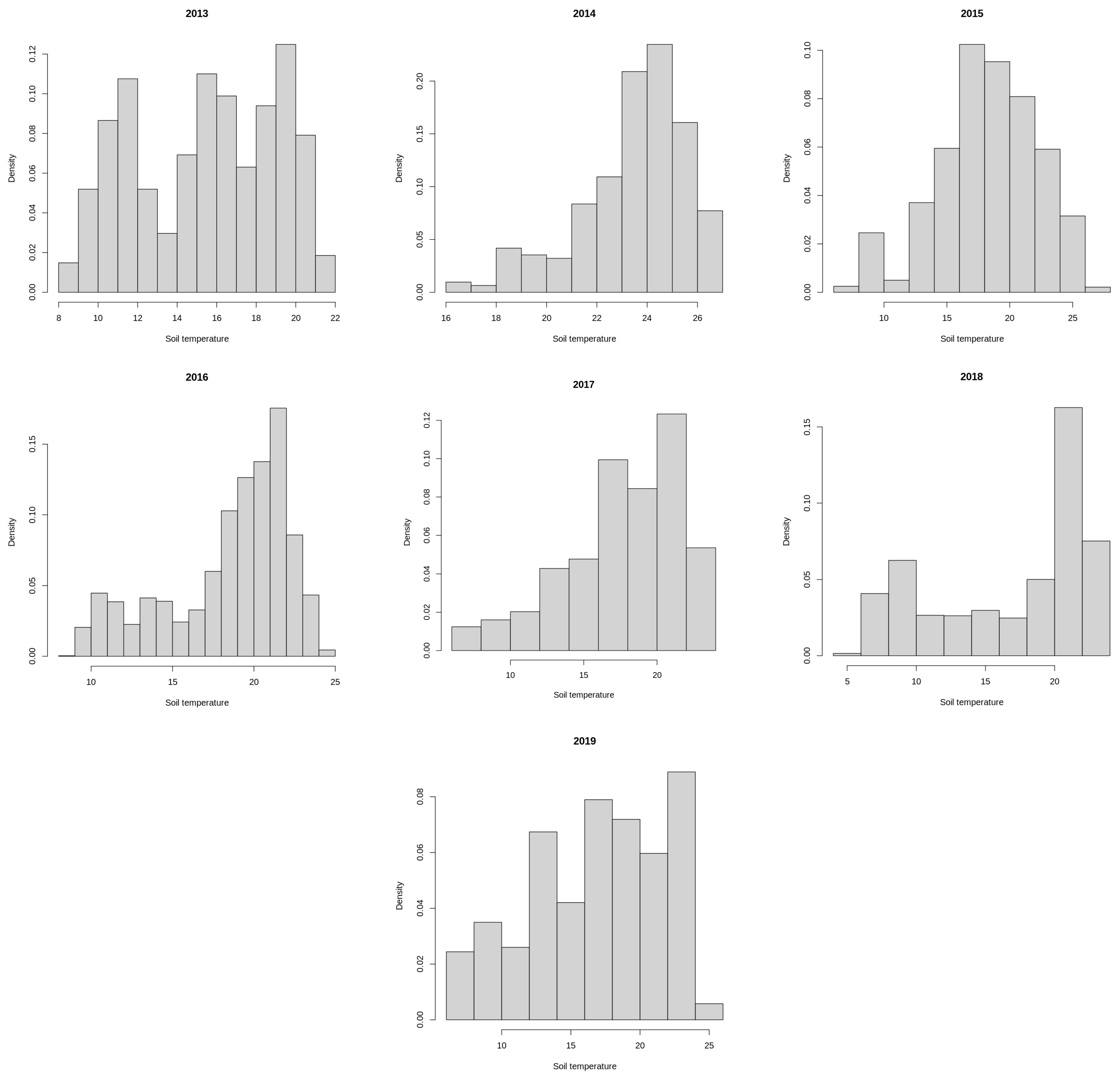
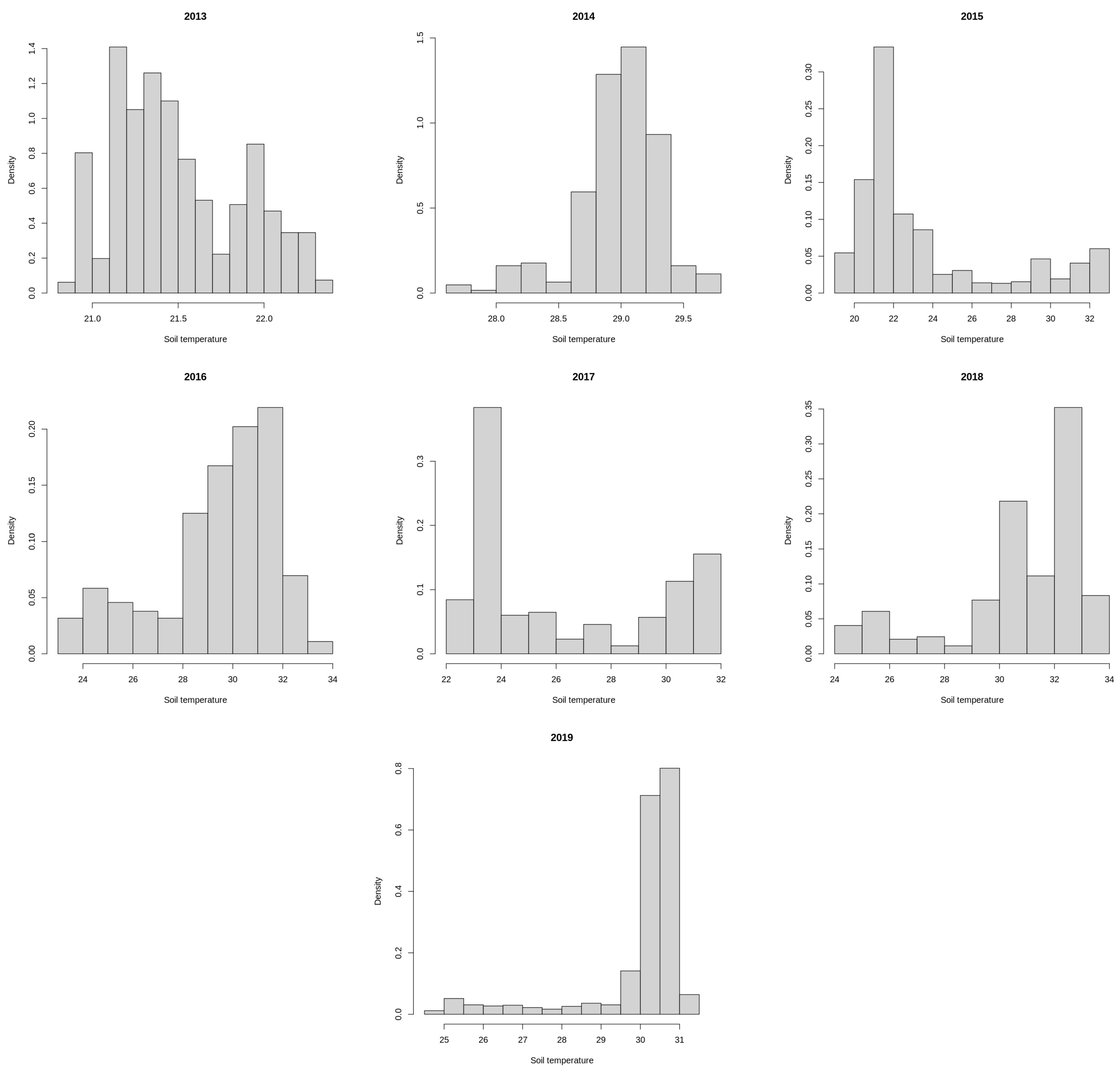
According to the Shapiro–Wilk normality test [31], soil temperature and moisture content observations were not normally distributed (p-values < 0.001). The yearly histograms (Appendix B and Appendix C) also illustrated a significant asymmetry of probability distributions. Preliminary analysis of relationships between climate conditions and two studied soil properties in the monoliths 1 and 2 showed a moderate correlation between air temperature, atmospheric pressure, and the soil temperature at 30 cm (Table 1). The soil moisture content showed no correlation with all climatic indicators.
Due to the problem of stationarity and heteroscedasticity, which was raised by Y. Gao, C. Merz, G. Lischeid, and M. Schneider [18], we tested the hypothesis of a stationary time series of soil properties based on the Augmented Dickey–Fuller Test (ADF) [32]. The test confirmed that both time series for each year were stationary (p-values for the null hypothesis “X is a non-stationary time series” were found less than 0.1). Therefore, considering the revealed statistical properties, we expected the extended ARIMA (p,0,q) models with exogenous climate variables to be suitable for the studied time series.
The following simulated the artificial data gaps—parts of the given time series were randomly dropped with a variation of a gap length from 1 to 50 h. We repeated data gap simulation for each dataset separately (Monolith 1 and Monolith 2) and obtained two samples of gap cases that had different duration varying from short (1–12 h) and middle (13–24 h) to long (25–50 h). In total, we tested 188 gaps, 93 gaps were generated in the time series of soil temperature and 95—in the time series of soil moisture. Simulating data gaps, we supposed that the interval between adjacent data gaps must be more than four days because previous observations have to be used to train the gap-filling routine. Thus, we obtained two random samples of gaps in the time series of soil temperature and moisture for monoliths 1 and 2.

2.3. Methods

The basic idea behind this analysis is to estimate missing values according to a method in each data gap using a dataset within a window covered K complete observations around a data gap. We also supposed that using climatic information can significantly improve gap-filling results. In the first stage, we trained models and estimated missing values for each data gap separately. In the second stage, the idea was to compare the estimated missing values with observed values using the original data and output the goodness of fit indicators.
In this regard, we introduced some notation. Let y(t) be an estimated value within a data gap and t–an index of the calculation period, ordered from 1 to T (the indexes of the first and the last missing values in a data gap). According to this notation, if the observed values yobs(t) are known, the bias error of treated missing values for each t in a data gap can be calculated as
ε(t) = y(t) − yobs(t), t = 1,…,T
We tested the following different methods: (Method 0) simple linear interpolation, (Method 1) multiple linear regression of climate variables, and (Method 2) different variants of extended ARIMA(p,0,q) models with exogenous climate variables.
Method 0. The method of linear interpolation (“zero model”–M0) means simple filling of each data gap with constant growth per hour:
y(t) = y(t − 1) + a, t = 1, 2,…, T
where a–a parameter computed as a = (y(T + 1) − y(0))/(T + 1), y(0) and y(T + 1)—observed values at the beginning and the end a gap, respectively.
Replacing missing values according to Method 0 was considered as a simple and more convenient procedure, which, as expected, gave the worse quality of missing data recovering. However, the accuracy of this method was used to evaluate how other methods performed gap-filling better in the studied time series.
Regression-based imputation methods suppose the replacement of missing values by predicted values from regression estimation. The advantage of these methods is the exploitation of all observations, particularly meteorological data and, in the case of ARIMA models, previous observations to estimate values that are expected under given conditions.
Method 1. The generalized linear model (GLM) recovers missing values based on observed climate variables C(t) in a given period (t = 1, 2, …, T) with a time-of-day component i(t):
y(t) = β·i(t) + a·C(t) + a0
where C(t) = (C1(t),C2(t),…,C6(t))—a vector of independent climate variables including air temperature (°C), air humidity (%), atmospheric pressure (hPa), solar radiation (W/m²), wind speed (m/s), and rainfall (mm); i(t)—a dummy variable associated with the time-of-day; a0, a1,…,a6, β—parameters reflected the effect of independent variables on the outcome variable, computed according to maximum likelihood estimation (MLE).
Due to the revealed stationarity of the time series of soil temperature and moisture, the ARMA model notation as a case of ARIMA (p,0,q) is more suitable to generate values to fill data gaps [18,30,33].
Method 2. The linear autoregressive moving average ARMA(p,q) model with exogenous variables is commonly specified as:
ρ(Lp) (y(t) − a C(t))=φ(Lq) ε(t)
where ρ(Lp) = 1 − ρ1 L − ρ2 L2 − … − ρpLp—the autoregression component AR(p) with an order parameter p, φ(Lq) = 1 + φ1 L+ φ2 L2 + … + φqLq—the moving average component MA(q) with an order parameter q, Lpand Lqare the lag operators with orders of p and q, respectively, in shorthand notation, where Lj = y(tj) indicates the value of y observed at j hours before y(t), a C(t)—linear regression component of independent climate variables notated according to the equation (3).
We tested three variants of the ARMA model: AR(p), MA(q), ARMA(p,q) with adaptive parameters p and q. The orders p and q are given in units of time in a time series. The parameters p and q were optimally selected according to the minimum value of an information criterion Akaike (AIC) from a set of possible orders (p = 0,…,pmax; q = 0,…,qmax).
For each data gap in the studied time series, all models were trained separately. To estimate missing values according to the linear interpolation method (2), we used the start point and the endpoint of a data gap. To learn regression models (3)–(4), training datasets were extracted from the original time series, which had artificial gaps. Each training dataset represents parts of the time series within a window covered K observations before the beginning of a data gap and K observations after and consisted of all climatic variables and observed values of a dependent variable. To identify coefficients of GLM (3), we used the window of 2K observations, as shown in Figure 1. Taking into consideration the specifics of ARMA models, we trained them using K-hours from previous data. Estimation of missing values in a data gap was based on the identified models (3)–(4) using given climatic data for the window size K. We varied K from 2 to 4 days (48 to 96 h) for the models (3) and (4) and found the optimal window size according to the minimum root mean squared error. Figure 1 shows the main principles of trained dataset selection for all used methods.
To compare the performances of modeling procedures for each data gap, we also extracted control datasets from the original data. We used control datasets to estimate the goodness of fit statistics (5)–(7) for each gap in the time series separately.
The mean bias error (MBE):
MBE = t = 1 T ε ( t ) T
The mean absolute error (MAE):
MAE = t = 1 T | ε ( t ) | T
The root mean squared error (RMSE):
RMSE = t = 1 T ε ( t ) 2 T
The mean absolute percentage error (MAPE):
MAPE = t = 1 T | ε ( t ) | | y o b s ( t ) | 1 T
All calculations were performed using R with packages “forecast”, “aTSa” and “lubridate”. To estimate coefficients of ARIMA (p,0,q) models and select optimal order parameters p and q, we used the auto.arima() function from a package “forecast” with stepwise selection option (stepwise = TRUE), which allowed us to exclude insignificant independent variables.

3. Results and Discussion

Following the data gap-filling procedure, we estimated coefficients in regression models (3)–(4) and obtained predicted values for each missing value. In particular, the computation results revealed that the input of the time-of-day variables and climate information significantly improved regression models. The statistical significance of climate variables varied depending on a gap length and climate conditions. The hourly sum of precipitation and the wind speed were insignificant factors to predict soil temperature at topsoil. Thus, these variables were dropped out from the specification of this model. Despite no correlation between soil moisture and climate data, some of the climate variables were statistically significant in soil moisture regression models. The exception was the precipitation, which was excluded from all regression models. The list of significant variables was different for gaps and was not of interest to our study. As preliminary calculations showed, the maximum values of optimal order parameters p and q for AR (p), MA (q), and ARMA (p,q) models were 5 and 3, respectively. Therefore, to minimize computation time, optimization of order parameters was conducted by varying p from 0 to 5 and q from 0 to 3. In total, for 188 data gaps, we identified 188 GLM models and 564 ARMA models. For each model, we found the optimal window size (K); and for ARMA models, optimal values of p and/or q were computed, as well.

3.1. Mean Error Analysis

To compare gap-filling techniques, we calculated the means of the bias error indicators (MBE, MAE, RMSE, and MAPE) for all methods (Table 2).
The results showed that ARMA (p,q) model had significant advantages in gap-filling in the time series of the soil temperature at 30 cm. The mean bias error produced by the extended ARMA model ranged from −0.70 to 1.02 °C and had a mean value of −0.02 °C with a standard deviation of 0.19. Compared to multiple linear regression and simple linear interpolation, the accuracy of missing values estimations based on the ARMA model was significantly better. For example, MBE for linear regression varied from −2.1 to 1.94 °C with a mean value of 0.04 °C and a standard deviation of 0.47 °C. The minimum of the mean absolute error (0.19 °C) was also achieved using the ARMA model, while MAEs generated by linear interpolation and linear regression were about two times higher. According to MAPE, the lost information in data recovery decreased from 2.4% in the linear interpolation to 1.3% on average for the ARMA model. However, the maximum values of MAPE reached 10.7%, 14.4%, 15.0%, 16.6%, and 10.1% for the linear interpolation, multiple linear regression, AR (p), MA (q), and ARMA (p,q) models, respectively.
Regarding soil moisture, the bias error analysis showed that the ARMA model had moderate advantages over other missing value imputation methods in general. The MAPE (0.33%) and RMSE (0.10 Vol. %) were less than in other cases. The MBE for the ARMA model was 0.01 Vol. % with a standard deviation of 0.1 Vol. % and ranged from −0.27 to 0.80 Vol. %. The ARMA model produced more accurate results than simple linear interpolation for which MBE varied from −0.55 to 0.51 Vol. % with −0.003 Vol. % of mean value and 0.11 of standard deviation. We should note that MA (q) model was the worst variant of gap-filling techniques producing the highest bias errors. Moreover, the advantages of the ARMA model became clear when we analyzed the maximum values of MAPE. ARMA model produced maximum 2.1% of MAPE, AR (p)—8.2%, MA (q)—16.0%, GLM—3.4%, and the linear interpolation—2.3%.
The mode values for the optimal orders of ARMA (p,q) were 2 and 0 for p and q in both soil temperature and moisture content models. The average optimal window size to get accurate prediction was 71 h of previous observations.
These findings confirmed the high suitability of the ARMA model to the nature of soil temperature and moisture content dynamics.

3.2. Error Analysis in Gap Size Class

To compare the performance of methods in relation to gap size classes, we estimated MAEs and their standard deviations for each gap length (Table 3). The results showed the different power of the models in missing value estimation.
The best technique of gap filling in soil temperature time series, as mentioned above, was also the ARMA model with the lowest MAEs and standard deviations for all gap classes. MAE for short gaps (<13 h) was 0.06 °C with a standard deviation of 0.06 °C. The missing values in middle-length gaps can be estimated with an expected error of 0.16 °C with a standard deviation of 0.13 °C. Long-length gaps can be filled with an expected accuracy of 0.26 °C and its standard deviation 0.19 °C. These values were significantly smaller than the standard deviations of hourly soil temperature in given months. MAEs decreased by half in extended ARMA models due to adding climate information. We should also note that the adaption of order parameters in the ARMA model played a crucial role in improving gap-filling results.
The filling of short-length gaps in soil moisture time series produced better results via simple AR (p) and ARMA (p,q) models, according to MAE–0.04 and 0.03 Vol.%, respectively. These models had moderate advantages in filling data gaps due to lower MAEs and standard deviations. Estimating missing values in middle-length gaps was done with an expected accuracy of 0.07 Vol. % and the standard deviation of 0.06–0.07 Vol. %. The input of climate information did not significantly decrease the error for long-length gaps (25–50 h), which reached 0.11 Vol. % on average.
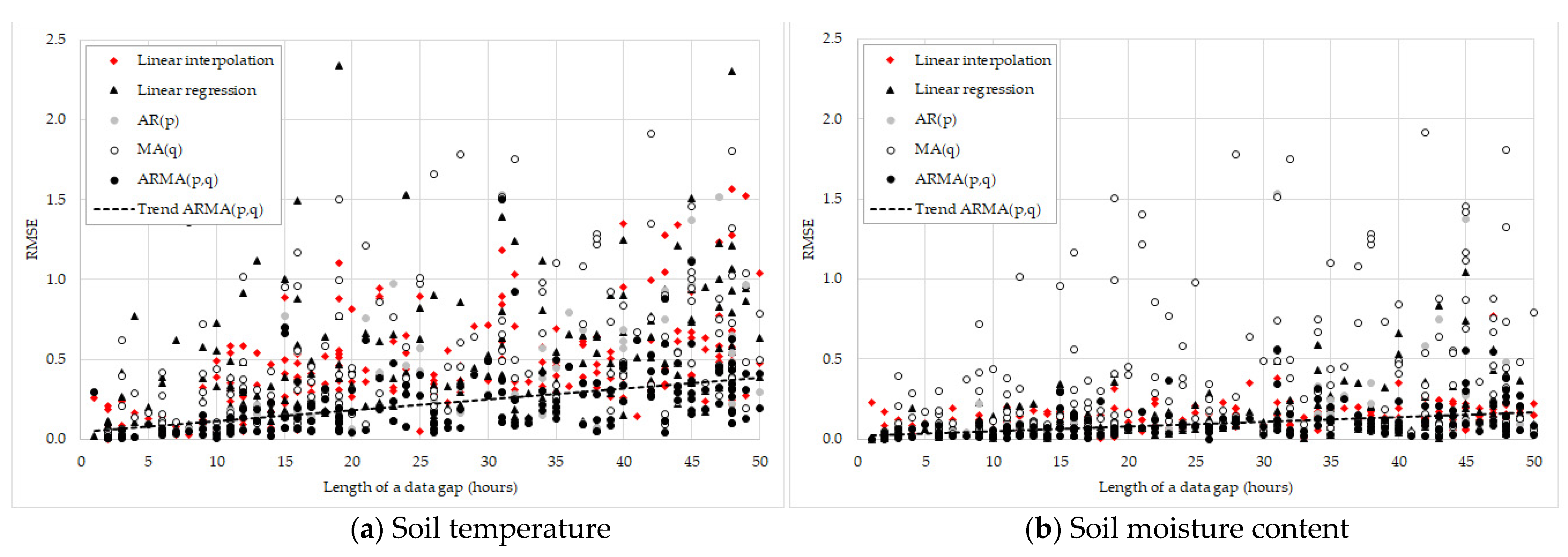
Figure 2 presents the general dependence of RMSEs on data gap lengths. Linear interpolation, GLM, MA (q), and AR (p) models produced higher RMSE with high variance compared to ARMA models. Importantly, ARMA models were generally better than other methods for all gap durations for soil temperature time series. Regarding soil moisture, we also observed an increasing RMSE, depending on the gap length and the advantage of ARMA models.
Comparisons of missing value estimations for two studied land use systems showed insignificant differences in the mean bias error between arable land (Monolith 1) and natural steppe vegetation (Monolith 2). p-values of t-test comparing two means MBE for the null hypothesis were more than 0.1 for all methods of gap-filling. Nonetheless, the analysis of MAPEs showed moderate differences in accuracy of estimations (Table 4).

3.3. Examples of Gap Filling and Selection of the Best Model

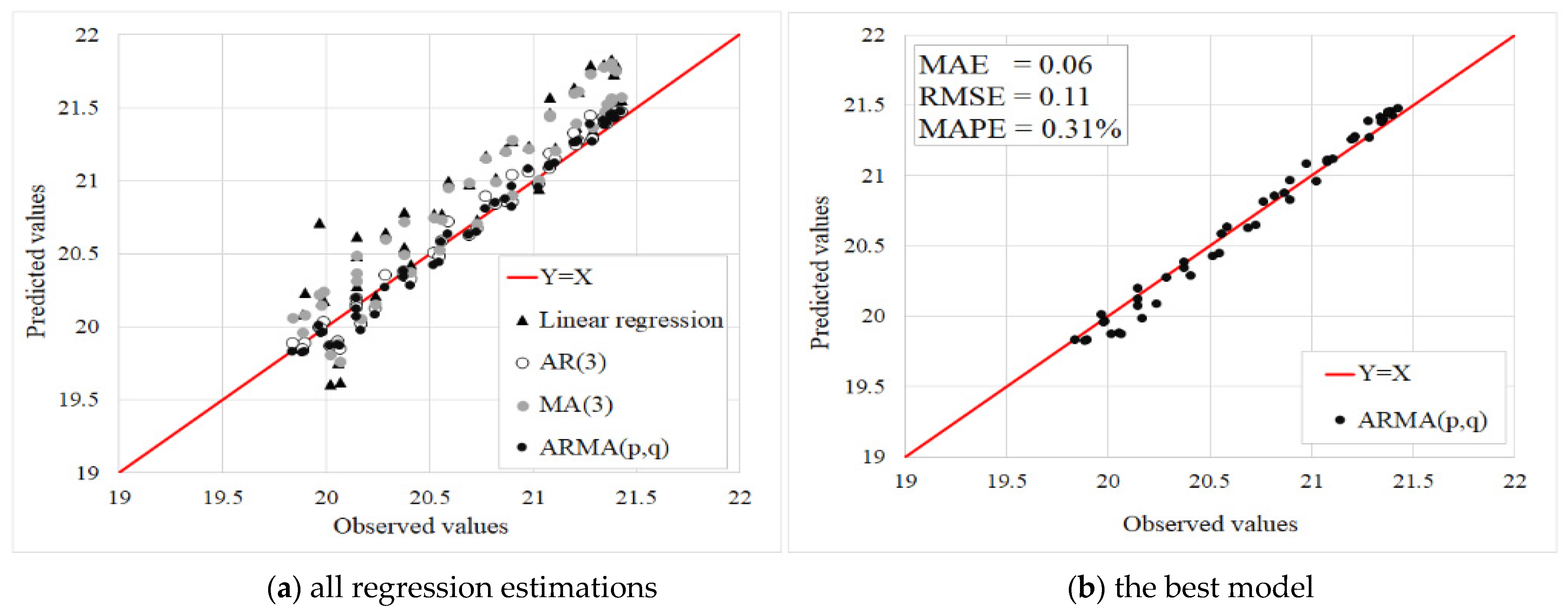
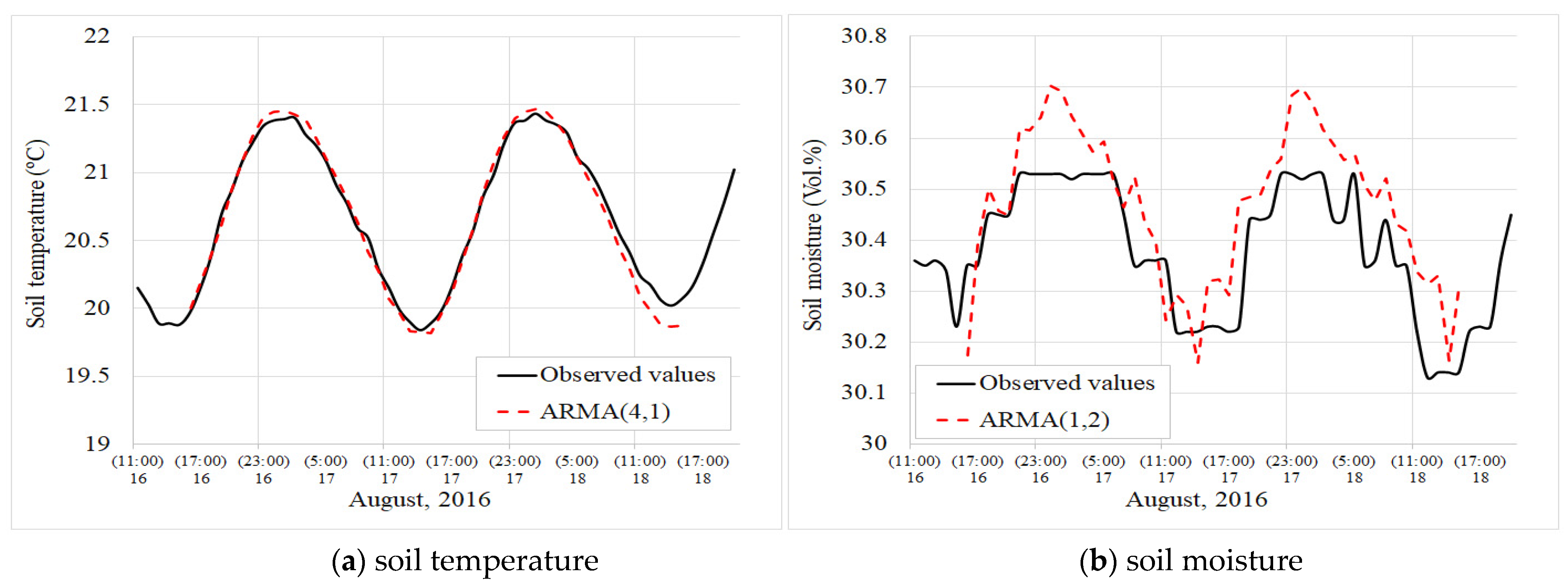
To illustrate the effectiveness of the gap-filling routines, two examples of missing value estimation are presented. Figure 3 presents the examples of missing value estimations for a long-length gap (48 h) in time series of the soil temperature. According to a common approach, the best model has to give estimations closest to actual values. In the present case, the best filling model was ARMA (4,1), which produced MAE equal to 0.06 °C and MAPE–0.31%.
As shown in Figure 4, the regression estimation of missing values in soil moisture time series had a high deviation, but the best models were ARMA (1,2) produced MAE–0.095 Vol. % and MAPE–0.31%.
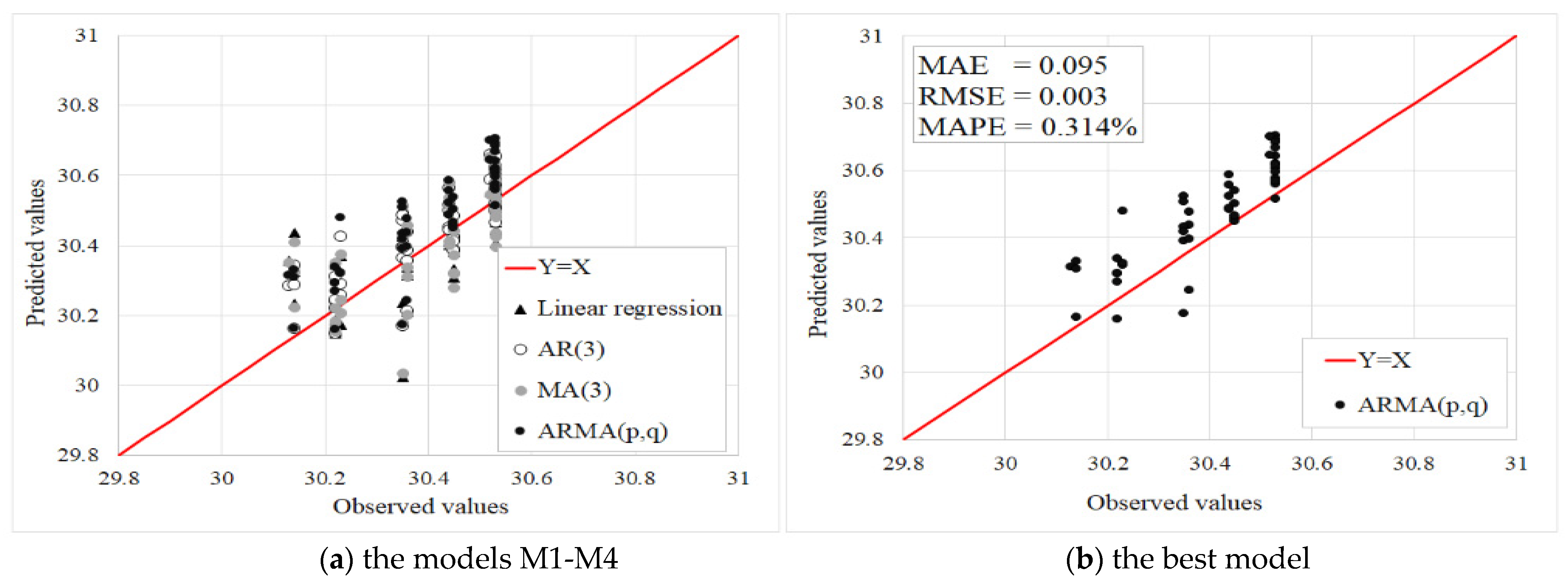
Figure 5 graphically represents the fitting of the observed and estimated values according to the best model for both cases. Generally, the ARMA model showed a good agreement with observed soil temperature values while this model demonstrated the minor effect of overestimation in long-term gap filling of soil moisture time series.
The results showed that MA (q) models were the least effective in gap-filling. The multiple linear regression models gave us low accuracy of estimations, even with the time-of-day variables, and can hardly be considered as a good tool of data gap filling in soil hydrological measurements. As was noted by Gao Y., Merz C., Lischeid G., and Schneider M. [18], regression methods tend to overestimate correlations and decrease variance. Moreover, according to a similar study [34], gap-filling in hourly time series of soil moisture showed the highest RMSE compared to other techniques. Simple techniques, such as replacement by monthly average, showed significantly better results. Linear interpolation cannot principally describe dynamics of soil hydrological settings during the day, which is important for using such estimations, especially if we face long-length gaps. Notably, the effectiveness of gap-filling methods with adaptive parameters such as ARMA (p,q) is limited if serial gaps become frequent and happen more often than 72 h [35].

4. Conclusions

Missing data comprise a common problem in meteorological and hydrological studies, which causes substantial difficulties for most statistical models, decreases the effectiveness of introducing online digital tools in agriculture. In this study, we compared various gap-filling methods in the time series of topsoil properties measured by the lysimeter station for two cases–arable land and natural steppe vegetation during vegetation periods of 2013–2019. Here, we applied different methods from conventional multiple linear regression practices and linear interpolation to the more sophisticated method—the extended ARMA model with exogenous climate variables. Despite the relatively low MAEs of gap-filling and the simplicity of the method, linear interpolation cannot describe non-linear hourly dynamics of soil temperature and moisture, especially if a gap length is longer than 6 h. Multiple linear regression and MA (q) models showed lower accuracy compared to the extended ARMA model. We confirmed that the ARMA model with exogenous climate variables has some advantages for missing values estimation in both soil time series under different climatic conditions. First of all, the considered approach has benefits, due to adaptive parameters of autoregressive and moving average components (p,q), and the adaptive window (K). Moreover, the input of climate information into the ARMA model demonstrated a significant improvement. Therefore, the ARMA (p,q) model can be used as a good tool for the prediction of soil properties and their dynamics, based on known climatic data and a part of the previous observations. This is important in case of short-term equipment failure. However, the ARMA(p,q) model has some disadvantages: first, demand for sufficient dataset to train a model; second, the dependence of results on a criterion of selecting optimal parameters p and q. Here, we used AIC to select the optimal order parameters. Further studies will be challenged with at least three problems: the first criterion justification to select the best ARMA(p,q) model; the second analysis of gap-filling methods performance using a wider set of climatic events from droughts to more humid conditions, and a winter season; the third comparisons of the gap-filling effectiveness using various ARIMA, ARCH and GARCH models, as well as neural networks.

Author Contributions

These authors contributed equally to this work. All authors have read and agreed to the published version of the manuscript.

Funding

The paper was based on research studies, which have been funded by the German Federal Ministry of Education and Research (BMBF) in the framework of the former project KULUNDA for 2013-2016 (FKZ 01LL0905D) and the running project ReKKS (FKZ 01LZ1704C). The study was also supported by the state assignment of the Altai State University “The Turkic World of the Large Altai: Unity and Diversity in History and Modernity” (project number–748715F.99.1.BB97AA00002).

Acknowledgments

The authors would like to thank their colleagues from Martin Luther University Halle-Wittenberg, Institute of GeoSciences and Geography, namely, Gerd Schmidt, Moritz Koza, Michael Zierdt, and Dorothee Kley. The authors would also like to express gratitude to the colleagues from Helmholtz Centre for Environmental Research (UFZ), Ralph Meissner, and Lisa Haselow for scientific support of this study, discussions, and an opportunity to continue our study after the Kulunda project was finished. We acknowledge the managers of the farm “Partner” in the village of Poluyamki, the Kozhanov family, and the agronomist Nikolay Rudev, who provided the installation of the monitoring network and its functioning. We also want to thank Associate Professor Vsevolod Shcherbinin from the Altai State University for the monitoring network’s technical services during 2013–2016. We also thank the three anonymous reviewers, whose recommendations and remarks helped us improve the manuscript.

Conflicts of Interest

The authors declare no conflict of interest.

Appendix A

Table A1. The climatic conditions and descriptive statistics of soil temperature and soil moisture at the 30 cm depth during the vegetation period (May–September) for 2013–2019, Poluyamki, Altai Krai, Russia.
Used Statistic2013 12014 22015 32016 32017 42018 42019 4
The weather station
Air temperature (°C)Mean
(St. dev.)
13.5
(7.0)
24.5
(5.5)
18.0
(7.0)
17.8
(6.8)
18.6
(7.0)
17.1
(7.7)
16.7
(7.4)
Air humidity (%)Mean
(St. dev.)
60.8
(21.8)
40.6
(16.8)
54.4
(19.8)
56.1
(21.2)
50.7
(19.8)
56.6
(20.1)
49.5
(19.7)
Solar radiation (W/m2)Mean
(St. dev.)
159.4
(226.6)
286.1
(325.2)
229.4
(294.1)
234.1
(297.8)
264.0
(321.1)
248.2
(313.6)
267.3
(321.3)
Wind speed (m/s)Mean
(St. dev.)
2.5
(1.6)
2.8
(1.8)
2.8
(1.8)
2.4
(1.7)
2.9
(1.8)
2.8
(1.8)
1.9
(1.9)
Atmospheric pressure (hPa)Mean
(St. dev.)
996.5
(7.9)
991.9
(3.4)
993.6
(7.1)
994.3
(7.3)
993.0
(7.1)
991.2
(6.4)
994.5
(7.5)
Precipitation (mm)Sum37.84.4243.2325.1151.1219.487.1
The lysimeter station, measurements at 30 cm
Soil temperature (°C)
Arable land (Monolith 1)Mean
(St. dev.)
15.4
(3.5)
23.5
(2.1)
18.3
(3.9)
18.5
(3.8)
17.7
(3.9)
16.9
(5.5)
16.9
(4.8)
Grass land (Monolith 2)Mean
(St. dev.)
14.6
(3.1)
20.6
(1.9)
16.6
(3.4)
16.5
(3.5)
15.9
(3.9)
14.5
(5.0)
14.3
(4.0)
Soil moisture (Vol.-%)
Arable land (Monolith 1)Mean
(St. dev.)
21.5
(0.4)
28.9
(0.3)
23.6
(3.8)
29.4
(2.3)
26.2
(3.4)
30.7
(2.3)
29.9
(1.4)
Grass land (Monolith 2)Mean
(St. dev.)
18.7
(0.3)
18.8
(0.18)
18.9
(2.3)
22.8
(4.9)
22.9
(4.9)
28.1
(5.7)
23.7
(4.6)
Available data: 1—from August to September in 2013; 2—June of 2014; 3—from May to September in 2015 and 2016; 4—from May to August in 2017, 2018 and 2019. Calculated by the authors based on hourly data from WS and LYS, Poluyamki, Altai Krai, Russia.

Appendix B

Figure A1. Distribution of soil temperature measurements at 30 cm, the arable land monolith, the lysimeter station for 2013–2019, Poluyamki, Altai Krai, Russia. Available data from August to September in 2013; June of 2014; from May to September in 2015 and 2016; from May to August in 2017, 2018 and 2019. Calculated by the authors based on hourly data from LYS.
Land 10 00579 g0a1

Appendix C

Figure A2. Distribution of soil moisture measurements at 30 cm, the arable land monolith, the lysimeter station for 2013–2019, Poluyamki, Altai Krai, Russia. Available data from August to September in 2013; June of 2014; from May to September in 2015 and 2016; from May to August in 2017, 2018 and 2019. Calculated by the authors based on hourly data from LYS.
Land 10 00579 g0a2

References

  1. Food and Agriculture Organization of the United Nations (FAO). Drought-Resistant Soils: Optimization of Soil Moisture for Sustainable Plant Production. FAO Land and Water Bulletin 11. Available online: http://www.fao.org/3/a0072e00.htm#Contents (accessed on 2 October 2020).
  2. Beliaev, V.; Grunwald, L.; Meinel, T.; Schmidt, G.; Bondarovich, A.A.; Scherbinin, V.V.; Ponkina, E.V.; Matsyura, A.V.; Stephan, E.; Illiger, P.; et al. Soil water regime and crop yields in relation to various technologies of cultivation in the Kulunda Steppe (Altai Krai). Vis. Dnipropetr. Univer. Biol. Ecol. 2016, 24, 531–539. [Google Scholar] [CrossRef]
  3. Belyaev, V.I.; Meinel, T.; Meissner, R.; Grunwald, L.-C.; Volnov, V.V.; Stephan, E.; Sokolova, L.V. Autumn Tillage, Soil Moisture Content, and Crop Yields. In Kulunda: Climate Smart Agriculture; Frühauf, M., Guggenberger, G., Meinel, T., Theesfeld, I., Lentz, S., Eds.; Springer Nature Switzerland AG: Cham, Switzerland, 2020; pp. 355–366. [Google Scholar] [CrossRef]
  4. Sadras, V.O.; Villalobos, F.J.; Orgaz, F.; Fereres, E. Effects of Water Stress on Crop Production. In Principles of Agronomy for Sustainable Agriculture; Villalobos, F.J., Fereres, E., Eds.; Springer Nature Switzerland AG: Cham, Switzerland, 2016; pp. 189–204. [Google Scholar] [CrossRef]
  5. Cook, F.J.; Orchard, V.A. Relationships between soil respiration and soil moisture. Soil Biol. Biochem. 2008, 40, 1013–1018. [Google Scholar] [CrossRef]
  6. Food and Agriculture Organization of the United Nations (FAO). Crop Evapotranspiration—Guidelines for Computing Crop Water Requirements—FAO Irrigation and Drainage Paper 56; Allen, R.G., Pereira, L.S., Raes, D., Smith, M., Eds.; Food and Agriculture Organization of the United Nations (FAO): Rome, Italy, 1998. [Google Scholar]
  7. Bondarovich, A.A.; Scherbinin, V.V.; Ponkina, E.V.; Matsyur, A.; Puzanov, A.; Stephan, E.; Balykin, D.; Rupp, H.; Meissner, R. Soil Moisture and Evapotranspiration. In Kulunda: Climate Smart Agriculture; Frühauf, M., Guggenberger, G., Meinel, T., Theesfeld, I., Lentz, S., Eds.; Springer Nature Switzerland AG: Cham, Switzerland, 2020; pp. 167–181. [Google Scholar] [CrossRef]
  8. Meissner, R.; Rupp, H.; Bondarovich, A.A.; Rinklebe, J. Soil water management in the Siberian Kulunda—Dry steppe. Mechaniz. Agric. Conser. Res. 2017, 63, 197–201. Available online: https://stumejournals.com/journals/am/2017/5/197 (accessed on 2 October 2020).
  9. Ihuoma, S.O.; Madramootoo, C.A. Recent advances in crop water stress detection. Comput. Electron. Agric. 2017, 141, 267–275. [Google Scholar] [CrossRef]
  10. Lisar, S.Y.S.; Motafakkerazad, R.; Mosharraf, M.H.; Rahman, I.M.M. Water Stress in Plants: Causes, Effects and Responses. In Water Stress; Mofizur, R.I., Ed.; Intech Open Limited: London, UK, 2012; pp. 1–16. [Google Scholar] [CrossRef] [Green Version]
  11. Bavorova, M.; Imamverdiyev, N.; Ponkina, E. Farm-level economics of innovative tillage technologies: The case of no-till in the Altai Krai in Russian Siberia. Envir. Sci. Pollut. Res. 2018, 25, 1016–1032. [Google Scholar] [CrossRef] [PubMed]
  12. Balykin, D.; Puzanov, A.; Stephan, E.; Meissner, R. Using the Innovative Lysimeter Technology in The German–Russian Research Project “KULUNDA”. In Novel Methods for Monitoring and Managing Land and Water Resources in Siberia; Mueller, L., Sheudshen, A.K., Eulenstein, F., Eds.; Springer Nature Switzerland AG: Cham, Switzerland, 2016; pp. 387–399. [Google Scholar] [CrossRef]
  13. Frühauf, M.; Guggenberger, G.; Meinel, T.; Theesfeld, I.; Lentz, S. (Eds.) Kulunda: Climate Smart Agriculture; Springer Nature Switzerland AG: Cham, Switzerland, 2020; Available online: https://www.springer.com/gp/book/9783030159269#otherversion=9783030159276 (accessed on 2 October 2020).
  14. Nolz, R.; Kammerer, G.; Cepuder, P. Interpretation of lysimeter weighing data affected by wind. Soil Sci. Plant Nutr. 2013, 176, 200–208. [Google Scholar] [CrossRef]
  15. Peters, A.; Nehls, T.; Schonsky, H.; Wessolek, G. Separating precipitation and evapotranspiration from noise: A new filter routine for high-resolution lysimeter data. Hydrol. Earth Syst. Sci. 2014, 18, 1189–1198. [Google Scholar] [CrossRef] [Green Version]
  16. Schmidt, A.; Wrzesinsky, T.; Klemm, O. Gap Filling and Quality Assessment of CO2 and Water Vapour Fluxes above an Urban Area with Radial Basis Function Neural Networks. Bound. Layer Meteorol. 2008, 126, 389–413. [Google Scholar] [CrossRef]
  17. Fleischer, E.; Khashimov, I.; Hölzel, N.; Klemm, O. Carbon exchange fluxes over peatlands in Western Siberia: Possible feedback between land-use change and climate change. Sci. Total Environ. 2016, 545, 424–433. [Google Scholar] [CrossRef] [PubMed]
  18. Gao, Y.; Merz, C.; Lischeid, G.; Schneider, M. A review on missing hydrological data processing. Environ. Earth Sci. 2018, 77, 47. [Google Scholar] [CrossRef]
  19. Velikanova, L.I.; Lychenko, N.M. Recovering of data gaps in time series of temperature based on artificial neural networks. Probl. Auto. Contr. 2018, 35, 51–58. [Google Scholar]
  20. Gold, L.W. Analysis of annual variations in ground temperature at an Ottawa site. Can. J. Earth Sci. 1964, 1, 146–157. [Google Scholar] [CrossRef]
  21. Lamba, B.S.; Khambete, N.N. Analysis of subsoil temperature at various depths by Fourier technique. Mausam 1991, 42, 269. [Google Scholar]
  22. Bromba, M.U.A.; Ziegler, H. Application hints for Savitzky-Golay digital smoothing filters. Anal. Chem. 1981, 53, 1583–1586. [Google Scholar] [CrossRef]
  23. Falge, E.; Baldocchi, D.; Olson, R.; Anthoni, P.; Aubinet, M.; Bernhofer, C.; Burba, G.; Ceulemans, R.; Clement, R.; Dolman, H.; et al. Gap filling strategies for defensible annual sums of net ecosystem exchange. Agr. For. Meteorol. 2001, 1, 43–69. [Google Scholar] [CrossRef] [Green Version]
  24. Adeniyi, M.O.; Nymphas, E.F. Estimation of bare soil surface temperature from air temperature and soil depth temperature in a tropical station. Int. J. Nat. Appl. Sci. 2011, 4, 429–437. [Google Scholar]
  25. Asgharinia, S.; Petroselli, A. A comparison of statistical methods for evaluating missing data of monitoring wells in the Kazeroun Plain, Fars Province, Iran. Groundw. Sustain. Dev. 2020, 10, 100294. [Google Scholar] [CrossRef]
  26. Astel, A.; Mazerski, J.; Polkowska, Ż.; Namieśnik, J. Application of PCA and time series analysis in studies of precipitation in Tricity (Poland). Adv. Environ. Res. 2004, 8, 337–349. [Google Scholar] [CrossRef]
  27. Machiwal, D.; Jha, M.K. Comparative evaluation of statistical tests for time series analysis: Application to hydrological time series. Hydrol. Sci. J. 2008, 53, 353–366. [Google Scholar] [CrossRef]
  28. Haselow, L.; Meissner, R.; Rupp, H.; Miegel, K. Evaluation of precipitation measurements methods under field conditions during a summer season: A comparison of the standard rain gauge with a weighable lysimeter and a piezoelectric precipitation sensor. J. Hydrol. 2019, 575, 537–543. [Google Scholar] [CrossRef]
  29. Abramenkova, I.V.; Kruglov, V.V. Methods of gap recovering in datasets. Soft Syst. 2005, 2, 18–22. [Google Scholar]
  30. Brockwell, P.J.; Davis, R.A. Time Series: Theory and Methods, 2nd ed.; Springer Nature Switzerland AG: Cham, Switzerland, 2006. [Google Scholar]
  31. Shapiro-Wilk Normality Test. 2020. Available online: https://www.rdocumentation.org/packages/stats/versions/3.6.2/topics/shapiro.test (accessed on 2 October 2020).
  32. Augmented Dickey-Fuller Test. 2020. Available online: https://www.rdocumentation.org/packages/aTSA/versions/3.1.2/topics/adf.test (accessed on 2 October 2020).
  33. Box, G.E.P.; Jenkins, G.M.; Reinsel, G.C. Time Series Analysis: Forecasting and Control, 4th ed.; John Wiley: New York, NY, USA, 2008. [Google Scholar]
  34. Gift, D.; Coulibaly, P. Evaluation of statistical methods for infilling missing values in high-resolution soil moisture data. J. Hydrol. 2011, 400, 95–102. [Google Scholar] [CrossRef]
  35. Kornelsen, K.; Coulibaly, P. Comparison of Interpolation, Statistical, and Data-Driven Methods for Imputation of Missing Values in a Distributed Soil Moisture Dataset. J. Hydrol. Eng. 2014, 19, 26–43. [Google Scholar] [CrossRef]
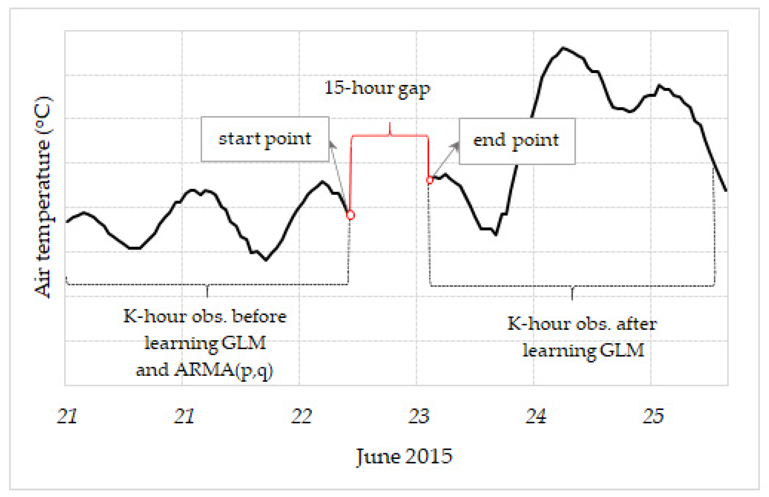
Figure 1. The main principles of trained data selection depending on the used methods. Source: authors.
Land 10 00579 g001
Figure 2. The dependence of RMSE on data gap length (N = 188). Calculated by the authors based on hourly time series for 2013–2019, the data of monitoring network in Poluyamki, Altai Krai, Russia.
Land 10 00579 g002
Figure 3. The case of missing value estimation in the time series of soil temperature (°C), 48 h data gap length, 16–18 August 2016. Calculated by the authors based on hourly time series, the data of monitoring network in Poluyamki, Altai Krai, Russia.
Land 10 00579 g003
Figure 4. The case of missing value estimation in the time series of soil moisture (Vol. %), 48 h data gap length, 16–18 August 2016. Calculated by the authors based on the hourly time series, the data of monitoring network in Poluyamki, Altai Krai, Russia.
Land 10 00579 g004
Figure 5. An example of 48 h length gaps filling via the extended ARMA model with exogenous climate variables. Calculated by the authors based on hourly time series, the data of monitoring network in Poluyamki, Altai Krai, Russia.
Land 10 00579 g005
Table 1. The Spearman’s rank correlation between climate parameters (WS) and soil indicators measured at 30 cm.
Air Temperature (°C)Air Humidity (%)Atmospheric Pressure (hPa)Solar Radiation (W/m²)Wind Power (m/sec)Rainfall (mm)
Soil temperature (°C)
Arable land (Monolith 1)0.51 *0.13 *−0.51 *−0.04−0.19 *−0.02
Natural steppe vegetation (Monolith 2)0.52 *0.16 *−0.50 *−0.01−0.16 *−0.01
Soil moisture content (Vol.−%)
Arable land (Monolith 1)0.01−0.04 *−0.05 *0.04 *0.002−0.007
Natural steppe vegetation (Monolith 2)−0.11 *−0.06 *0.020.07 *0.08 *0.02
*—a p-value < 0.001, probability of the null hypothesis, according to the z-test. Calculated by the authors based on hourly time series for 2013–2019, the data of monitoring network in Poluyamki, Altai Krai, Russia.
Table 2. Mean errors of missing values reconstruction in the time series of soil temperature and moisture via different methods; measurements at the 30 cm depth; monoliths 1 and 2.
Linear InterpolationLinear RegressionAR (p)MA (q)ARMA (p,q)
Soil temperature (°C)
MBE0.030.040.03−0.06−0.02
MAE0.390.430.270.450.19
RMSE0.450.490.310.520.23
MAPE2.39%2.77%1.76%2.97%1.31%
Average optimal window size (hours)67676871
Soil moisture content (Vol.%)
MBE0.01−0.0030.04−0.010.01
MAE0.100.120.110.350.08
RMSE0.130.150.130.410.10
MAPE0.42%0.47%0.57%2.04%0.33%
Average optimal window size (hours)56725971
The bold font indicates a minimum absolute value in each line. Calculated by the authors based on hourly time series for 2013–2019, the data of monitoring network in Poluyamki, Altai Krai, Russia. N = 188.
Table 3. The mean absolute error (MAE) of the soil properties estimations via different methods depending on the length of data gaps; measurements at the 30 cm depth of the arable land (Monolith 1); natural steppe vegetation (Monolith 2); mean (standard deviation).
Gap-Length ClassesLinear InterpolationLinear Regression AR (p)MA (q)ARMA (p,q)
Soil temperature (°C)
Short0.170.250.070.240.06
(0.15)(0.22)(0.07)(0.25)(0.06)
Middle0.390.410.210.380.16
(0.20)(0.39)(0.21)(0.32)(0.13)
Long0.470.500.380.570.26
(0.28)(0.33)(0.30)(0.40)(0.19)
Soil moisture content (Vol. %)
Short0.070.060.040.170.03
(0.05)(0.05)(0.03)(0.19)(0.02)
Middle0.090.090.070.310.07
(0.06)(0.07)(0.06)(0.33)(0.07)
Long0.130.160.160.450.11
(0.08)(0.15)(0.21)(0.42)(0.10)
The bold font indicates a minimum value in each line. Calculated by the authors based on hourly time series for 2013–2019, the data of monitoring network in Poluyamki, Altai Krai, Russia.
Table 4. The mean absolute percentage error (MAPE) of the missing values estimations via different methods depending on the land use, measurements at the 30 cm depth; mean (%).
NLinear InterpolationLinear RegressionAR (p)MA (q)ARMA (p,q)
Soil temperature (°C)
Arable land (Monolith 1)933.163.411.953.291.62
Grassland (Monolith 2)951.652.672.532.671.02
Soil moisture content (Vol. %)
Arable land (Monolith 1)930.470.580.773.250.35
Grassland (Monolith 2)950.370.440.340.900.25
The bold font indicates a minimum value in each line. Calculated by the authors based on hourly time series for period 2013–2019, the data of monitoring network in Poluyamki, Altai Krai, Russia.
Publisher’s Note: MDPI stays neutral with regard to jurisdictional claims in published maps and institutional affiliations.