GHG Balance of Agricultural Intensification & Bioenergy Production in the Orinoquia Region, Colombia

Abstract

Energy crop expansion can increase land demand and generate displacement of food crops, which impacts greenhouse gas (GHG) emissions mainly through land-use change (LUC). Increased agricultural productivity could compensate for this. Our study aims to evaluate the regional combined GHG emissions of increasing agricultural yields for food crop and beef production and using the generated surplus land for biomass production to replace fossil fuels in the Orinoquia region of Colombia until 2030. The results show that surplus land for biomass production is obtained only when strong measures are applied to increase agricultural productivity. In the medium and high scenario, a land surplus of 0.6 and 2.4 Mha, respectively, could be generated. Such intensification results in up to 83% emission reduction in Orinoquia’s agricultural sector, largely coming from increasing productivity of cattle production and improving degraded pastures. Biofuel potential from the surplus land is projected at 36 to 368 PJ per year, with a low risk of causing indirect LUC, and results in GHG emission reductions of more than 100% compared to its fossil fuel equivalent. An integrated perspective of the agricultural land use enables sustainable production of both food and bioenergy.

1. Introduction

Based on the need to reduce fossil fuel consumption and GHG emissions, bioenergy production has increased in the past decades and it is projected to continue to grow [1]. However, expansion of energy crop production could incur increased land demand, and thereby increase greenhouse gas (GHG) emissions due to direct and indirect land-use change ((I)LUC) [2]. To minimize these effects, the sustainability criteria of the Renewable Energy Directive (RED II) require low-ILUC risk-biofuels and minimum GHG emission savings compared to the fossil fuel equivalent [2]. Biofuels are considered to have a low-ILUC-risk, when energy crops are cultivated on surplus land that can be made available due to the implementation of measures to further increase yields of agricultural production compared to a business-as-usual scenario [3]. Producing energy crops at surplus land obtained through agricultural intensification reduces the risk of LUC and (I)LUC related GHG emissions [4,5,6].

Colombia has been promoting the development of a sustainable biomass and bioenergy sector in the last decade [7]. The efficient use of agricultural land has been an important objective of development, as current agricultural land use has low productivity and there is a potential risk the agricultural sector continues to develop in an inefficient way [8,9,10]. The Ministry of Agriculture and Rural Development recently delimited the agricultural frontier, indicating which land could potentially be used for agricultural activities and aiming to avoid the expansion of agricultural production in protected areas [11]. The Orinoquia region is one of the regions with the largest area available within the agricultural frontier [12]. Currently, 55% of the area in the region is used for extensive cattle ranching, 5% for agricultural production, 1.3% of the area is water surface, 0.04% for forestry production, and the remaining 38.6% for other uses (e.g., oil extraction, urban areas, natural vegetation, etc.) [13]. Theoretically, the area within the agricultural frontier could be used for agricultural expansion to accommodate the projected increase in demand for agricultural products and for energy crop production, However, given that the land within this agricultural frontier consists mainly of natural vegetation, this is highly likely to result in high LUC-related GHG emission and other negative environmental impacts. To increase agricultural production sustainably and produce low-ILUC-risk energy crops, agricultural intensification is required.

Considering the current inefficient agricultural land use in the region, there is a significant potential to intensify agricultural production. Especially, the intensification of the extensive cattle production system could lead to lower land requirements. The available land could be used for other uses such as for energy crops [14,15,16,17]. However, agricultural intensification could also result in additional GHG emissions depending on inputs and management practices [5]. Several studies on land use change in Orinoquia region have reported changes in carbon stocks (C-stocks) due to land conversion [18,19,20]. Moreover, some studies reported GHG emissions from agricultural production [18,21,22]. However, the joint GHG emission impacts of (i) increasing agricultural yields of food crop and beef production, and (ii) biofuel production on surplus land generated through intensification is not known.

This study aims to evaluate the GHG balance of different levels of agricultural intensification and using the generated surplus land for biomass production to replace fossil fuels in the Orinoquia region of Colombia. The analysis focuses on developments until 2030. The GHG balance is evaluated for three agricultural intensification scenarios and a reference scenario, in combination with three bioenergy production routes: ethanol from sugarcane, biodiesel from oil palm, and electricity production from acacia.

2. Materials and Methods

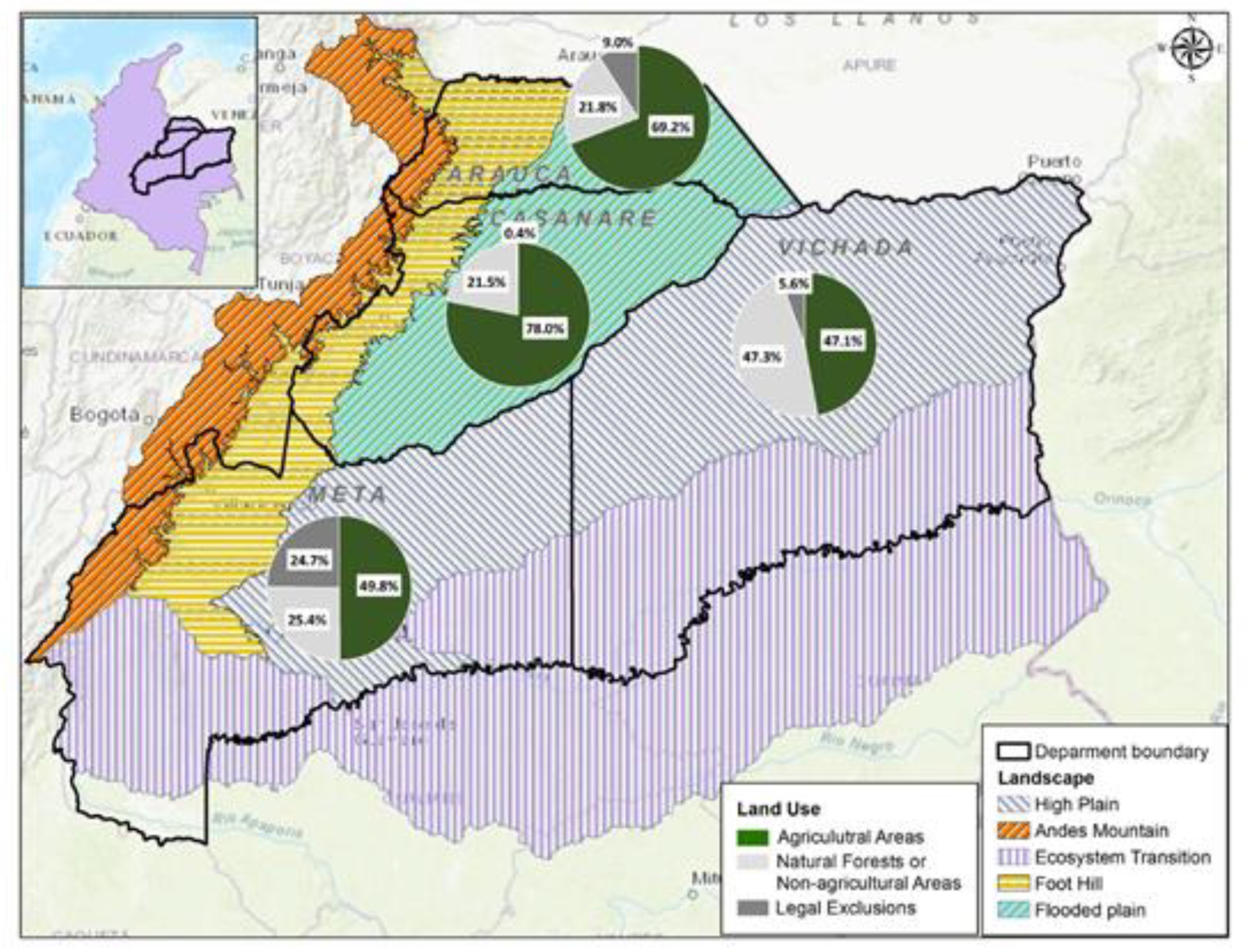
2.1. Study Area

The Orinoquia region of Colombia includes the departments of Arauca, Casanare, Meta, and Vichada. It covers about 25.4 Mha [23] of which about 9.9 Mha (i.e., 39%) are no-go areas for agricultural activities (i.e., natural forest, national parks, indigenous areas, archaeological heritage areas, etc.) [12]. Approximately 15.5 Mha (i.e., 61%) is within the agricultural frontier of which 7 Mha is currently used for agricultural production (i.e., 10% cropland and 90% pastureland) [24] and 8.5 Mha, which consists of flooded savannas and shrubland, is considered to be available for agricultural production [24]. Extensive cattle grazing (0.6 Animal Unit ha⁻¹, where one animal unit is equivalent to 450 kg of average animal-live-weight) [15] occupies around 6.2 Mha [25] and is one of the key economic activities of the region [13,15,26]. About 0.6 Mha is currently used as cropland, where the most dominant crops in terms of cultivated area are oil palm (33%), rice (32%), plantain (14%), corn (10%), soybean (7%), and cassava (3%) [24].

The Orinoquia region includes five subregions, i.e., Andes mountains, foothills, flooded plains, highplain, and an ecosystem transition region (Figure 1). The ecosystem transition region is the transition area between the savannas and the Amazon. Both the ecosystem transition and the Andes mountain region are part of the 9.9 Mha of no-go area for agriculture activities. The flooded plain, foothills, and highplain subregions are within the agricultural frontier and are therefore included in this study. Despite the flooded plain remain flooded most of the year (⁺/₋8 months) [21,27], this area has been used for small-scale extensive cattle production for decades [21]. According to the Rural Agricultural Planning Unit of Colombia (Unidad de Planeación Rural Agropecuaria de Colombia, UPRA), this area has low suitability for crop production but has the potential to continue cattle production [28] in small-scale [21]. The foothills and the high plains subregions hereinafter called “foothills–highplain area” are currently used mostly for large-scale extensive cattle production [10]. This area has the highest potential to increase cattle productivity and generate potential suitable surplus land [13]. The land distribution (in Mha) and land suitability for crop and cattle production of the three subregions are reported in

Table A6. Land distribution and land suitability in the Orinoquia region.

Characteristics	Orinoquia Region
Entire region area a	25.4 Mha
Available agricultural area b	15.5 Mha
Regional landscape	Flooded plain		Foothill		High plain
	5.0 Mha		2.8 Mha		9.7 Mha
Land suitability c within the agricultural frontier	Crops	Cattle	Crops	Cattle	Crops	Cattle
	+	+++	++	++	+++	++

^a Area that covers the limits of four departments Arauca, Casanare, Meta, and Vichada [23]. ^b Official data of the national government which corresponds to available land for agricultural production in the Orinoquia region, Also called Agricultural frontier [23]. ^c According to the zoning of production areas within the agricultural frontier made by [12,28], land suitability is classified as follow: highly suitable (+++) corresponds to land with the best physical, ecosystem and socio-economic conditions for crop or cattle production. Moderately suitable (++) is related to areas with moderate physical, ecosystem or socioeconomic limitations that require investment around the area for optimal production management. Lowly suitable (+) is related to areas with significant limitations (physical, ecosystem or socioeconomic), which require large investments or the development of new technologies for optimal production [12,28].

in the Appendix B.

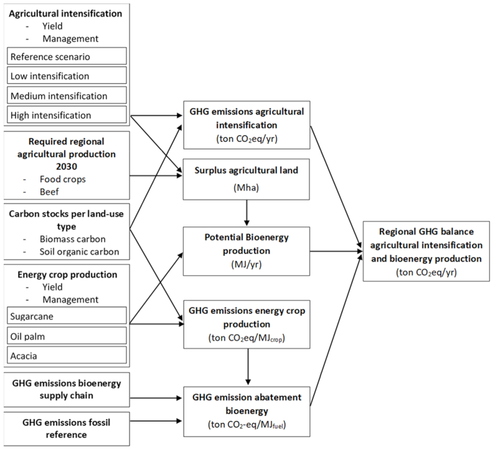
2.2. General Approach

The net GHG balance of the Orinoquia region for 2030 is calculated considering (i) agricultural intensification of food crop and beef production and (ii) bioenergy from energy crops produced on the generated surplus land. We first determine agricultural production for 2030 (Section 2.3). Since most of the crops produced in the region are destined for human consumption, they are referred to as food crops in this study. Moreover, since most of the region’s cattle production is dedicated to beef production, only beef production is included in this study. Next, we assess how agricultural productivity may develop until 2030 and calculate the resulting surplus (or shortage) of land (Section 2.4). Our analysis is conducted for four scenarios; besides a reference scenario, which assumes a business-as-usual development in agricultural intensification, three agricultural intensification scenarios are included (low, medium, high). We then determine GHG emissions for agricultural production and intensification (Section 2.5), for bioenergy supply chains and their reference fossil fuel chains (Section 2.6) and land use change (Section 2.7). Three biomass production routes (i.e., sugarcane bioethanol, palm oil biodiesel, and acacia wood for bioelectricity) are considered, assuming production only takes place on surplus land. Note that each energy crop is analyzed individually, which means, each energy crop is planted on 100% of the land released in each scenario (i.e., only oil palm, or only sugarcane, or only acacia is planted on surplus land by scenario). We do not consider planting the three energy crops at the same time in an area. By combining the GHG emissions of agricultural intensification, bioenergy production, and LUC, the overall GHG balance for the region is estimated for each scenario and each energy crop. Figure 2 presents an overview of the main steps of our approach.

2.3. Agricultural Production in 2030

Food production in the Orinoquia region in 2030 is calculated according to Equation (1). Food production is estimated at national level, multiplying the estimated national population in 2030 with the per capita consumption, the self-sufficiently ratio (SSR) and food losses of each food product. National food production is then multiplied by the contribution of the Orinoquia region to the national production of each food product. The per capita consumption of food products in Colombia is expected to increase towards 2030 [1,30]. In line with the studies of MADR, (2016) and Younis et al., (2020), the SSR, food losses, and the relative contribution of Orinoquia region to national food production are assumed to remain stable to 2030. The land demand projection for agriculture in 2030 is based on the amount of land in use in 2018 (crops and cattle). For input data, see

Table A1. Data inputs for estimation of required food production in the Orinoquia region of Colombia in 2030.

	Per Capita Consumption a (kg/person/year)		SSR b (%)	Food losses b (%)	Contribution c Orinoquia to National Production (%)	Land Use in the Region (ha) 2018 c
	2018	2030
Population Colombia d	48,258,494	55,678,083
Rice	42.2	42.2	90	28	50	176,391
Oil palm (CPO)	33.3	35.0	106	19	40	178,227
Corn	30.2	31.0	33	28	50	57,387
Plantain	53.6	68.0	102	55	30	78,673
Soybean	35.7	37.5	23	19	90	37,340
Cassava	38.5	38.5	99	40	30	18,912
Beef	18.9	24.0	105	22	.	6,239,309

^a Per capita consumption data from [1,17,30,56,57]; ^b Based on data from 17 and 30. SSR relates domestic food production with imports and exports of food products. Thus, SSR values greater than 100% indicate large export quantities while SSR values lower than 100% express large import quantities 17. The projected food consumption is based on assuming that Colombia follows the general trend of Latin America for 2030 30. The SSR, food losses, and the contribution of Orinoquia to national food production is assumed to be the same in 2030 as in 2018. ^c Data from 24. ^d Data from [58].

in the Appendix A.

$$FoodPr{o}_i=Pop\ast Co{n}_i\ast SS{R}_{i }\ast P_{i. orq}\ast \left(100\%+Los{s}_i\right)$$

(1)

where: FoodPro_i = Orinoquia food production (t yr⁻¹); i = Food product (rice, corn, soybean, cassava, plantain, palm oil, and beef); Pop = National population; Con_i = Per capita consumption for food product i (kg person⁻¹ yr⁻¹); SSR_i = Self-sufficiently ratio of food product i (%); P_i.orq = Orinoquia contribution to national production per each food product i (%); Loss_i = Food losses in the supply chain for food product i (%).

After calculating the production per food product for 2030, we calculate the land required for food production in 2030 for each scenario by dividing the production by the yields related to each scenario Equation (2).

$$Land{D}_i=FoodPr{o}_i/Yiel{d}_{i Scenario}$$

(2)

where: LandD_i = Land demand for food production (ha); FoodPro_i = Orinoquia food production (t yr⁻¹); Yield_iscenario= Yield of food product i for each scenario (reference, low, medium, and high) (t ha⁻¹ yr⁻¹).

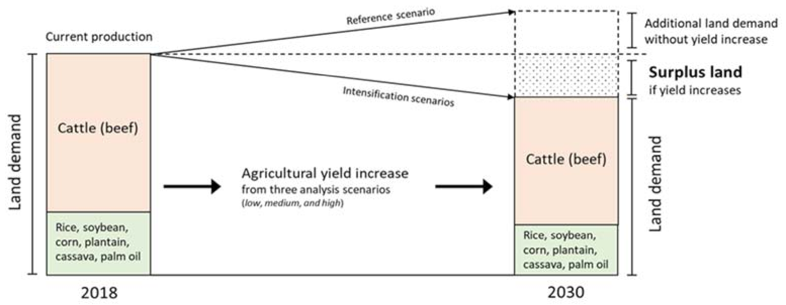
2.4. Agricultural Intensification (Food Crops and Cattle)

Increasing agricultural productivity in the region could generate surplus land if the increase in productivity surpasses the increase in demand for agricultural products. Figure 3 illustrates how surplus land is determined, i.e., the difference between current land demand and future land demand that is projected according to different levels of agricultural intensification (see

Table 1. Yield levels and cattle densities for the reference and agricultural intensification scenarios.

Characteristics		Scenarios 2030				Data Sources
		Reference	Low	Medium	High
Yield food crops (t ha−1 yr−1) a	Rice	4.97	5.06	5.26	5.96	[24,27,41]
	Corn	5.50	6.00	6.00	7.00
	Oilpalm (crude palm oil)	2.41	2.62	2.96	3.30
	Plantain	13.00	16.00	18.00	22.45
	Soybean	2.50	2.53	2.80	3.00
	Cassava	14.00	15.00	18.00	20.74
Livestockproductivity (AU ha−1) b	Cattle	0.6	1.0	1.5	2.0	[15,39]

^a Food crop yields increase are based on historical data analysis of agricultural production for the period 2012–2018 for the whole Orinoquia region. Reference scenario: 50th percentile yield level; Low scenario: 65th percentile yield level; Medium scenario: 80th percentile yield level; High scenario: 95th percentile yield level; ^b AU = animal unit. One AU is equivalent to 450 kg of average animal-live-weight [42].

). The intensification scenarios assume improved agricultural practices such as the efficient use of fertilizers and the reduction of fossil fuel consumption. Before describing the key characteristics of improved agricultural practices and resulting yields below, we first summarize the scenarios here; additional information on the scenarios can be found in Appendix B. The reference scenario follows the conventional agricultural conditions (i.e., inefficient practices in fertilizer application and soil management). For the low intensification scenario, conventional agricultural practices are assumed, with an increase in crop yield based on some improvement in fertilizer application. In the medium intensification scenario, improvement of some agricultural practices is assumed such as crop fertilization and improved cattle management (cattle are fed with improved grasses and forage sorghum). For the high intensification scenario, sustainable intensification is assumed, with fertilizer application in accordance with soil requirements, soil improvements, and improved cattle feed quality (see Appendix B).

2.4.1. Food Crop Production

According to UPRA (2019), current fertilizer use is inadequate in Colombia since the application is not carried out based on soil analysis or plant nutrient requirements. This can result in deficits or excess of fertilizers and affects crop yields [31]. In this study, the fertilizer inputs per scenario, to achieve the crop nutrition requirements, consider the three main nutrients Nitrogen (N), Phosphorus (P), and Potassium (K). The amount of nutrients (kg ha⁻¹) applied to each crop is based on literature and is related to the yield (see

Table A2. Input data for food crops stage in the reference and intensification scenarios.

Scenarios a	Food Crop	Nutrient (kg ha−1)			Diesel Usage (liters t−1) d
		N b	P2O5	K2O
Reference	Rice Corn Oil palm c Plantain Soybean Cassava	110 121 78 47 200 56	36 50 24 6 46 14	157 126 163 65 99 53	25.10 2.73 4.92 8.33 16.20 1.96
Low	Rice Corn Oil palm Plantain Soybean Cassava	140 165 108 72 253 75	46 69 33 10 58 18	200 172 224 100 126 71	24.26 2.64 4.76 8.05 15.66 1.89
Medium	Rice Corn Oil palm Plantain Soybean Cassava	123 143 92 65 240 81	40 59 28 9 55 19	175 148 190 90 119 75	23.45 2.55 4.60 7.78 15.14 1.83
High	Rice Corn Oil palm Plantain Soybean Cassava	138 165 104 90 243 89	45 69 32 12 56 21	196 172 214 125 121 83	22.67 2.46 4.44 7.52 14.63 1.77

^a For all scenarios. fertilization data to each crop were calculated based on data from [63]. ^b The annual amount of synthetic N-fertilizer applied to crops also correspond to F_SN value in Equation (A1) and Equation (A2). ^c For oil palm crop, the amount of fertilizer is expressed per ton of fresh fruit bunches (FFB). ^d Diesel consumption for the reference scenario is based on literature as follow: data for rice taken from [64]; for corn [65]; for oil palm [22]; for plantain [66]; for soybean [67]; for cassava [68]. For the intensification scenarios, it was assumed that diesel consumption would decrease from the reference scenario until reaches a reduction up 10% in the high scenario. This reduction is being considered based on the study by [32].

in the Appendix B). Another important factor in agricultural yield intensification is crop mechanization [5]. Agricultural mechanization in Colombia is used mostly for soil preparation and harvesting, while the other tasks can also be carried out manually [31]. Rice is the crop that uses the most machines/equipment in Colombia [31]. In the Orinoquia region, rice is grown in rainfed conditions (dry rice), which means this crop receives water mainly from rainwater. Therefore, it does not require mechanization linked to irrigation [31]. Although currently mechanization is used in agriculture, there is not enough available historical data about fossil fuel consumption related to each crop in Colombia. Therefore, diesel usage in the reference scenario is based on literature as shown in Table A2 in the Appendix B. For the intensification scenarios, diesel consumption was assumed to reduce by 10% in the high scenario compared to the reference scenario, based on the study by Brinkman et al. (2018) [32] (see Table A2 in the Appendix B).

To establish the crop yield levels for each scenario, data analysis of agricultural yields for the period 2012–2018 for the Orinoquia region was conducted. The yield levels in the reference scenario are set at the 50th percentile of the reported yield levels in Orinoquia region in the period 2012–2018. The low scenario is set at 65th percentile, the medium scenario is set at 80th percentile, and the high scenario is set at the 95th percentile of the yield levels of the Orinoquia region in the period 2012–2018. Thus, for example, the rice crop yield is 4.97 t ha⁻¹ yr⁻¹ for the reference scenario and for the intensification scenarios, crop yields are 5.06; 5.26; and 5.96 t ha⁻¹ yr⁻¹ for the low, medium, and high scenarios, respectively. Projected yields for all food crops are shown in Table 1.

2.4.2. Beef Production

To increase cattle productivity, the production system can be intensified by several improvements such as fertilizing pastures, improved grasses, a better quality of animal feed, and pasture rotation [21,33,34,35,36]. The current cattle production in the region is carried out in an extensive system. Considering that in this system (i) the pastures do not receive fertilization at any time of their lifetime, and (ii) the soil of the region is low in nutrients [37], we assume that the land from current cattle production is degraded. Since all future scenarios include cattle production on the current degraded land, we assume that in all future scenarios the land used for cattle is degraded. However, as better practices are applied to increase productivity, the increase in beef yield includes the improvement of cattle production systems with the use of improved (fertilized) pastures and silvopastoral systems as described as follow.

For the reference and low scenario, the current extensive production system of the foothill-high plain area is assumed, in which animal feed is based on pastures with low nutrient levels (e.g., Trachypogon vestitus) [10,37,38]. For the medium and high scenarios, it is assumed the cattle feed quality is improved (see Appendix B), using improved grassland (e.g., Brachiaria decumbens) and forage sorghum for the medium scenario [29]. While a mix of improved grassland (e.g., Brachiaria decumbens), fodder plants (e.g., leguminous herbs, and shrubs/trees), and forage sorghum improve the quality of the animal feed in the high scenario (it has been considered that for sustainable development of cattle production, the use of a silvopastoral grazing system is proper [33]). It was considered that the sorghum forage needs to be cultivated within the land used for cattle production. This land use is included in the total GHG emissions for cattle production as feed emissions. The characteristics of the production systems for the reference and intensification scenarios are described in the Appendix B. The projected increases in cattle productivity for the intensification scenarios follow the three levels of projected productivity increases of the Colombian livestock strategic plan of the National Federation of Breeders [15,39]. We consider these projected increases in cattle productivity realistic given the large range in current productivity, wherein some traditional farms an animal density of 1.5–1.8 heads per hectare is achieved. while in farms with improved systems animal densities of 3–4 heads per hectare are realized [40]. The resulting yields are reported in Table 1.

2.5. GHG Emission Associated with Agricultural Production

The GHG emissions of agricultural production were calculated for each scenario, taking a system boundary of cradle-to-farm gate. The emissions for all crop systems are expressed as kg CO₂eq t⁻¹ of product, which corresponds to tons of rice, tons of corn, tons of soybean, tons of plantain, tons of cassava, and tons of oil palm-fresh fruit bunches. For beef production, the emissions are expressed as kg CO₂eq t⁻¹ beef. The emissions include LUC-related emissions (see Section 2.7) and the emissions related to (annual and perennial) crop cultivation and beef production. The GHG emissions related to crop production include emissions of fertilizer production, fertilizer application, and diesel usage. In addition, since one of the annual crops is rice, methane (CH₄) emissions from rice production are included following the Equations (A3) and (A4) in the Appendix B. The fertilizer application rate is related to the yield and the nutrition requirements of each crop, see Table A2 in the Appendix B. For example, it was assumed that in a sustainable scenario like our high scenario, the fertilizer is applied according to the soil requirements. Furthermore, to improve the fertilization of crops, we assumed an increase in the efficiency of the use of nitrogen fertilizers that includes both the use of good agricultural practices and the use of slow-release nitrogen fertilizers (Appendix B). Emissions from fertilization include fertilizer production and direct/indirect N₂O emissions of fertilizer application. For the diesel usage, we assumed the fossil fuel use by machinery goes down with higher agricultural yields, due to higher efficiency of the agricultural operations per ton of output. Diesel usage per crop per scenario, emission factors of fertilizers, and fertilizer application are included in Table A2 and

Table A3. Emission factors for all type of crops (food, energy, and feed) in the cultivation stage in the reference and intensification scenarios.

• Fertilizers production emission factors:	Unit	EF
Urea as N (0.46% N) a	kg CO2eq/kg Fertilizer	3.38
Ammonium sulphate (SAM) as N (0.21% N) a		2.79
Diammonium phosphate (DAP) as P2O5 a		1.61
Potassium chloride as K2O a		0.53
Triple super phosphate (TSP) b		0.34
Controlled release nitrogen fertilizer as N (0.46% N) c		2.79
• Field N2O emission factors d
FSN (annual amount of synthetic N-fertilizer applied)	kg N ha−1	correspond to values listed in the column for N-nutrient
FracGASF (fraction of synthetic fertilizer N that volatilizes as NH3 and NOX)	kg N volatilized (kg of N applied)−1	0.11
FracLEACH (fraction of all N added to/mineralized in managed soils in regions where leaching/runoff occurs that is lost through leaching and runoff	kg N (kg of N additions)−1	0.24
EF1	kg N2O–N (kg N)−1	0.01
EF4	kg N2O–N (kg NH3–N + NOX–N volatilized)−1	0.01
EF5	kg N2O–N (kg N leaching/runoff)−1	0.011
• Fossil fuel emission factors e
Diesel production	kg CO2/kg diesel	0.569
Burning diesel	kg CO2/kg diesel	3.188
	kg CH4/kg diesel	0.00045
	kg N2O/kg diesel	0.00008

^a Emission factors for fertilization production are taken from Ecoinvent database, version 3.0.1.0. ^b Data from [64]. ^c Controlled release nitrogen fertilizer as N (0.46% N), was assumed to report a lower production emission factor compared to Urea. Therefore, the emission factor of the lowest nitrogen fertilizers (SAM) is applied. ^d Emission factors for N₂O emissions calculation (direct/indirect) resulting from N-fertilization were taken from [43]. ^e Fossil fuel emission factor were taken from [43].

in the Appendix B.

The GHG emissions from beef production includes emissions from feed production (CO₂ and direct/indirect N₂O; these emissions are calculated as for food crops), enteric fermentation (CH₄), and manure management (CH₄ and direct/indirect N₂O). Emissions were calculated following IPCC 2019 Refinement guidelines (i.e., equations: 10.21; 10.22; 10.30; 11.1; and 11.5) [43]. Note that for all scenarios in this study, it is estimated that all cattle production is run on a grazing system. Therefore, following the IPCC 2019 method, it corresponds to the manure management system PRP i.e., “Pasture/Range/Paddock” where manure is not managed [43]. We assumed the increase in beef productivity is related to better quality/quantity feed supply (dry matter intake). This is because the change from pastures with low nutrient levels to pastures which deliver a higher nutrient content via the integrated systems of trees and fodder. This better fodder improves the digestibility of dry matter and increase the nutritional value of the feed, in terms of total protein and minerals [33,44].

Moreover, sustainable cattle production also includes better animal welfare (disease management), better management of pastures, fodders, and soil quality. One of the sustainable cattle production systems suggested for Colombia is called the silvopastoral system which could contribute to improving soil conditions and increasing C-stock [13,33]. The input data for calculating the GHG emissions of beef production for all scenarios are included in

Table A4. Input values for the calculation of GHG emissions of beef production in the reference and intensification scenarios.

Input Data	Unit	Scenarios 2030
		Reference	Low p	Medium q	High q
Animal density a	AU ha−1	0.6	1.0	1.5	2.0
Animal population b	heads of cattle	9,331,160	9,064,783	8,317,333	7,110,636
Subcategories of cattle c
Growing cattle	heads	1,662,006	1,614,561	1,481,430	1,266,501
Other mature cattle (beef)	heads	2,638,502	2,563,181	2,351,830	2,010,621
Mature double-purpose cattle	heads	5,030,652	4,887,042	4,484,074	3,833,515
Beef extraction factor d	%	52.5	52.5	53.0	53.0
Extraction rate e	%	17.5	17.5	18.2	20.0
TAM (typical animal weight) a
Growing cattle	kg animal−1	144	144	200	220
Other mature cattle	kg animal−1	350	380	425	485
Mature double-purpose cattle	kg animal−1	380	383	388	399
Total daily dry matter intake (DMI)f
Growing cattle	kg day−1 animal−1	4.7	4.7	6.2	6.5
Other mature cattle		8.6	9.0	9.7	10.5
Mature double-purpose cattle		8.8	8.8	8.9	9.1
Data for feed intake estimates
Estimated dietary net energy concentration of the feed (Nemf) g	MJ kg−1 dry matter−1	4.5	4.5	6.0	7.0
Gross energy intake (GE) h
Growing cattle	MJ kg−1 dry matter	86.4	86.4	114.0	119.8
Other mature cattle		159.3	166.9	178.3	193.5
Mature double-purpose cattle		162.1	162.9	164.3	167.3
Methane (CH4) emissions from enteric fermentation
CH4 conversion factor (Ym) i	%	7	7	6.3	6.3
Methane (CH4) emissions from manure management
Volatile Solid excretion rate j (VST,P)	kg vs. (1000 kg animal mass)−1 day−1	8.6	8.6	8.5	8.1
Fraction of total annual vs. for each livestock species/category T that is managed in manure management system S in the country, for productivity system P, animal waste management systems (AWMS) k	Dimensionless	0.92	0.92	0.92	0.92
Emission factor for direct CH4 (EF) l	g CH4 kg VS−1	0.6	0.6	0.6	0.6
N2O emissions from manure management
Nitrogen excretion rate (Nrate) m	kg N (1000 kg animal mass)−1 day−1	0.29	0.29	0.31	0.36
Annual N excretion (Nex) n
Growing cattle	kg N animal−1 yr−1	15.24	15.24	22.63	28.91
Other mature cattle		37.05	40.22	48.09	63.73
Mature double-purpose cattle		40.22	40.54	43.90	52.43
EF3 to estimate direct N2O emissions from managed soils o	kg N2O-N (kg N)−1	0.006	0.006	0.006	0.006

^a Data from [15,39]. ^b Animal population data was calculated considering the beef requirement per year, animal unit per ha, beef extraction factor, and extraction rate per scenario. ^c The cattle population was classified into three main subcategories according to [43] and it was considered the share for each category according to the information taken from [57]. ^d It is the percentage of carcass beef with respect to the live animal’s weight. Data from [39,57]. ^e It correspond to the percentage of the annual quantity of slaughtered beef cattle, Data from [39,57]. ^f Own calculations based on the animal live-weight per categories and its relationship with the daily dry matter intake. ^g Considering that in Table 10.8a in chapter 10 of IPCC, 2019, the diet quality can be selected, we assumed low quality diet in the reference and low scenario. Moderate quality diet for medium scenario and high-quality diet for the high scenario. Then, average default values from Table 10.8a are selected [43]. ^h GE was calculated by multiplying the DMI value by the default value of 18,45 MJ kg⁻¹ of dry matter [43]. ⁱ The Ym value of 7.0 is apply in reference and low scenario assuming non-dairy animal category and the non-feedlot diets (low quality pasture). The Ym value of 6.3 is apply in the medium and high scenario assuming high quality forage diets [43]. ^j Default values for volatile solid excretion rate from Table 10.13A of the chapter 10 for Latin America region from [43]. For the reference and low scenario, it was selected “low PS for other cattle.” For the medium scenario, it was selected “means value for other cattle”. For the high scenario, it was selected “High PS for other cattle”. ^k Default values in chapter 10 from [43]. ^l Default values in chapter 10 from [43]. Methane emission factor for all animals in low and high productivity under a pasture, range, and paddock manure managed system. ^m Default values from Table 10.19 of the chapter 10 for Latin America region from [43]. For the reference and low scenario, it was selected “low PS for other cattle”. For the medium scenario, it was selected “means value for other cattle”. For the high scenario, it was selected “High PS for other cattle”. ⁿ Calculated with Equation 10,30 [43]. ^o Default value for wet climates from Table 11,1 in chapter 11 from [43].

in the Appendix B. Considering that the IPCC 2019 methodology refined some of the default data according to high and low cattle productivity systems [43], we assume the use of these default data (when available) to apply it to the scenarios according to the related best practices (see Table A4 in the Appendix B).

2.6. GHG Emission Associated with Energy Crops

It is assumed that energy crops are cultivated, one at a time, on the surplus land obtained from the agricultural intensification described in Section 2.4. The amount of energy crops that can be produced depends on the amount of surplus land generated in each scenario and the energy crop yield (see

Table A7. Data and assumptions for emissions of energy crops. These crops only grow in surplus land from the medium and high scenarios of agricultural yield increase.

Input Data			Scenarios by 2030
			Medium	High
Crop yield (t ha−1 yr−1) (wet basis)	Sugarcane a		84.3	85.4
	Oil palm b		16.6	18.4
	Acacia c		16.5	19.3
Fertilization d (kg ha−1)	Sugarcane	N	48	49
		P	114	116
		K	116	118
	Oil palm	N	92	104
		P	28	32
		K	190	214
	Acacia	N	109	127
		P	99	116
		K	52	61
Diesel consumption e (l t−1)	Sugarcane		3.38	3.27
	Oil palm		4.60	4.44
	Acacia		3.84	3.71

^a Yield data from [24,41]. Sugarcane is expressed in tons of cane per hectare. Note sugarcane crop yield does not report great variation between scenarios because the data were taken from the only current crop in the region with information from 2013–2018. Where medium scenario corresponds to percentile 80 of the period data; and high scenario corresponds to percentile 95. ^b Yield data from [77]. Oil palm yield is expressed in terms of Fresh fruit bunches (FFB) per hectare. The yield increase follows the regional data for the period 2012–2018. Where medium scenario corresponds to percentile 80 of the period data; and high scenario corresponds to percentile 95. ^c Yield data from [78] Acacia is expressed in tons of wood per hectare. ^d For all scenarios, fertilization data to each energy crop were calculated based on data from [63]. The use of nitrogen fertilizers has implications for GHG emissions as described in Appendix A. ^e Diesel consumption for oil palm is based on data from [22]. Diesel consumption in sugarcane from [79]. Diesel consumption in acacia plantation is taken from a forest harvesting system working the traditional forestry tasks using chainsaw, winch, and walking tractor [80].

in the Appendix C). Since only in the medium and high scenarios large amounts of surplus land are obtained, energy crop cultivation is only evaluated for these two scenarios. The GHG emissions of energy crops include the emissions related to cultivation (fertilization and fossil fuel consumption) and to LUC. Emissions from fertilization include fertilizer production and direct/indirect N₂O emissions of fertilizer application (Table A7). The calculation of the GHG emissions of energy crop cultivation follow the same logic as for food crops, see Section 2.5. In Table A3 and Table A7 of the Appendix B and Appendix C, all input data and factor emissions for the calculations of the GHG emissions of energy crops cultivation are included.

2.7. GHG Emission Related to Land Use Change

The expansion and contraction of agricultural land and the use of surplus land for energy crops results in changes in C-stock. Changes in C-stock were calculated for five different possibilities of LUC in the Orinoquia region as follows: considering that for the reference and low scenarios, the increase in agricultural land demand requires the use of natural vegetation (shrubland) and that forest is excluded for agricultural land use, the land-use conversions for these two scenarios are (a) from shrubland to cropland for food crops production. (b) From shrubland to pastureland in degraded pastures for cattle production (i.e., pastures with low nutrient levels). Note that in line with Rincon Castillo et al., (2012) and Rodríguez Borray et al., (2019), we assume that the land currently used for extensive cattle production is degraded. Therefore, the considered land-use conversions in the medium and high intensification scenarios are (c) cropland to cropland for food crops and (d) from degraded pastures to managed pastures for cattle production (beef). In the intensification scenarios, all the surplus land comes from cattle production areas (i.e., pastures with low nutrient levels). Therefore, for energy crops production the considered land use conversion is (e) from degraded pasture to energy crops (sugarcane, oil palm, and acacia). GHG emissions caused by changes in C-stocks due to the LUC food crops were calculated using Equation (3).

$$\begin{gathered} {\mathrm{E}}_{\mathrm{LULUC}}=\Delta CS\ast 44/12\ast 1/20\ast 1/P \\ {\mathrm{E}}_{\mathrm{LULUC}}=\left(C{S}_R\ast 44/12\ast 1/20\ast 1/P\right)-\left(C{S}_A*44/12*1/20*1/P\right) \end{gathered}$$

(3)

where, E_LULUC = GHG emissions from C-stock change due to LUC (t CO₂eq t⁻¹ crop product). ΔCS = CS_R − CS_A (CS_R = C-stock associated with the prior land-use (t C ha⁻¹); CS_A = C-stock associated with the new land-use (t C ha⁻¹). P = crop productivity (t ha⁻¹ year⁻¹). An amortization period of 20 years is assumed. The factor 44/12 is used to convert carbon into CO₂.

Each land use has a different carbon stock. The total C-stocks, including above and below ground biomass and SOC, of each land use type are included in

Table 2. Carbon stock including above and below ground biomass and SOC for various land use types in the Orinoquia region based on Castanheira et al., (2014), unless otherwise specified.

Land Use Type	Total Carbon Stock (t C ha−1)
Cropland	33
Shrubland	126
Degraded pastures for cattle production	50
Managed pastures for cattle production (medium/high scenario)	86/105
Oil palm (low/medium/high scenario) a	113/121/129
Sugarcane (medium/high scenario) b	62/65
Acacia (medium/high scenario) c	85/90

Note that in this study, energy crops are only planted in surplus land of the medium and high scenario. The C-stock for energy crops in the medium scenario corresponds to the average between the C-stock of the low and the high scenario. ^a Data for low scenario from [45]. Note that in this study, oil palm is used both as a food crop and as an energy crop. ^b High C-stock value from [46]. The low C-stock value (59.3) taken from [47]. ^c Data from [48]. The low C-stock value corresponds to 80 t C ha⁻¹.

. The time to be considered for changes in C-stocks was 20 years, in line with [43].

2.8. Total GHG of Bioenergy Supply Chains

The total GHG emissions of sugarcane-bioethanol, palm oil-biodiesel, and acacia-bioelectricity include GHG emissions of energy crop cultivation, LUC, conversion plant (industrial production stage), and combustion (i.e., it refers to the conversion of biofuel to heat, electrical, or mechanical energy). For this study, it is assumed that the conversion plant for each bioenergy chain includes the following stages:

• For bioethanol, conversion plant includes cane transport, milling process, and ethanol plant [49].
• For biodiesel, conversion plant includes palm oil mill, physical refining (refined, blanched, and deodorized); transesterification; esterification of the free fatty acid (FFA); BD purification; glycerin purification (USP), and methanol recovery [22].
• For bioelectricity, conversion plant includes sawmill and pellet mill [50]. It was assumed a CHP (combined heat and power) system for bioelectricity production. For the calculation, the stationary combustion emissions factor of the IPCC, 2019 (volume 2, chapter 2) was used.

Data and emission factors in the three-supply chain are presented in

Table A8. Data of emissions along the production process of sugarcane-ethanol, oil palm-biodiesel and acacia-bioelectricity production.

Emissions	Unit	Bioethanol		Biodiesel		Electricity
		M	H	M	H	M	H
Cultivation emissions a	kg CO2eq t−1biofuel	−39.0	−143.0	−3089.0	−3207.4
	kg CO2eq MJ−1electricity					−0.071	−0.084
Conversion plant	kg CO2eq t−1biofuel	6.4 b		145.5 c		0.0114 g
Combustion	g CO2eq MJ−1biofuel	0.3 d		0.3 d
	g CO2eq MJ−1electricity					1.9 e
Fossil fuel comparator f	g CO2eq MJ−1biofuel	94		94
	g CO2eq MJ−1electricity					183
Total emissions	g CO2eq MJ−1biofuel	−2.1	−6.0	−79.3	−82.5
	g CO2eq MJ−1electricity					−68.9	−82.1

^a Data from energy crop production in the medium (M) and high (H) scenarios of the present study. ^b Data from [49]. ^c Data from [22]. ^d Data calculated based on Tier 1, [43]. It includes CH₄ and N₂O emissions. ^e Data calculated based on Tier 1, [43]. It includes CH₄ and N₂O emissions.Biogenic CO₂ emissions are not considered. ^f Data from [2]. ^g Data from [50].

of the Appendix D. Note that for all three bioenergy supply chains, it was assumed that both the emissions in the conversion plant and the emissions from bioenergy use (combustion) do not vary in the scenarios, since the focus of this study is on the cultivation stage. Emissions from biomass combustion include emissions of methane (CH₄), and nitrous oxide (N₂O), but the biogenic CO₂ emissions of the crop biomass are considered carbon neutral.

The GHG emissions caused by changes in C-stocks due to the LUC energy crops were calculated using Equation (3). The net GHG emissions of the supply chain per bioenergy are calculated using Equation (4).

$${\mathrm{Net}}_{\mathrm{GHG}}={\mathrm{F}}_{\mathrm{C}}+\mathrm{LUC}+\mathrm{CCS}+\mathrm{F}+{\mathrm{B}}_{\mathrm{PE}}+{\mathrm{B}}_{\mathrm{U}}$$

(4)

where, F_C: Fossil fuel consumption emissions. LUC: Land use change emissions. CCS: Crops C-stock sequestration. F: Fertilizer emissions (production and application). B_PE: Bioenergy emissions by industrial production stage, B_U: Bioenergy emissions by use (combustion/burning).

Comparing the GHG emissions of the bioenergy production routes with the emissions from the fossil reference systems (gasoline, diesel, and coal; see Table A8 of the in Appendix D), we evaluate the potential emission savings from bioenergy. Consequently, it is analyzed if the bioenergy GHG reduction levels meet the RED II GHG saving requirements.

3. Results

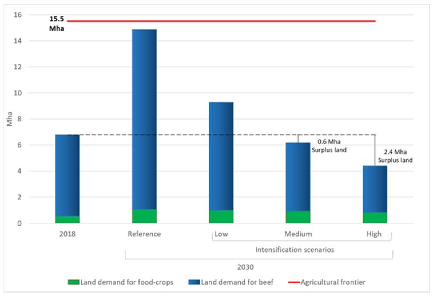
3.1. Agricultural Intensification

In the reference scenario, the total calculated land demand for food production in the Orinoquia region in 2030 is 13.8 Mha, of which about 90% is used for beef production in extensive cattle grazing system (Figure 4). Although this is still within the agricultural frontier area of 15.5 Mha, it is a little more than double the area currently in use for agriculture (6.8 Mha), due to the projected increase in demand. Compared to the reference scenario, there is 38% decrease in agricultural land use in the low scenario, 58% decrease in the medium scenario, and 70% decrease in the high scenario. In the medium and high scenario, the land for cattle production includes the land used to produce forage sorghum for improved beef production (491 and 496 thousand hectares, respectively).

In none of the intensification scenarios was surplus land obtained from food crops. Obtaining surplus land from agricultural intensification is only possible due to improvements in cattle productivity. In the low intensification scenario, there is not surplus land. In the medium scenario, it is possible to obtain 0.6 Mha of surplus land. In the high scenario, about 2.4 Mha of surplus land becomes available, which corresponds to 39% of the area currently used for cattle grazing (i.e., 6.2 Mha).

For the medium and high scenario, the amount of energy cops and bioenergy that can be produced on surplus land is presented in

Table 3. Energy crop and bioenergy potential on surplus land in Orinoquia region in 2030 according for the medium and high intensification scenario.

		Medium Scenario	High Scenario
Sugarcane	Mt sugarcane yr-1	52	201
Bioethanol	PJ yr-1	96	368
Oil Palm	Mt FFB yr-1	10	44
Biodiesel	PJ yr-1	82	349
Acacia	Mt wood yr-1	10	46
Bioelectricity	PJ yr-1	36	162

. The highest bioenergy potentials are obtained when the surplus land is used to produce bioethanol from sugarcane or biodiesel from oil palm. This is due to the relatively higher ratio in the assumed conversion efficiency (MJ biofuel per kg raw material) of sugarcane and oil palm compared to acacia (i.e., one ton of FFB of oil palm produces 0.22 t of biodiesel with a calorific value of 37,000 MJ t⁻¹ _biodiesel, while one ton of sugarcane produces 0.07 t of bioethanol with a calorific value of 27,000 MJ t⁻¹ _bioethanol). In the high scenario, bioenergy potential is 3.8 to 5.4 times higher than in the medium scenario due to higher land availability and higher yield levels of the energy crops.

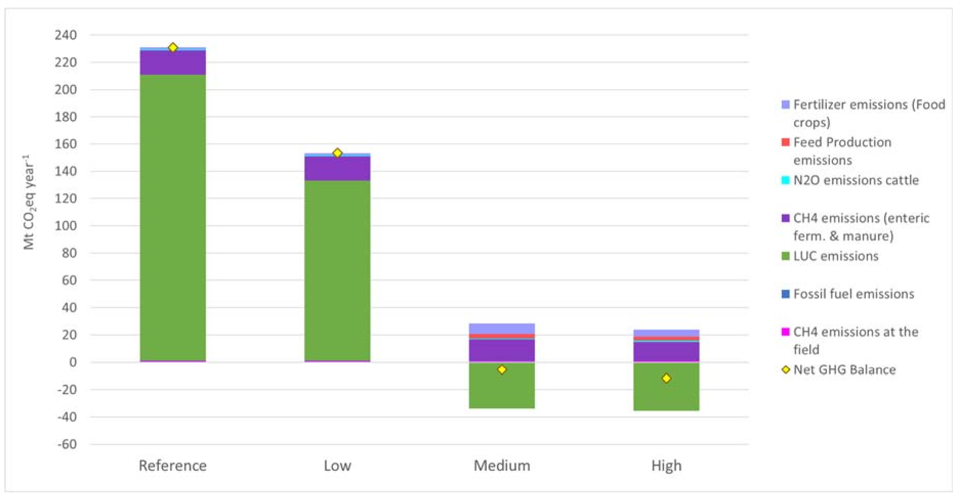
3.2. GHG Emissions Associated with Agricultural Intensification

Figure 5 shows the annual GHG emissions of agricultural intensification (food crops and cattle) for all scenarios in 2030. LUC emissions result from the changes in C-stock due to land use change. The “LUC emissions” value in the figure considers both LUC emissions and C-stocks from food crops and pasture production for cattle. In the reference scenario, the largest GHG emission source is LUC which represents about 90% of the total GHG emissions of agricultural production (food crops and beef). The expansion of beef production is the main cause of LUC-related emissions (318 Mt CO₂eq yr⁻¹) due to the conversion of shrubland to degraded pastures (i.e., pastures with low nutrient levels). Regarding food crops in the reference scenario, the highest contribution to LUC emissions is related to the expansion of rice and oil palm (8.9 and 5.8 Mt CO₂eq yr⁻¹, respectively) due to the conversion of shrubland to cropland.

In the agricultural intensification scenarios, the LUC-related emissions are lower than in the reference scenario, but the low intensification scenario required the conversion of shrubland to degraded pastures to meet the demand for beef. Therefore, the LUC-related emissions in the low scenario are much higher than for the medium and high scenarios (191; 48; and 33 Mt CO₂eq yr⁻¹, respectively). For the medium and high scenario, no natural land is converted to agricultural land and degraded pastures are improved to managed pastures. Moreover, the carbon storage in the managed pastures (fertilized) will increase productivity and therefore also increase the C-stocks of those lands. The emissions of feed production, i.e., sorghum forage, is only reported for the medium and high scenarios (3.4 and 2.9 Mt CO₂eq yr⁻¹, respectively), as in these scenarios it is assumed that the quality of the animal feed was improved. These feed emissions include all emissions related to growing sorghum forage.

Note that, in agricultural production scenarios, the only two crops that report net carbon storage are oil palm and pastures. The oil palm cultivation to produce oil for human consumption is the only food crop that reports a net carbon sequestration as a perennial crop (i.e., negative LUC emissions) since the C-stock value considers the biomass of fronds, trunk and roots, the cover vegetation, and the associated organic matter that remains in the plantation after the harvest of the fruit (FFB). In the case of pastures to produce beef, the yield of beef production is directly linked with higher consumption of grass by cattle. For example, in the high scenario, total grass consumption is higher than in the reference scenario, but the demand for land to produce pastures is less in the high scenario compared to the reference scenario.

In the low, medium, and high scenario, the total (positive) emissions associated with food crop production (fertilization, fossil fuel, and CH₄ emissions at the field) and beef production (CH₄ emissions of enteric fermentation and manure, N₂O emissions) are lower compared to the reference scenario. For the medium and high scenario, the reduction of emission is a result of better management practices such as increasing the fertilizer efficiency, reducing the consumption of fossil fuels, and improving cattle feed quality. Regarding the efficiency of fertilizers, from the application of urea in the reference scenario, we move on to the application of more efficient sources of fertilizer to reduce NH₃ and N₂O emissions by application and volatilization of fertilizers as described in the Appendix B. Regarding fossil fuel, the emission reduction is given mainly by the diesel reduction used by machinery (i.e., higher efficiency).

Regarding cattle feed quality, it is observed that with no change in quality animal feeding, as the number of animals increases, the CH₄ emissions from enteric fermentation could increase, as observed between the current situation (2018) and the reference scenario (10.7 and 17.7 Mt CO₂eq yr⁻¹, respectively). However, with a better-quality feed, the number of animals and their CH₄ emissions by enteric fermentation would be reduced while the animal-beef ratio would be increased, as observed in the medium and high scenario (15.3 and 13.7 Mt CO₂eq yr-1, respectively). When agricultural production intensifies sustainably (i.e., high scenario), there is a reduction in positive emissions of 83% compared to the reference scenario.

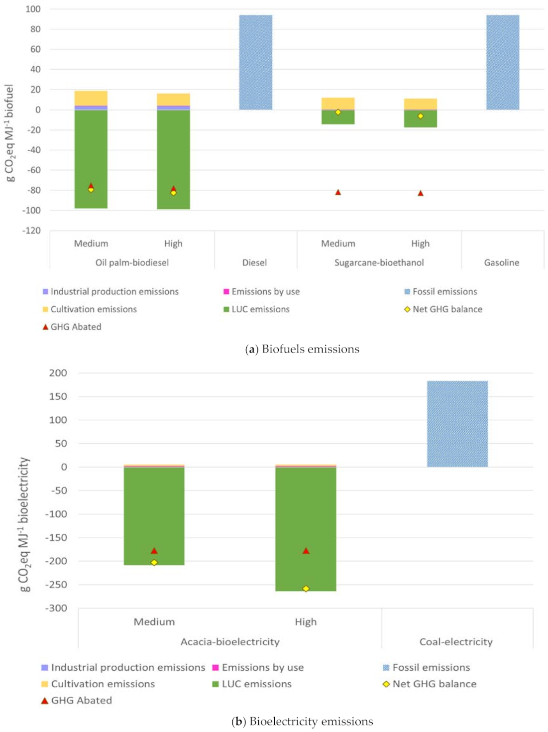
3.3. GHG Emissions Associated with Bioenergy Production

The net GHG emissions of bioenergy production and abated emissions compared to their fossil fuel equivalent for the medium and high scenario in 2030 are shown in Figure 6. For all bioenergy supply chains, the net GHG emissions are slightly higher in the high scenario than in the medium scenario, due to the use of better agricultural practices in the cultivation stage. For all bioenergy supply chains, the GHG emissions related to LUC dominate the GHG balance. Negative LUC emissions (sequestration) vary among bioenergy supply chains because the tree energy crops store much more carbon than the original vegetation present today (i.e., pastures with low nutrients). The LUC emissions from the oil palm crop behave the same as those described in Section 3.2, agricultural intensification.

For both scenarios, the emissions in the conversion of biomass to energy carriers of the three bioenergy chains are lower than the cultivation emissions, as shown in

Table 4. Emissions of bioenergy production for the medium and high intensification scenario.

			Medium Scenario	High Scenario
Sugarcane	Cultivation stage	g CO2eq MJ−1 biofuel	11.7	10.9
	Industrial stage	g CO2eq MJ−1 biofuel	0.2	0.2
Oil Palm	Cultivation stage	g CO2eq MJ−1 biofuel	14.6	12.0
	Industrial stage	g CO2eq MJ−1 biofuel	3.9	3.9
Acacia	Cultivation stage	g CO2eq MJ−1 bioelectricity	27.6	23.9
	Industrial stage	g CO2eq MJ−1 bioelectricity	0.0007	0.0007

. The emissions from the use of biofuels (i.e., N₂O and CH₄ emissions by combustion) are the same for both biodiesel and bioethanol (0.3 g CO₂eq MJ⁻¹ biofuel) and higher for bioelectricity (i.e., burning of acacia pellets) (1.9 g CO₂eq MJ⁻¹ bioelectricity). Logically, under the high scenario, more surplus land is available for bioenergy production than in the medium scenario (2.4 and 0.6 Mha, respectively) and subsequently, the emissions related to each energy crop production system are in line with the quantity of raw material produced (PJ bioenergy yr⁻¹). For example, the high scenario with biodiesel production reports a higher net GHG balance (−82.5 g CO₂eq MJ⁻¹ biofuel) than the high scenario with bioethanol production (−6 g CO₂eq MJ⁻¹ biofuel) as shown in Figure 6a.

The total GHG emissions of biofuels and bioelectricity production, including the emissions related to LUC, cultivation (fertilization and diesel use), conversion and direct use, are compared to their fossil counterpart to calculate the abated emissions (Figure 6). Bioethanol, biodiesel, and bioelectricity production achieve more than 100% emission reduction compared to their fossil fuel equivalent. They thereby meet the RED II GHG saving requirements, which is 65% for biofuels (i.e., bioethanol and biodiesel) and 70% for bioelectricity.

In this study, the emissions resulting from the combustion biofuels in vehicle engines are not calculated, since CH₄ and N₂O emissions are highly dependent on the efficiency of the source technology, emission control, and combustion system that is not the core of this study. However, to identify whether the abated emission could be affected by the combustion of the biodiesel in an engine, we applied the brake thermal efficiency (BTE) of the computerized diesel engine reported by Soly et al. (2021), to the emissions from the biodiesel chain reported in our study (BTE is defined as the ratio of brake power of an engine and the energy of the fuel released during the combustion process [51]. Soly et al. (2021) found a BTE of 25.3% for diesel and 25.6% for biodiesel). As a result, the calculated abated emissions by the use of biodiesel, reported in our study, are affected by up to 1.3%.

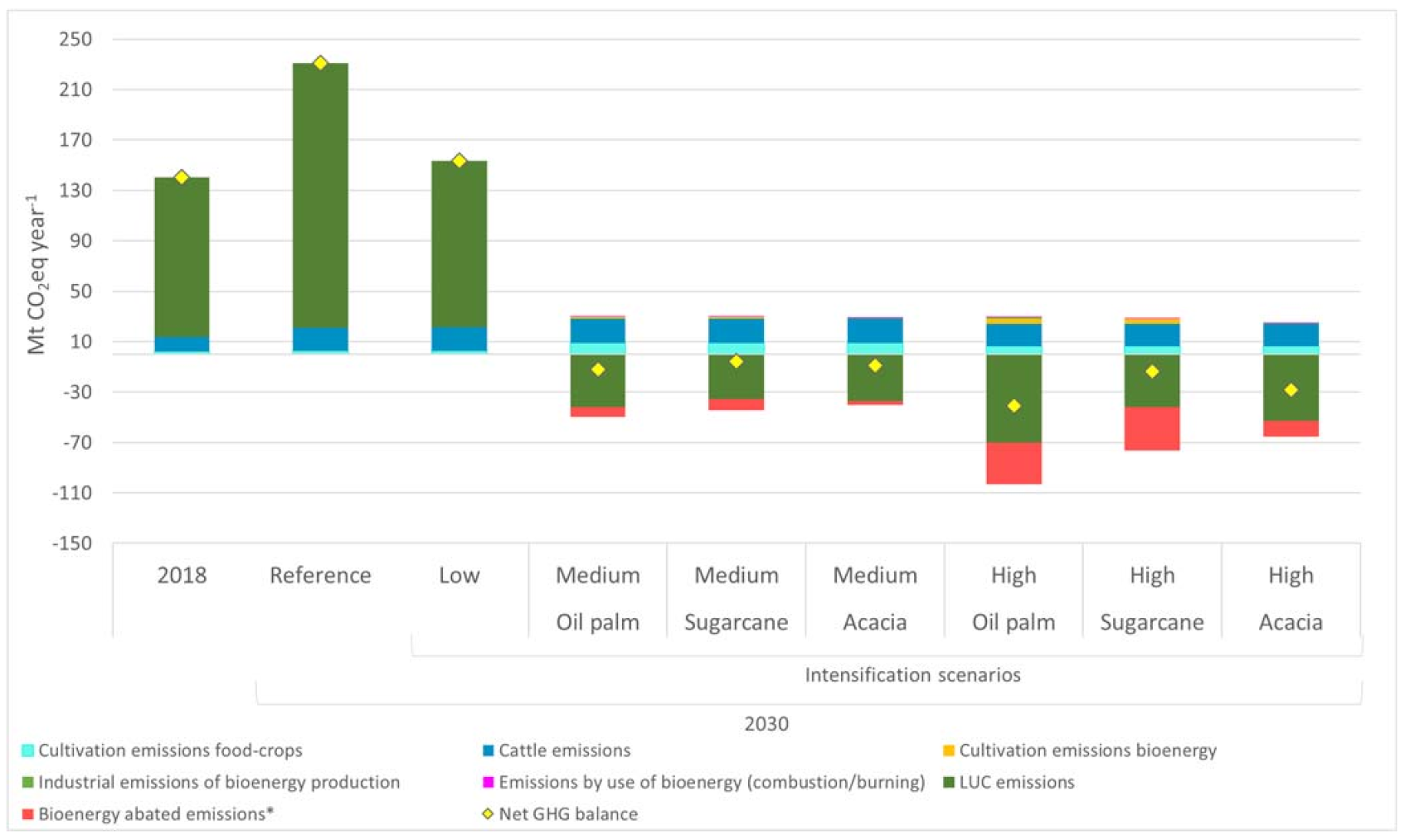
3.4. Regional GHG Balance of Agricultural Intensification & Bioenergy Production

The GHG balance on the entire regional level, for both the agricultural intensification and bioenergy production, is shown in Figure 7. Increased agricultural yields, use of better agricultural practices, and use of surplus land for bioenergy production result in a decrease in net GHG emissions in the medium and high scenario compared to the reference and low scenario, and the current situation (2018). When comparing the net emissions of the reference and low scenario with the emissions of the current situation (2018), the emissions of the low scenario are slightly higher than in 2018 (153 and 141 Mt CO2eq yr⁻¹, respectively). However, the emissions of the reference scenario (231 Mt CO2eq yr⁻¹) are 65% higher than the net emissions of 2018. In Figure 7, the results show that it is feasible to produce bioenergy on surplus land obtained from agricultural intensification (i.e., medium and high scenario), reducing the total emissions of the region and contributing to the increase in carbon sequestration with the use of any of the three energy crops raised in this study.

The abated emissions are logically higher in the high scenario compared to the medium scenario for all energy crops because of the larger amounts of raw material produced on surplus land in the high scenario. Also, it must be considered that the LUC emissions (sequestration) are calculated over 20-year lifetime period for all the crops, then the LUC benefit can only be gained during that period. However, if that crop lifetime is extended more benefits could be obtained from the LUC-related emissions.

4. Discussion

In this study, we calculated the GHG balance of increasing agricultural yields for food crop and beef production and using the generated surplus land for biomass production to replace fossil fuels for a key region in Colombia. The results highlight that sustainable intensification is a key measure to reduce GHG emissions associated with agriculture in the region and to produce low-ILUC-risk bioenergy. Furthermore, since the surplus land is projected to come largely from improving extensive cattle farming areas with low carbon stocks and bioenergy crops have higher carbon stocks, bioenergy production contributes to carbon stock increase. However, there are many uncertainties related to the assumptions and data used to calculate the overall GHG balance, which affects the results obtained, as discussed next.

Region-specific carbon stock measurements are needed. Depending on the soil type and its initial c-stock, variations in carbon stocks can impact the LUC-related emissions to a greater or lesser extent. It has been reported that the Orinoquia savanna lands have a carbon stock of around 126 t C ha⁻¹ [18]. If this land is converted to cropland with a low carbon stock, it results in high GHG emissions. However, due to lack of field measurements, there is large uncertainty on the carbon stocks of the various land uses in the region [18,19,20,52,53]. For example, a study conducted in the Orinoquia’s highplain showed that carbon stocks did not change with the conversion of managed grasslands to oil palm plantations [19]. The study also highlighted that the conversion of pastureland (i.e., degraded pastures) to perennial energy crops could benefit the ecosystem carbon storage (both soil and biomass carbon stock) [19]. Thus, the conversion of surplus land from degraded pastures (i.e., pastures with low nutrient levels) to energy crops could potentially generate greater soil and biomass carbon sequestration than converting it to improved pasture. A key requirement to achieve energy crop sustainability is to avoid the negative impacts that expansion of these crops could generate in the region [19,27,52]. First, reducing ILUC risks of energy crop requires sustainable intensification of the current agricultural production. Second, sustainable energy crop production is not only about carbon sequestration but also about biodiversity and water availability. Third, the conversion of native savanna results in considerably increased LUC-related emission; its use for bioenergy crop production is therefore to be avoided because of the high indirect GHG emissions issues, it could cause.

Increasing current cattle productivity is key to reduce future agricultural land demand and associated GHG emissions. Increasing cattle productivity requires a set of management improvements (i.e., quantity of feed supplied, forage type, and forage quality) [29,40,54]. The implementation of those improvements over time is still a key topic for further research and will depend on support measures for the sector. In the Orinoquia region, the increased land demand leads to increased LUC emissions as shrubland (natural savannas) became pastureland. Therefore, a sustainable increase in cattle productivity would decrease land demand, increase the amount of beef produced, and decrease LUC-related emissions. Moreover, improvement in the nutrition of cattle feed also contributes to the GHG emissions reduction [29,54].

To warrant low LUC-related emissions, more refined knowledge about the future location of surplus land is required. In this study, the location of the agricultural areas of the region was not considered. Only the amount of land used to produce both food crops and cattle was considered. Therefore, it is not possible to spatially identify the areas where the surplus land for the cultivation of energy crops is located. Just as specific measurements of carbon stocks in the region are required, it is also necessary to establish the location of current agricultural areas, particularly areas with an extensive cattle production system. This way the uncertainty of the related-LUC emissions could be reduced and facilitate the application of agricultural intensification measures. Another key point to reduce the uncertainty of emissions in cattle production is related to the quality of emission data of the different management levels of cattle. In this study, we use the factors updated by the IPCC in the 2019 refinement, which included data for Latin America. However, identification of national or regional emission factors could contribute to establishing more accurate results of emissions from cattle production.

5. Conclusions

In this study, the total GHG balance of future agricultural land use in the Orinoquia region was analyzed for different agricultural intensification scenarios and using the generated surplus land for energy crops. The total land requirement in the Orinoquia region to meet the demand for food crops and beef in 2030 shows an increase of a little more than double the land in the reference scenario compared to the demand for land in 2018. The largest land demand in the reference scenario is for beef production in extensive grazing systems, occupying more than 90% of the agricultural area. Although the land demand in the reference scenario is within the available agricultural land (agricultural frontier) of the region, it requires the conversion of shrubland to pastureland and causing large amounts of LUC-related emissions.

In the medium and high intensification scenario, less area is required to produce the same amount of food compared to 2018 due to an increase in agricultural productivity. The increase in cattle productivity is key to release between 10% and 38% of the current cattle production area for bioenergy feedstock production. The medium and high agricultural intensification scenarios result in decreased LUC-related emissions compared to the reference scenario, since no natural vegetation (shrubland) is converted, and degraded pastures are improved to be used as managed pastureland. The application of better agricultural practices when intensifying agricultural production can reduce up to 83% of the positive GHG emissions of the reference scenario.

Bioenergy potential production on the surplus land obtained is projected at 36 to 368 PJ per year been considered as low-ILUC-risk because using surplus land minimizes concerns related to competition for land and displacement effects. As the cattle areas that generated surplus land are expected to consist largely of degraded pastures, the conversion of degraded pastures to energy crops can result in substantial carbon sequestration. Moreover, bioenergy production (biodiesel, bioethanol, or bioelectricity) as the bioenergy options assessed results in a reduction in GHG emissions of more than 100% compared to its fossil fuel equivalent (diesel, gasoline, and coal, respectively), meeting the RED II GHG saving requirements. Our study focused only on GHG emissions, but sustainable intensification of crops and cattle production as well as bioenergy feedstock production also requires assessment of other environmental and socio-economic impacts of agricultural intensification and bioenergy production. This will be tackled in follow-up work being carried out by Ramirez-Contreras et al. (2021) [55].

References

1. OECD-FAO. OECD-FAO Agricultural Outlook 2019–2028. Special Focus: Latin America; OECD: Paris, France, 2019. [Google Scholar]
2. European Parliament. Directive (EU) 2018/2001 of the European Parliament and of the Council on the promotion of the use of energy from renewable sources. Off. J. Eur. Union 2018, 82–209. [Google Scholar]
3. European Commission. Commission Delegated Regulation (EU) 2019/807 of 13 March 2019 no. April 2009; European Union: Brussels, Belgium, 2019; pp. 1–7. [Google Scholar]
4. de Souza, N.R.D.; Fracarolli, J.A.; Junqueira, T.L.; Chagas, M.F.; Cardoso, T.F.; Watanabe, M.D.; Cavalett, O.; Venzke Filho, S.P.; Dale, B.E.; Bonomi, A.; et al. Sugarcane ethanol and beef cattle integration in Brazil. Biomass Bioenergy 2019, 120, 448–457. [Google Scholar] [CrossRef]
5. Gerssen-Gondelach, S.J.; Wicke, B.; Faaij, A.P.C. GHG emissions and other environmental impacts of indirect land use change mitigation. GCB Bioenergy 2016, 9, 725–742. [Google Scholar] [CrossRef] [Green Version]
6. Jimenez, C.; Faaij, A.P.C. Palm Oil Biodiesel in Colombia, an Exploratory Study on Its Potential and Future Scenarios. Master’s Thesis, Utrecht University, Utrecht, The Netherlands, 2012. [Google Scholar]
7. DNP and Enersinc. Energy Supply Situation in Colombia; Departamento Nacional de Planeación, DPN Colombia: Bogotá, Colombia, 2017; p. 165. [Google Scholar]
8. CIAT; CRECE. Productividad de la Tierra y Rendimiento del Sector Agropecuario Medido a Través de los Indicadores de Crecimiento Verde en el Marco de la Misión de Crecimiento Verde en Colombia. Informe 1: Análisis General de Sistemas Produc-Tivos Claves y Sus Indicadore; Departamento Nacional de Planeación, DPN Colombia: Cali, Colombia, 2018; pp. 1–74. [Google Scholar]
9. DNP. Política de Crecimiento Verde (Documento CONPES 3934); DNP: Bogotá, Colombia, 2018. [Google Scholar]
10. Rodríguez Borray, G.; Bautista Cubillos, R. Comps. Adopción e Impacto de los Sistemas Agropecuarios Introducidos en la Alti-Llanura Plana del Meta; Corporación Colombiana de Investigación Agropecuaria (AGROSAVIA): Mosquera, Colombia, 2019. [Google Scholar]
11. MADR. Resolución No 0261 de 2018—Frontera Agrícola; Ministerio de Agricultura y Desarrollo Rural de Colombia: Bogota, Colombia, 2018; p. 152. [Google Scholar]
12. UPRA. Metodología Para la Identificación General de la Frontera Agrícola en Colombia; UPRA: Bogotá, Colombia, 2018. [Google Scholar]
13. CIAT; CORMACARENA. Plan Regional Integral de Cambio Climático Para la Orinoquía; Publication No. 438; Centro Internacional de Agricultura Tropical (CIAT): Cali, Colombia, 2017. [Google Scholar]
14. FAO. Tackling Climate Change through Livestock—A Global Assessment of Emissions and Mitigation Opportunities; FAO: Roma, Italy, 2013. [Google Scholar]
15. Fedegan. Ganadería Colombiana—Hoja de Ruta 2018–2022; Fedegan: Bogotá, Colombia, 2018. [Google Scholar]
16. Lerner, A.M.; Zuluaga, A.F.; Chará, J.; Etter, A.; Searchinger, T. Sustainable Cattle Ranching in Practice: Moving from Theory to Planning in Colombia’s Livestock Sector. Environ. Manag. 2017, 60, 1–8. [Google Scholar] [CrossRef]
17. Younis, A.; Trujillo, Y.; Benders, R.; Faaij, A. Regionalized Cost Supply Potential of Bioenergy Crops and Residues in Colombia: A Hybrid Statistical Balance and Land Suitability Allocation Scenario Analysis; University of Groningen: Groningen, The Netherlands, 2020. [Google Scholar]
18. Castanheira, É.G.; Acevedo, H.; Freire, F. Greenhouse gas intensity of palm oil produced in Colombia addressing alter-native land use change and fertilization scenarios. Appl. Energy 2014, 114, 958–967. [Google Scholar] [CrossRef]
19. Quezada, J.C.; Etter, A.; Ghazoul, J.; Buttler, A.; Guillaume, T. Carbon neutral expansion of oil palm plantations in the Neotropics. Sci. Adv. 2019, 5, eaaw4418. [Google Scholar] [CrossRef] [PubMed] [Green Version]
20. Silva-Parra, A. Modelación de los stocks de carbono del suelo y las emisiones de dióxido de carbono (GEI) en sistemas pro-ductivos de la Altillanura Plana. Orinoquia 2018, 22, 158–171. [Google Scholar] [CrossRef]
21. Peñuela, L.; Ardila, A.; Rincón, S.; Cammaert, C. Ganadería y Conservación en la Sabana Inundable de la Orinoquía Co-lombiana: Modelo sui Generis Climáticamente Inteligente. Proyecto: Planeación Climáticamente Inteligente en Sabanas, a Través de la Incidencia Política, Ordenamiento y Buenas Prácticas SuLu; WWF Colombia—Fundación Horizonte Verde: Cumaral, Colombia, 2019. [Google Scholar]
22. Ramirez-Contreras, N.E.; Munar-Florez, D.A.; Garcia-Nuñez, J.A.; Mosquera-Montoya, M.; Faaij, A.P. The GHG emissions and economic performance of the Colombian palm oil sector; current status and long-term perspectives. J. Clean. Prod. 2020, 258, 120757. [Google Scholar] [CrossRef]
23. DANE. Tercer Censo Nacional Agropecuario: Hay Campo Para Todos—Tomo 2; DANE: Bogotá, Colombia, 2016. [Google Scholar]
24. Agronet. Estadisticas Agropecuarias. Ministerio de Agricultura y Desarrollo Sostenible Colombia. 2019. Available online: https://www.agronet.gov.co/estadistica/Paginas/home.aspx (accessed on 3 June 2019).
25. MADR. Anuario Estadístico del Sector Agropecuario 2017; Ministerio de Agricultura y Desarrollo Rural de Colombia: Bogotá, Colombia, 2018; p. 519. [Google Scholar]
26. Ramírez-Restrepo, C.A.; Vera, R.R.; Rao, I.M. Dynamics of animal performance, and estimation of carbon footprint of two breeding herds grazing native neotropical savannas in eastern Colombia. Agric. Ecosyst. Environ. 2019, 281, 35–46. [Google Scholar] [CrossRef]
27. Rincón, S.A.; Suárez, C.F.; Romero-Ruiz, M.H.; Flantua, S.G.A.; Sarmiento, A.; Hernández, N.; Palacios Lozano, M.T.; Naranjo, L.G.; Usma, S. Identifying Highly Biodiverse Savannas Based on the European Union Renewable Energy Directive (Su-Lu Map). Conceptual Background and Technical Guidance; WWF Colombia: Bogotá, Colombia, 2014; p. 104. [Google Scholar]
28. UPRA. Zonificacion de Aptitud Agropecuaria Para Colombia. Sistema para la Planificación Rural Agropecuaria (SIPRA). 2018. Available online: https://sipra.upra.gov.co/ (accessed on 1 January 2019).
29. Rincón Castillo, A.; Jaramillo, C.A. Establecimiento, Manejo y Utilizacion de Recursos Forrajeros en Sistemas Ganaderos de Suelos Ácidos; Corporación Colombiana de Investigación Agropecuaria (CORPOICA): Villavicencio, Colombia, 2010; p. 252. [Google Scholar]
30. MADR. Estrategia Colombia Siembra; Ministerio de Agricultura y Desarrollo Rural de Colombia: Bogotá, Colombia, 2016; pp. 1–55. [Google Scholar]
31. UPRA. Analisis Situacional de Cadena Productiva del Arroz en Colombia; Unidad de Planeación Rural Agropecuaria (UPRA): Bogotá, Colombia, 2019; p. 124. [Google Scholar]
32. Brinkman, M.L.J.; van der Hilst, F.; Faaij, A.P.C.; Wicke, B. Low-ILUC-risk rapeseed biodiesel: Potential and indirect GHG emission effects in Eastern Romania. Biofuels 2021, 12, 171–186. [Google Scholar] [CrossRef] [Green Version]
33. Chará, J.; Reyes, E.; Peri, P.; Otte, J.; Arce, E.; Schneider, F. Silvopastoral Systems and Their Contribution to Improved Resource Use and Sustainable Development Goals: Evidence from Latin America; FAO, CIPAV and Agri Benchmark: Cali, Colombia, 2019. [Google Scholar]
34. DANE. Ganadería Bovina Para la Producción de Carne en Colombia, Bajo las Buenas Prácticas Ganaderas (BPG); Boletin Mensual 44: Bogotá, Colombia, 2016; pp. 1–88. [Google Scholar]
35. Etter, A.; Zuluaga, A.F. Areas Aptas Para la Actividad Ganadera en Colombia: Análisis Espacial de los Impactos Ambien-Tales y Niveles de Productividad de la Ganadería. In Biodiversidad 2017. Estado y Tendencias de la Biodiversidad Continental de Colombia; Instituto de Investigación de Recursos Biológicos Alexander von Humboldt: Bogotá, Colombia, 2017. [Google Scholar]
36. Tapasco, J.; Lecoq, J.F.; Ruden, A.; Rivas, J.S.; Ortiz, J. The Livestock Sector in Colombia: Toward a Program to Facilitate Large-Scale Adoption of Mitigation and Adaptation Practices. Front. Sustain. Food Syst. 2019, 3, 1–17. [Google Scholar] [CrossRef] [Green Version]
37. Rincón, Á.; Baquero, J.; Florez, H. Manejo de la Nutrición Mineral en Sistemas Ganaderos de los Llanos Orientales de Colombia; Corporación Colombiana de Investigación Agropecuaria (Agrosavia): Villavicencio, Colombia, 2012. [Google Scholar]
38. CIAT. Agroecología y Biodiversidad de las Sabanas en los Llanos Orientales de Colombia; Publication No. 322; CIAT: Cali, Colombia, 2001. [Google Scholar]
39. Fedegan. Plan Estrategico de la Ganaderia Colombiana 2019; Fedegan: Bogotá, Colombia, 2006; p. 286. [Google Scholar]
40. Fedegan. Número de Vacas por Hectárea se Duplica en Fincas Tecnificadas. Fedegan Noticias. 2020. Available online: https://www.fedegan.org.co/noticias/numero-de-vacas-por-hectarea-se-duplica-en-fincas-tecnificadas (accessed on 4 June 2020).
41. DANE. Encuesta Nacional de Arroz Mecanizado (ENAM), DANE. 2019. Available online: http://www.dane.gov.co/index.php/estadisticas-por-tema/agropecuario/encuesta-de-arroz-mecanizado (accessed on 14 July 2019).
42. Fedegan. Manejo de Praderas y Division de Potreros; Proyecto Ganadería Colombiana Sostenible: Bogotá, Colombia, 2018; p. 16. [Google Scholar]
43. IPCC. 2019 Refinement to the 2006 IPCC Guidelines for National Greenhouse Gas Inventories; Calvo Buendia, E., Tanabe, K., Kranjc, A., Baasansuren, J., Fukuda, M., Ngarize, S., Osako, A., Pyrozhenko, Y., Shermanau, P., Federici, S., Eds.; IPCC: Geneve, Switzerland, 2019. [Google Scholar]
44. Pérez-López, O.; Afanador-Téllez, G. Comportamiento agronómico y nutricional de genotipos de Brachiaria spp. mane-jados con fertilización nitrogenada, solos y aociados con Pueraria phaseoloides, en condiciones de altillanura Colombiana. Rev. Med. Vet. Zoot 2017, 64, 52–77. [Google Scholar] [CrossRef] [Green Version]
45. Henson, I.E.; Ruiz, R.; Romero, H.M. The greenhouse gas balance of the oil palm industry in Colombia: A preliminary analysis. I. Carbon sequestration and carbon offsets. Agron. Colomb. 2012, 30, 359–369. [Google Scholar]
46. Kerdan, I.G.; Giarola, S.; Jalil-Vega, F.; Hawkes, A. Carbon Sequestration Potential from Large-Scale Reforestation and Sugarcane Expansion on Abandoned Agricultural Lands in Brazil. Polytechnica 2019, 2, 9–25. [Google Scholar] [CrossRef] [Green Version]
47. Lisboa, C.C.; Butterbach-Bahl, K.; Mauder, M.; Kiese, R. Bioethanol production from sugarcane and emissions of green-house gases—Known and unknowns. GCB Bioenergy 2011, 3, 277–292. [Google Scholar] [CrossRef]
48. Matsumura, N.; Nakama, E.; Sukandi, T.; Imanuddin, R. Carbon Stock Estimates for Acacia Mangium Forests in Malaysia and Indonesia: Potential for Implementation of Afforestation and Reforestation CDM Projects; JICA Carbon Fixing Forest Management in Indonesia: Jakarta, Indonesia, 2007; Volume 7, pp. 15–24. [Google Scholar] [CrossRef]
49. Mekonnen, M.M.; Romanelli, T.L.; Ray, C.; Hoekstra, A.Y.; Liska, A.J.; Neale, C.M. Water, Energy, and Carbon Footprints of Bioethanol from the U.S. and Brazil. Environ. Sci. Technol. 2018, 52, 14508–14518. [Google Scholar] [CrossRef] [PubMed] [Green Version]
50. Röder, M.; Whittaker, C.; Thornley, P. How certain are greenhouse gas reductions from bioenergy? Life cycle assessment and uncertainty analysis of wood pellet-to-electricity supply chains from forest residues. Biomass Bioenergy 2015, 79, 50–63. [Google Scholar] [CrossRef]
51. Peter, A.S.; Alias, M.P.; Iype, M.P.; Jolly, J.; Sankar, V.; Babu, K.J.; Baby, D.K. Optimization of biodiesel production by transesterification of palm oil and evaluation of biodiesel quality. Mater. Today Proc. 2021. [Google Scholar] [CrossRef]
52. Lavelle, P.; Rodríguez, N.; Arguello, O.; Bernal, J.; Botero, C.; Chaparro, P.; Gómez, Y.; Gutiérrez, A.; Hurtado, M.D.P.; Loaiza, S.; et al. Soil ecosystem services and land use in the rapidly changing Orinoco River Basin of Colombia. Agric. Ecosyst. Environ. 2014, 185, 106–117. [Google Scholar] [CrossRef]
53. Escribano, M.; Elghannam, A.; Mesias, F.J. Dairy sheep farms in semi-arid rangelands: A carbon footprint dilemma between intensification and land-based grazing. Land Use Policy 2020, 95, 104600. [Google Scholar] [CrossRef]
54. Rincón Castillo, A.; Flórez Díaz, H.; Técnico, M. Sistemas Integrados: Agrícola-Gandero-Forestal Para el Desarrollo de la Orinoquía Colombiana; Corporación Colombiana de Investigación Agropecuaria (AGROSAVIA): Villavicencio, Colombia, 2013. [Google Scholar]
55. Ramirez-Contreras, N. Environmental Impacts and Economic Performance of Agricultural Intensification and Bioenergy Production in the Orinoquia Region; University of Groningen: Groningen, The Netherlands, 2021. [Google Scholar]
56. Fedearroz. Consumo de Arroz en Colombia. Estaditicas Arroceras. 2019. Available online: www.fedearroz.com.co (accessed on 5 September 2019).
57. Fedegan. Cifras de Referencia del Sector Ganadero Colombiano. Federacion Colombiana de Ganaderos. 2019. Available online: https://www.fedegan.org.co/estadisticas/general (accessed on 4 June 2019).
58. DANE. Proyecciones de Poblacion, Por Área. Departamento Administrativo Nacional de Estadística; DANE: Bogotá, Colombia, 2019. [Google Scholar]
59. Amézquita, E.; Rao, I.M.; Rivera, M.; Corrales, I.I.; Bernal, J.H. Sistemas Agropastoriles: Un Enfoque Integrado Para el Manejo Sostenible de Oxisoles de los Llanos Orientales de Colombia; Centro Internacional de Agricultura Tropical (CIAT); Ministerio de Agricultura y Desarrollo Rural (MADR) de Colombia; Corporación Colombiana de Investigación Agropecuaria (Corpoica): Cali, Colombia, 2013; p. 223. [Google Scholar]
60. Fedearroz. Dinámica del Sector Arrocero de los Llanos Orientales de Colombia, 1999—2011, 1st ed.; Fedearroz: Bogotá, Colombia, 2011. [Google Scholar]
61. Woodbury, P.; Wightman, J. Nitrogen Fertilizer Management & Greenhouse Gas Mitigation Opportunities; Cornell University: New York, NY, USA, 2017; p. 10. [Google Scholar]
62. Wang, H.; Sarah, K.; Klaus, D. Use of urease and nitrification inhibitors to reduce gaseous nitrogen emissions from ferti-lizers containing ammonium nitrate and urea. Glob. Ecol. Conserv. 2020, 22, e00933. [Google Scholar] [CrossRef]
63. IPNI. Archivo agronómico No. 3. Requerimientos Nutricionales de los Cultivos; IPNI: Canada, 2002; pp. 3–6. [Google Scholar]
64. Alam, M.K.; Bell, R.W.; Biswas, W.K. Increases in soil sequestered carbon under conservation agriculture cropping de-crease the estimated greenhouse gas emissions of wetland rice using life cycle assessment. J. Clean. Prod. 2019, 224, 72–87. [Google Scholar] [CrossRef]
65. Yang, Q.; Chen, G. Greenhouse gas emissions of corn–ethanol production in China. Ecol. Model. 2013, 252, 176–184. [Google Scholar] [CrossRef]
66. Jekayinfa, S.; Ola, F.; Afolayan, S.; Ogunwale, R. On-farm energy analysis of plantain production in Nigeria. Energy Sustain. Dev. 2012, 16, 339–343. [Google Scholar] [CrossRef]
67. Castanheira, E.G.; Grisoli, R.; Coelho, S.; Da Silva, G.A.; Freire, F. Life-cycle assessment of soybean-based biodiesel in Europe: Comparing grain, oil and biodiesel import from Brazil. J. Clean. Prod. 2015, 102, 188–201. [Google Scholar] [CrossRef]
68. Jiao, J.; Li, J.; Bai, Y. Uncertainty analysis in the life cycle assessment of cassava ethanol in China. J. Clean. Prod. 2019, 206, 438–451. [Google Scholar] [CrossRef]
69. Coblentz, W.K.; Phillips, J.M. 11—Grain Sorghum for Forage. In Grain Sorghum Production Handbook; University of Arkansas Sys-tem/Division of Agriculture: Little Rock, AR, USA, 2004; pp. 63–68. [Google Scholar]
70. Maraseni, T.; Chen, G.; Banhazi, T.; Bundschuh, J.; Yusaf, T. An Assessment of Direct on-Farm Energy Use for High Value Grain Crops Grown under Different Farming Practices in Australia. Energies 2015, 8, 13033–13046. [Google Scholar] [CrossRef] [Green Version]
71. Fedepalma. Anuario Estadístico 2019. Principales Cifras de la Agroindustria de la Palma de Aceite en Colombia; Fedepalma: Bogotá, Colombia, 2019. [Google Scholar]
72. MADR. Resolución 0189 de 2019—Lineamientos de Política Para Plantaciones Forestales con Fines Comerciales. Colombia: Ministerio de Agricultura y Desarrollo Rural de Colombia; MADR: Bogotá, Colombia, 2019; p. 225. [Google Scholar]
73. Caguasango, S. Predicción de Rendimientos Para Plantaciones de Acacia Mangium Willd. en la Altillanura Plana a Partir de Variables Biofísicas; Univesidad Nacional de Colombia: Bogotá, Colombia, 2017. [Google Scholar]
74. Reyes, M.G.; Carmona, G.S.L.; Fernández, M.E. Aspectos fisiológicos y de aprovechamiento de Acacia mangium Willd. Una revisión. Rev. Colomb. Cienc. Hortic. 2018, 12, 244–253. [Google Scholar] [CrossRef]
75. Martinez, O. Disponibilidad de Madera de Plantaciones Forestales Con Fines Comerciales en Colombia: Análisi de Prospectiva 2015–2047; Modelo del Sector Forestal Colombiano; UPRA—Unidad de Planificación Rural Agropecuaria de Colombia: Bogotá, Colombia, 2018; p. 222. [Google Scholar]
76. Hegde, M.; Palanisamy, K.; Yi, J.S. Acacia mangium Willd—A Fast Growing Tree for Tropical Plantation. J. For. Environ. Sci. 2013, 29, 1–14. [Google Scholar] [CrossRef] [Green Version]
77. Fedepalma. Sispa: Sistema de Informacion Estadística del Sector Palmero de Colombia; Sispa: Bogotá, Colombia, 2019. [Google Scholar]
78. Mendham, D.S.; White, D.A. A review of nutrient, water and organic matter dynamics of tropical acacias on mineral soils for improved management in Southeast Asia. Aust. For. 2019, 82, 45–56. [Google Scholar] [CrossRef] [Green Version]
79. Tsiropoulos, I.; Faaij, A.P.C.; Seabra, J.E.A.; Lundquist, L.; Schenker, U.; Briois, J.-F.; Patel, M.K. Life cycle assessment of sugarcane ethanol production in India in comparison to Brazil. Int. J. Life Cycle Assess. 2014, 19, 1049–1067. [Google Scholar] [CrossRef]
80. Cerutti, A.K.; Calvo, A.; Bruun, S. Comparison of the environmental performance of light mechanization and animal traction using a modular LCA approach. J. Clean. Prod. 2014, 64, 396–403. [Google Scholar] [CrossRef] [Green Version]
Figure 1. Location of the subregions and administrative departments of the Orinoquia region of Colombia. The pie charts show the composition of current land use in each department. Based on information from [12,27,28,29].
Land 10 00289 g001
Figure 2. Methodological approach to assess the GHG balance of agricultural intensification and using the generated surplus land for bioenergy production to replace fossil fuels.
Land 10 00289 g002
Figure 3. Projected surplus land in 2030 due to intensification of beef and food crop production.
Land 10 00289 g003
Figure 4. Total land requirement in the Orinoquia region to meet food crop and beef demand for all the scenarios in 2030 compared to agricultural land area in 2018.
Land 10 00289 g004
Figure 5. Net GHG emissions associated with agricultural intensification (food crops and beef) in the Orinoquia region for all scenarios in 2030.
Land 10 00289 g005
Figure 6. Net GHG emissions of bioenergy production and abated emissions compared to their fossil fuels equivalent for the medium and high scenario in 2030.
Land 10 00289 g006
Figure 7. GHG balance of agricultural intensification (food crops and beef) and bioenergy production in 2030 for all scenarios. It is assumed that energy crops are only cultivated on surplus land obtained in the medium and high scenario. Note that bioenergy abated emissions do not include abated LUC emissions.
Land 10 00289 g007