Article

Influence of Urban Sprawl on Microclimate of Abbottabad, Pakistan

by
Liaqat Ali Waseem
1,
Malik Abid Hussain Khokhar
2,*,
Syed Ali Asad Naqvi
1,
Dostdar Hussain
3,
Zahoor Hussain Javed
1 and
Hisham Bin Hafeez Awan
2
1
Department of Geography, Government College University Faisalabad, Punjab 38000, Pakistan
2
NUST Institute of Peace and Conflict Studies (NIPCONS), National University of Sciences and Technology (NUST), Islamabad 44000, Pakistan
3
Department of Computer Sciences, Karakoram International University, Gilgit 15100, Pakistan
*
Author to whom correspondence should be addressed.
Land 2021, 10(2), 95; https://doi.org/10.3390/land10020095
Submission received: 20 December 2020 / Revised: 17 January 2021 / Accepted: 18 January 2021 / Published: 21 January 2021

Abstract

:
Urban centers are expanding rapidly due to quickly-increasing population which results in microclimate change due to lack of urban planning. Factors like degradation of green areas, trees, and vegetation are defining a new regime of urban environment giving rise to a lack of drinking water and lowering water tables. Consequently, unplanned urban sprawl with all its varied facets is having adverse impacts on the environment. Rapid variations in some of its climatic factors in the immediate vicinity are alarming and need to redress at war footings. This paper is an endeavor to present a hypothesis that urban sprawl plays a vital role in impacting and the influencing the microclimate of the city or the area. In this research, geospatial approaches were adopted to identify urban sprawl. Rise in land surface temperature (LST) for the last 25 years (from 1990 to 2016) has been highlighted using Landsat (5 TM, 7 ETM+ and 8 TIRS) satellite images. Weather data collected from Meteorological Department is used to identify temperature rising trends. Result of the research clearly indicates that rapid urban sprawl has adverse impacts on microclimate by increasing LST. Built-up area has been changed from 178 to 477 sq. km within the years of 1990 to 2016. Vegetated area has decreased from 770 to 602 sq. km. Water areas have been decreased from 524 to 360 sq. km within the span of last 26 years. The bare land has increased from 494 sq. km to 742 sq. km. LST in winters has risen from 17 °C to 23 °C and at times shot up to 31 °C, which is alarming. Annual mean air temperature increased by 3 °C to 4 °C from the 1980s to 2016. During summers, the average air temperature rose to a startling 33 °C from 28 °C and LST has had a steady rise from 28.4 °C to 35 °C. The alarming urban sprawl in relation to temperature rise warrants measures which are required to plan the urban planning, forestation, and ecological measures to mitigate the disastrous trends which may result in flash floods, landslides, soil erosion and sediment transport endangering downstream reservoirs, water quality and depletion in ground water table in the valley.

1. Introduction

Microclimate change due to urban sprawl or any other reason is not a far-off story for Pakistan. It is an imminent threat as we are already experiencing its undesirable effects in towns, cities, and the country as a whole. The recent examples are the experiences of destructive floods since last decade, untimely rainfalls, hailstorms, extreme snowfall, and heat waves are all because of fact that nature is now reacting to human-caused damages. This is resulting in the form of loss of human lives, and economic and social losses. [1].
Urban sprawl is one of the most noteworthy issues of sustainability challenge for the development of cities which has a great direct or indirect impact on the micro climate of the area [2]. This urban sprawl is spreading enormously everywhere and now it has become a major concern for most countries and governments [3]. Pull-and-push factors of migration towards cities give rise to geographical urban expansion which results in growth of urban populations and increase of urban settlements as well as suburban, and growth of scattered fringe areas [4]. The influence of urban sprawl on the rise of temperature decreases the precipitation which ultimately leads to a severe impact on microclimates of the cities. Geospatial techniques play a vital role in monitoring land use and land surface temperature. Urban sprawl occurs as human beings turn up on the scene; numerous new activities have been newly generated, but in many cases they have disturbing and having harmful effects for our planet [5].
Urban sprawl and urbanization are interdependent for their growth and now it is a global trend which has spread all around the world [6]. Not only major urban clusters are being affected by abrupt climate change but almost all the small cities and towns are also facing this problem [7]. Like many cities of different countries, developing and developed, Pakistan, and specifically Abbottabad, is being affected by rapid urban sprawl [8]. This is not only affecting agriculture, water courses, and vegetation areas, but also other natural resources. Climatic change is a vital aspect of urban sprawl, urbanization, and the environmental concerns which may lead to severe natural events [2].
Microclimate is a small-scale climate of any given area which is different from its surroundings and unique in its own kind. It can be of any locality that may be a business district, small town, valley, park, or a city [9]. There are different kinds of variables to check the microclimate e.g., rainfall, temperature, wind, and humidity. They can be absolutely or variably different as per the local condition and changes in micro climate change is mainly because of lack of urban planning [10]. Large number of cities in Pakistan are unplanned, thus it make a mess of human population [11]. It results in decrease of land use and land cover and rises both land surface temperature and air temperature
Like other cities of Pakistan, Abbottabad is also growing rapidly. Its urban area, being a tourist resort, is witnessing rapid urbanization which has impacts on its environment and microclimate. Urban sprawl of Abbottabad increased abruptly after the earthquake of 2005 when more than 3 million people hailed from Balakot and Kashmir (Muzaffarabad, Hattian, Bagh, and Rawalakot) [12]. After the military operations in various frontier areas and agencies (South Waziristan Agency, North Waziristan Agencies, Kurram Agency, Orakzai Agency, Khyber Agency, Mohimand Agency, and Bajaur Agency), a major influx of population migrated to Abbottabad and settled within the city and its surrounding city periphery. Thus, new colonies and other squatter settlements came into existence. Resultantly, urban sprawl led to expansion of the city. Such sprawl invites enormous threats to civic life, safety, health from pollution, reduction of natural land and fast conversion of green land into urban area [13]. Scientists have a keen eye on such microclimatic change of the cities [14].
This research hypothesizes that increase of urban sprawl due to increase of population causes increase of land surface temperature which further became a cause of reduction of rainfall, snowfall, and ultimately decrease of water availability in the region.
The research paper investigates urban sprawl due to rapid development in urban area influences a lot the change in the microclimate of the city which would have bad effects on future climate. It also identifies the overall change in the land use pattern and city landscape monitoring urban sprawl with enormous change of LST with contrast of average change in temperature of 25 years. The research reveals a wide range of cause and effects relationship of structure expansion and microclimate change of the Abbottabad city. It has also been revealed that city growth is caused by the growth of population and urbanization from the other regions of the country because of a particular city being a good place to live, and having good civic facilities, educational facilities, and good living standard with a conducive climate.
This research addresses following research questions: (1) Why this research is important for Abbottabad? (2) Was the hypothesis proved correct in its results? (3) Will this research be beneficial for urban managements of Abbottabad?
Sequel to above, causes of urban sprawl and its effects on microclimate brought about various consequence of micro climatic change. The sprawl occurred due to population explosions hailed from far off areas of Khyber Pakhtunkhwa Province settled in Abbottabad. This research will be a useful guide for planning departments and policy makers to monitor further city expansion for conserving ecological system and mitigating future microclimatic conditions.

2. Materials and Methods

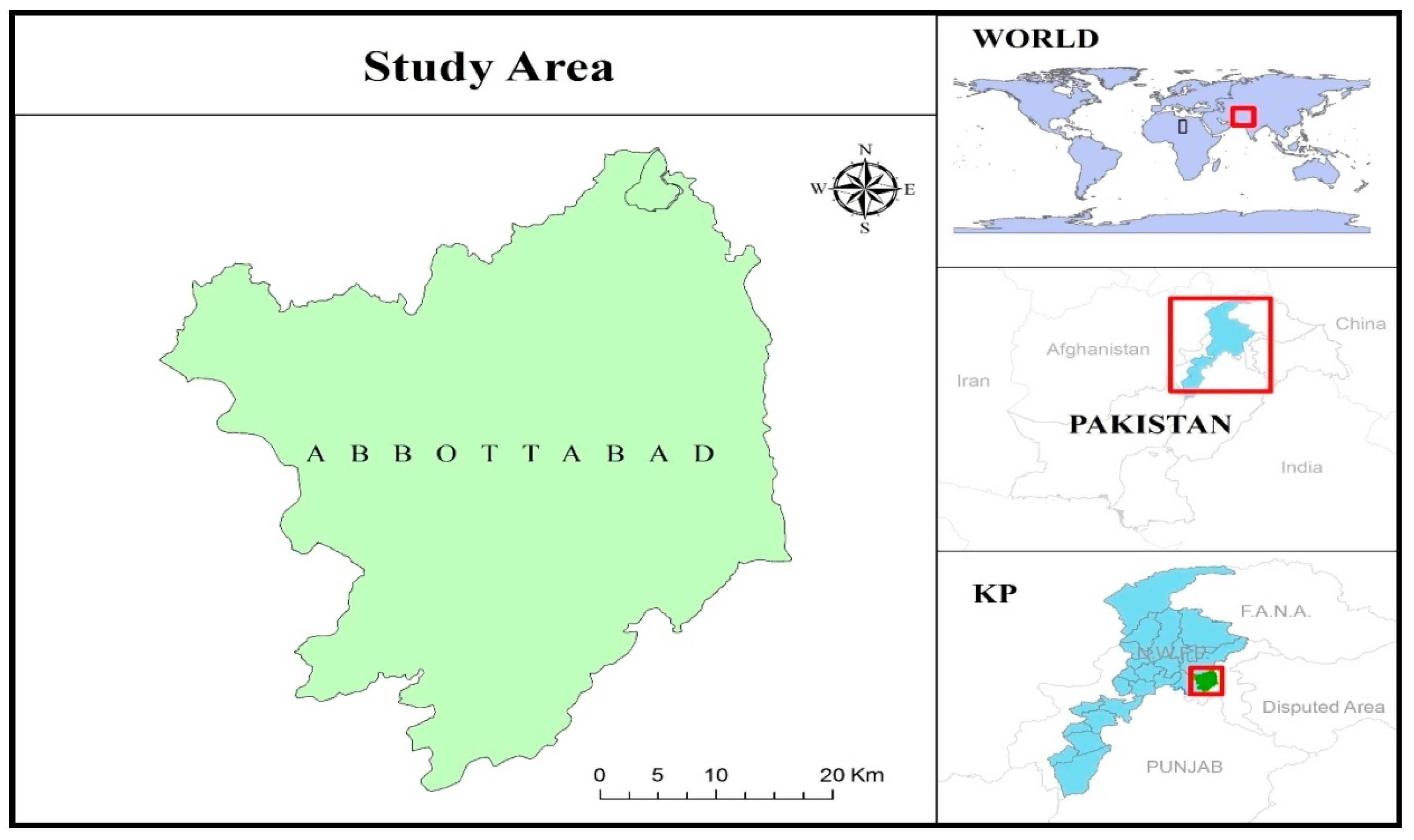
2.1. Study Area—Abbottabad
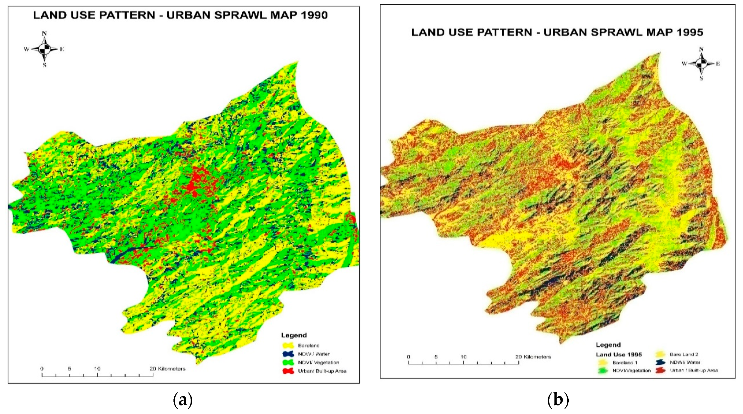
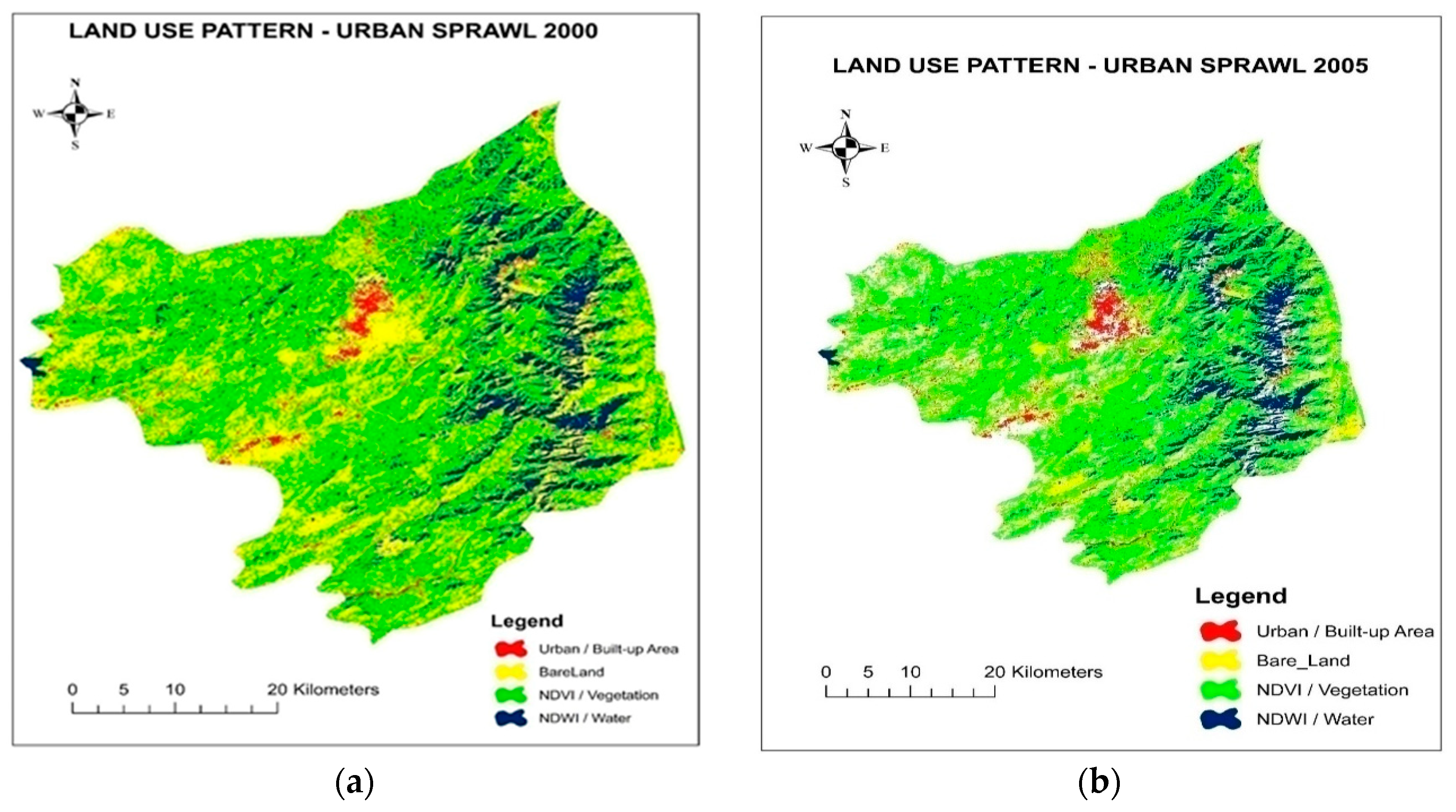
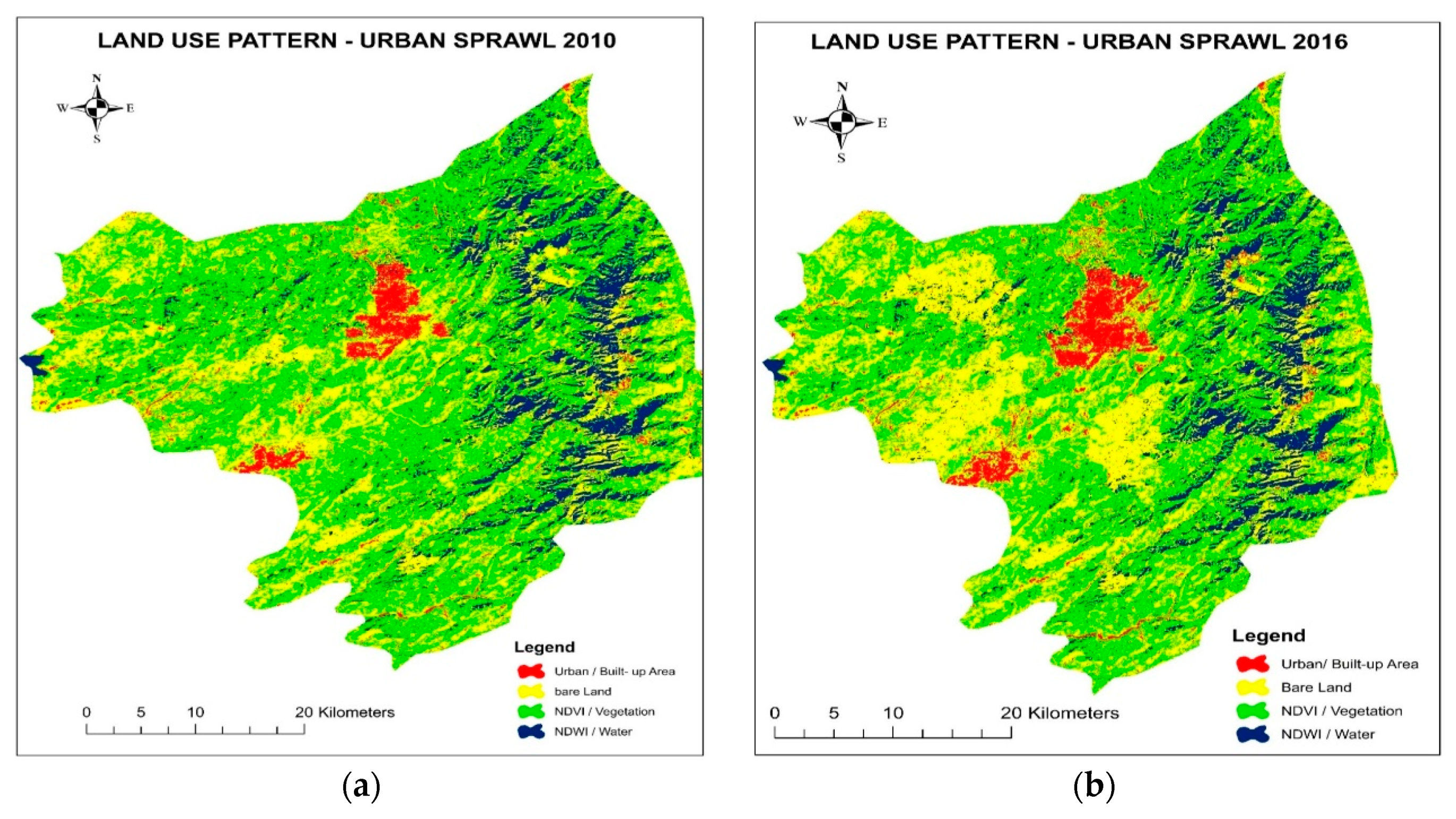
District Abbottabad was named after its founder first Deputy Commissioner Major James Abbot in 1853. This valley was the official headquarters of district of Hazara and later on became division [15]. Abbottabad is situated at an elevation of 1256 m above sea level in the north of Khyber Pakhtunkhwa (KP) province of Pakistan. Area wise, it is spread over 1967 square kilometers. It is surrounded by Mansehra District, Muzaffarabad District, Rawalpindi District, and Haripur District from north, east, south, and west respectively. It is located at a distance of 120 km from Rawalpindi, 217 km from Peshawar, and 84 km from Kohala Bridge. Map of study area is shown at Figure 1. Abbottabad is mostly a rugged mountainous region with mean maximum temperature of 23 °C and minimum temperature of 11 °C. Altitude of the region varies from 600 m to 2800 m and its climate varies accordingly. In winters, mostly snowfall is experienced above the height of 900 m which includes areas of Galyat, Barian, and sometimes in the city of Abbottabad. Monsoon rainfall occurs from the start of July till September and then a dry spell remains for two months afterwards. The River Kunhar, a famous stream, flows sideways from the north eastern boundary of the district and it links in the east with another major stream: The River Jhelum. A number of streams flow through district Abbottabad and most significant amongst them are Harro, Dor, and Siran. Besides the study area, two major parts of methodology are adopted i.e., Urban Sprawl (including NDWI, NDVI, and NDBI) and methods of LST extractions from multispectral images.

2.2. Urban Sprawl

Urban sprawl is extracted from the multispectral images by using following methodology.

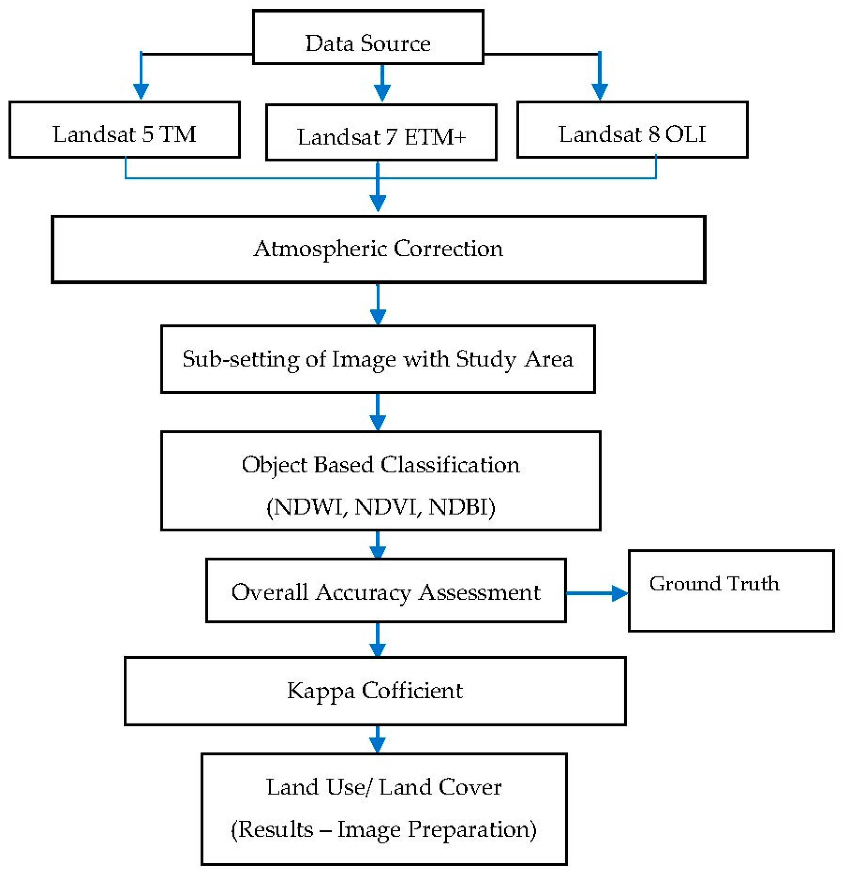
2.2.1. Data Collection and Pre-Processing

Satellite data was obtained by the website (www.earthexplorer.usgs.gov) owned by USGS. It provides data free of cost. TIR imagery of Landsat 5, Landsat 7 ETM+ and Landsat 8 (OLI) with path 150, row 36 was collected. Object-based classification was applied on the subset of study excluding TIR band using ERDAS Imagine including layer staking. ENVI-2014 Software was used for pre-processing. Band combination of 7-2-1, 4-3-2 and 1-4-5 were used to detect urban, vegetation and water zones in object-based classification in the study area from 1990–2016 with the interval of five years length. Resolutions of the images was 30 m. Complete details of the various images are depicted in Table 1, details of constant values for LST is given in Table 2 and processes of methodology till final output of maps are shown in a flow chart at Figure 2. However, numerical outputs of different indices are shown in Table 3.

2.2.2. NDWI (Normalized Difference Water Index)

Landsat imageries of different years i.e., 1990, 1995, 2000, 2005, 2010, and 2016 are taken in which urban increase is distinguished besides other common indices. The range of land and water mask (LWM) varied from 0–255. The range of water was observed from 0 to 57; however, the range of shallow water was observed from 28 to 37. The water classes were extracted utilizing Equations (1) and (2) [16]. These equations were perfectly suitable for separating water class from the image and mapped into six maps as shown into the Figure 3, Figure 4 and Figure 5.
NDWI   = Green NIR Green + NIR
LWM   = IR Green × 100

2.2.3. NDVI (Normalized Difference of Vegetation Index)

NDVI is calculated from Equation (3). In NIR Band (band 4), it has been witnessed that reflection of vegetation was much higher than that of visible bands. For the extraction of vegetation index, red band was deducted from NIR and then divided by sum of NIR and red bands in all Landsat images, which represent the ratio from −1 to +1 and mapped in Figure 3, Figure 4 and Figure 5 in the dense green vegetation [17]. It was observed that high reflectance remained persistent in NIR band. Usually, values of NDVI remain between −1 and +1 [18].
NDVI   = NIR Red NIR + Red

2.2.4. NDBI (Normalized Built-Up Index)

NDBI was derived from Equation (4). Built-up area was calculated by deducting vegetation and water indices from the images. In e-Cognition software, NDBI was calculated from Landsat TM sensors Band 5 value is subtracted from Band 4. For this whole process, object-based classification was used, where each and every object of the built-up area was considered to classify and exported in shapefiles with the calculation from following equations [19]. Built-up area is derived from Equation (5).
NDBI   = Band   5 Band   4 Band   5 + Band   4
BUA   =   NDBI NDVI

2.2.5. Object Based Image Classification

To extract different classes from the six images of different years, object-based images classification was used by incorporating eCognition software. This classification depends upon geometry, structure information and spectrum character [20]. There are two basic approaches or steps which are used to classify an image, i.e., segmentation and classification of segmented image through classifier [21], these are:
  • Segmentation
Multiresolution Segmentation algorithm was used for multiscale segmentation. To produce polygons, the images were disintegrated into many segmentations by determining their layer weight, shape, scale parameter and compactness [22]. In segmentation, layer weight was set as “1” for each layer, scale parameter was “25”, shape of each segment was “0.2” and compactness was “0.8”.
b.
Classifier
After setting up the semination parameters, classification method was adopted using KNN Classifier. Detail of hyperparameters of the classifier was N_neighbor: “default” (default parameter was used = 5), Weight was “uniform”, auto algorithm, Metric was “minkowski” (where values of “P” was 2), Metric_params were “none” and N_jobs: “none”. After that final classified images were established.

2.2.6. Overall Accuracy Assessment and Kappa Coefficient

Accuracy assessment was measured to assess quality of results of any classification which gives us evidence of reliability of classifier. Accuracy assessment was governed by validation based on “Ground Truthing” and “Referenced Points” [23] which are depicted in Table 4. Accuracy assessment and Kappa Coefficient were estimated with the help of ArcGIS software and statistics. Confusion metrices were established after object-based classification [24]. Overall an average of 160 points were earmarked on each classified image and the same points were validated on the ground by using GPS. Kappa coefficient was a discreet multivariate technique that was used for accuracy assessment [25]. These methods validate the results. Equations (6) and (7) were used for calculation of Kappa Coefficient (as mentioned below).
k ^ = N   Σ r = 1 r X i i     Σ r = l r   ( x i +   ×   x x + i ) N 2   Σ r = l r   ( x i +   ×   x x + i )
k ^ = ( T o t a l × S u m   c o r r e c t )   S u m ( r o w × c o l u m n ) Total   Squared   S u m   ( r o w × c o l u m n )

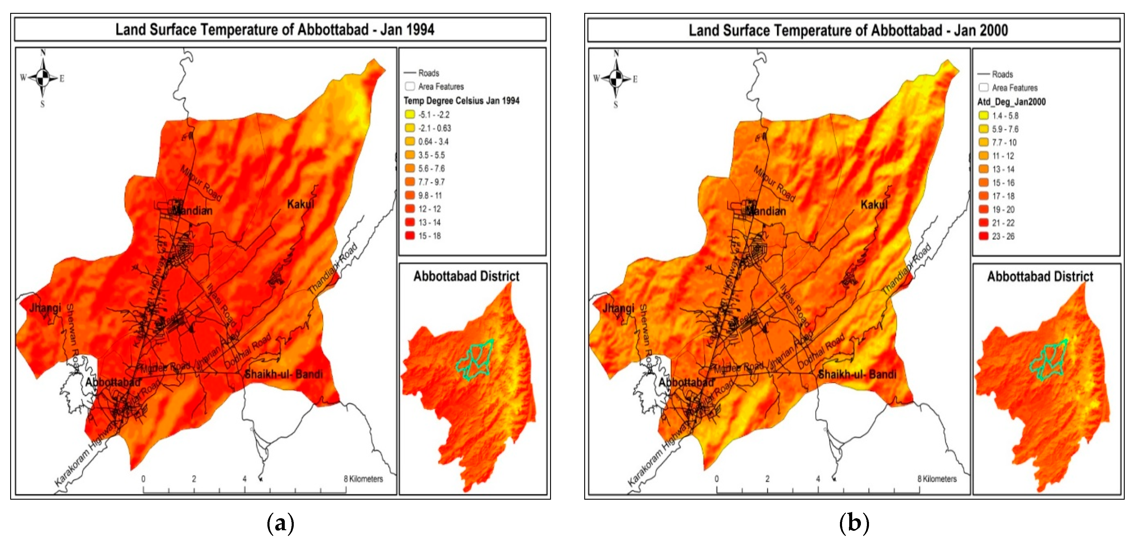
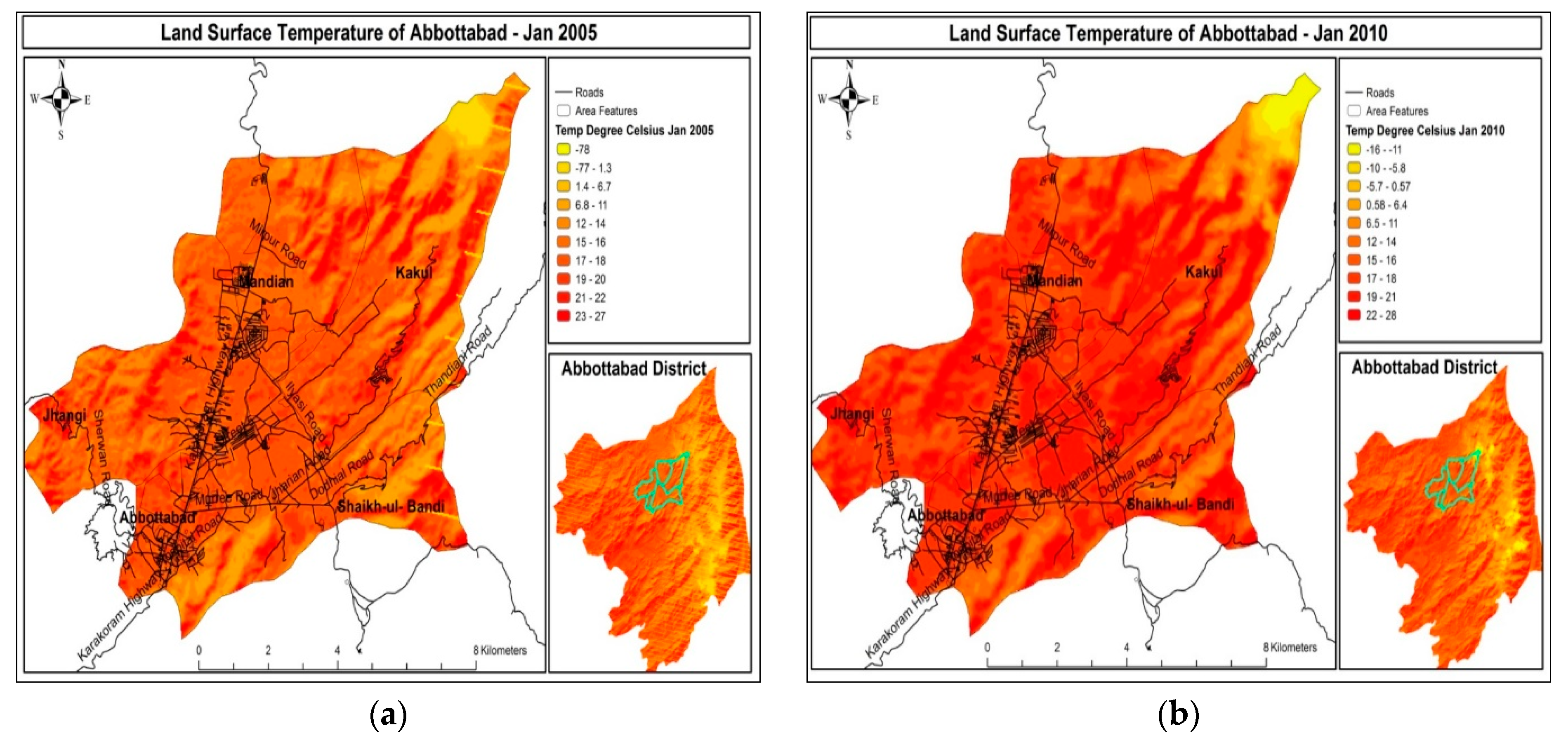
2.3. Extraction of Land Surface Temperature (LST)

2.3.1. Data Collection and Compilation

Data pertained to thermal infrared images (TIR) of Landsat 5 TM to Landsat 8 (OLI) was used in this study for LST. Data were procured from USGS resources from 1990 to 2016 with the interval of five years; the collection of data was carried out from 1994–2000 from Landsat 5 TM collection and from 2001 to 2013 from Landsat 7 ETM+ in the same pattern. The details of images for months of Jan 1994–Jan 2016 and Jun 1994–Jun 2016 are given in Table 2. Images of complete months of Jan and Jun were downloaded then all the images of each month were stacked into one image. Then images of complete five years were stacked and used for average of LST of five years.

2.3.2. Conversion of DN Values to Physical Units

The processing of images was carried out in floating points 32–bit. These images were processed in units from irradiance to absolute radiance. Finally, 32-bit image was converted in to integer form of 16-bit instead of floating form with the original level 1 format. With the help of metadata file (having different values of different bands), images had been converted from spectral radiance to radiance as famous as physical unit. This conversion is computed from the equation mentioned below:
  L λ =   M L × Q c a l +   A L
L λ = S p e c t r a l   r a d i a n c e   ( W / ( m 2 ×   s r   ×   μ m ) )
M L = R a d i a n c e   m u l t i p l i c a t i v e   s c a l i n g   f a c t o r   f o r   t h e   b a n d ( f r o m   t h e   m e t a d a t a )
Q c a l = L 1   p i x e l   v a l u e   i n   D N
A L = R a d i a n c e   a d d i t i v e   s c a l i n g   f a c t o r   f o r   t h e   b a n d   ( f r o m   t h e   m e t a d a t a )

2.3.3. Top of Atmosphere Reflectance

L1 images are normally changed into integer value of 16 bit to TOA reflectance. The equation mentioned below was used for the conversion.
  ρ λ =   M ρ × Q c a l +   A ρ
ρ λ = T O A   P l a n e t a r y   S p e c t r a l   R e f l e c t a n c e ,   w i t h o u t   c o r r e c t i o n   f o r   s o l a r   a n g l e .   ( U n i t l e s s )
M ρ = R e f l e c t a n c e   m u l t i p l i c a t i v e   s c a l i n g   f a c t o r   f o r   t h e   b a n d ( f r o m   t h e   m e t a d a t a ) .
Q c a l = L 1   p i x e l   v a l u e   i n   D N
A ρ = R e f l e c t a n c e   a d d i t i v e   s c a l i n g   f a c t o r   f o r   t h e   b a n d ( f r o m   t h e   m e t a d a t a ) .

2.3.4. DN to Brightness Conversion for Kelvin Temperature

Temperature in Kelvin degree was computed by conversion of Thermal Infrared satellite (TIRS) data. This temperature was computed using satellite prescribed emissivity from its metadata file. Equation (10) explains procedure of Kelvin temperature from the satellite images after conversion into brightness temperature. Constant value of emissivity was 0.95. Constants of below equation are mentioned in Table 2.
  T = K 2 ln ( K 1 L λ + 1 )
T = T O A   B r i g h t n e s s   T e m p e r a t u r e ,   i n   K e l v i n .
L λ = S p e c t r a l   r a d i a n c e   ( W a t t s / ( m 2   s r     μ m ) )
K 1 = T h e r m a l   c o n v e r s i o n   c o n s t a n t   f o r   t h e   b a n d   ( f r o m   t h e   m e t a d a t a )
K 2 = T h e r m a l   c o n v e r s i o n   c o n s t a n t   f o r   t h e   b a n d   ( f r o m   t h e   m e t a d a t a )

3. Results

Two types of results are discussed in successive paras, i.e., Urban Sprawl (including Land use and Land Cover) and results of LST.
Figure 3a,b are showing a major increase in built-up area. In 1990, urban area was 9.07%, vegetation 39.14%, water 26.64% and bare land were 25.13%. In 1995, urban area was increased from 9.07% to 10.15%. Vegetation decreased from 39.14% to 38.39%, water 26.64% to 25.94% and bare land was increased from 25.13% to 25.49%.
Figure 3. (a) Land use pattern of urban sprawl 1990; (b) land use pattern of urban sprawl 1995.
Land 10 00095 g003
Figure 4a displays results of 2000, built-up area/urban area was increased up to 11.27%. Vegetation increased from 38.39% to 39.61% (city government planned to plant more than 700,000 trees [26]), water decreased from 25.94% to 24.377% and bare land was also decreased from 25.49% to 24.733%. Figure 4b is portraying a glaring variation in land cover change. In 2005, built-up area/urban area was increased from 11.27% to 14.72%. Vegetation decreased from 39.61% to 33.04%, water decreased from 24.377% to 22.75% and bare land was also increased from 24.733% to 29.469%.
Figure 4. (a) Land use pattern—urban sprawl 2000 and (b) land use pattern—urban sprawl 2005.
Land 10 00095 g004
Figure 5a is projecting an enormous change from the Figure 4a,b. Where built-up area increased from 14.72% to 16.5%. It happened because of IDPs and people migrated from Balakot, Rawalakot and erstwhile federally administrated agencies to Abbottabad city and its fringe areas as it is a safe place and well settled in terms of all basic amenities of life [27]. However, Figure 5b is illustrating a gigantically great difference in land cover change from all the figures from Figure 3 to Figure 5. In Figure 5b, urban sprawl increased from 16.5% to 24.22%. This increase is more than 275 times from 1990 that shows that rapid urban growth in the study area. This increase brought about many other changes in micro climate as well as land cover. A glaring change resulted due to built-up that followed by vegetation decreased from 30.59% to 25.39%, water decreased from 17.81% to 12.69% and bare land was also increased from 35.03% to 37.68% that will be the part of urban dwelling in future. This change is due to a settled influx in the study area which brings about the cause of continuous microlevel change in the environment. Its proof is a decrease of vegetation and water sources as well as water reservoirs that is shown in Table 3 and its graphical representation is shown at Figure 6.
Figure 5. (a) Land use pattern—urban sprawl 2010 and (b) land use pattern—urban sprawl 2016.
Land 10 00095 g005

3.1. Results of Overall Accuracy and Kappa Coefficient

Results of the accuracy are shown as per values of Table 4 (classification fields) the classes which have been calculated and checked are water, vegetation, urban or built-up and bare land. Producer’s accuracy and User’s accuracy are mentioned in the Table 4 a,f, however, overall accuracy of six classified maps is 91.2%, 81.25%, 90.86%, 93.75%, 92.5%, and 90.63%. Kappa Coefficient used which is one of the most common means of expressing classification accuracy [28]. The table shown here is known as error matrix, it compares on a category by category basis, the relationship between known referenced data (Ground Truthing) and the derived results. When Khat is ranging the values with >0.80; it is considered as strong accuracy, from 0.40 to 0.80 very good accuracy and when coefficient is <0.40 then it is believed poor accuracy [29]. Thus, accuracy of the images was proved as strong accuracy.

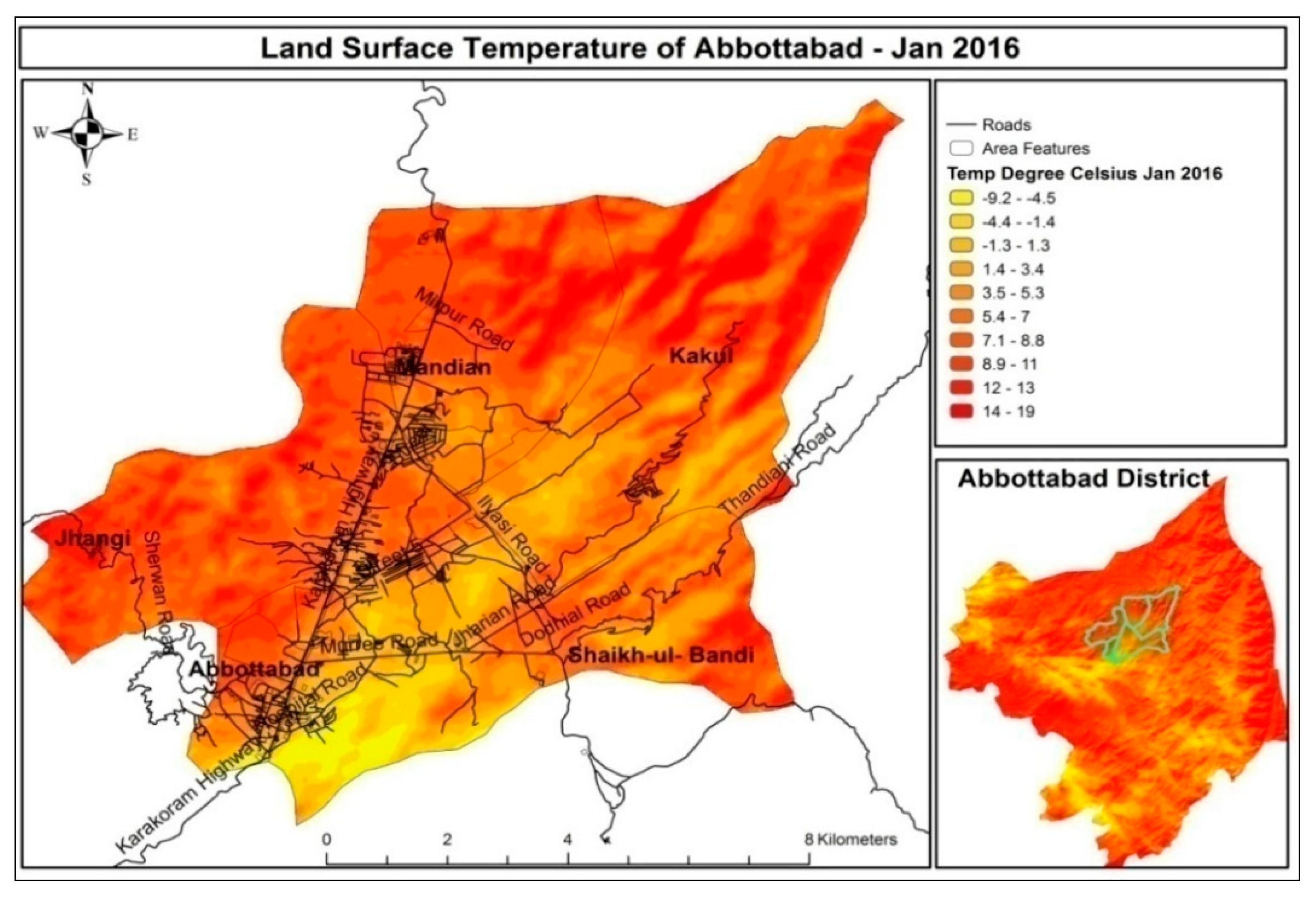
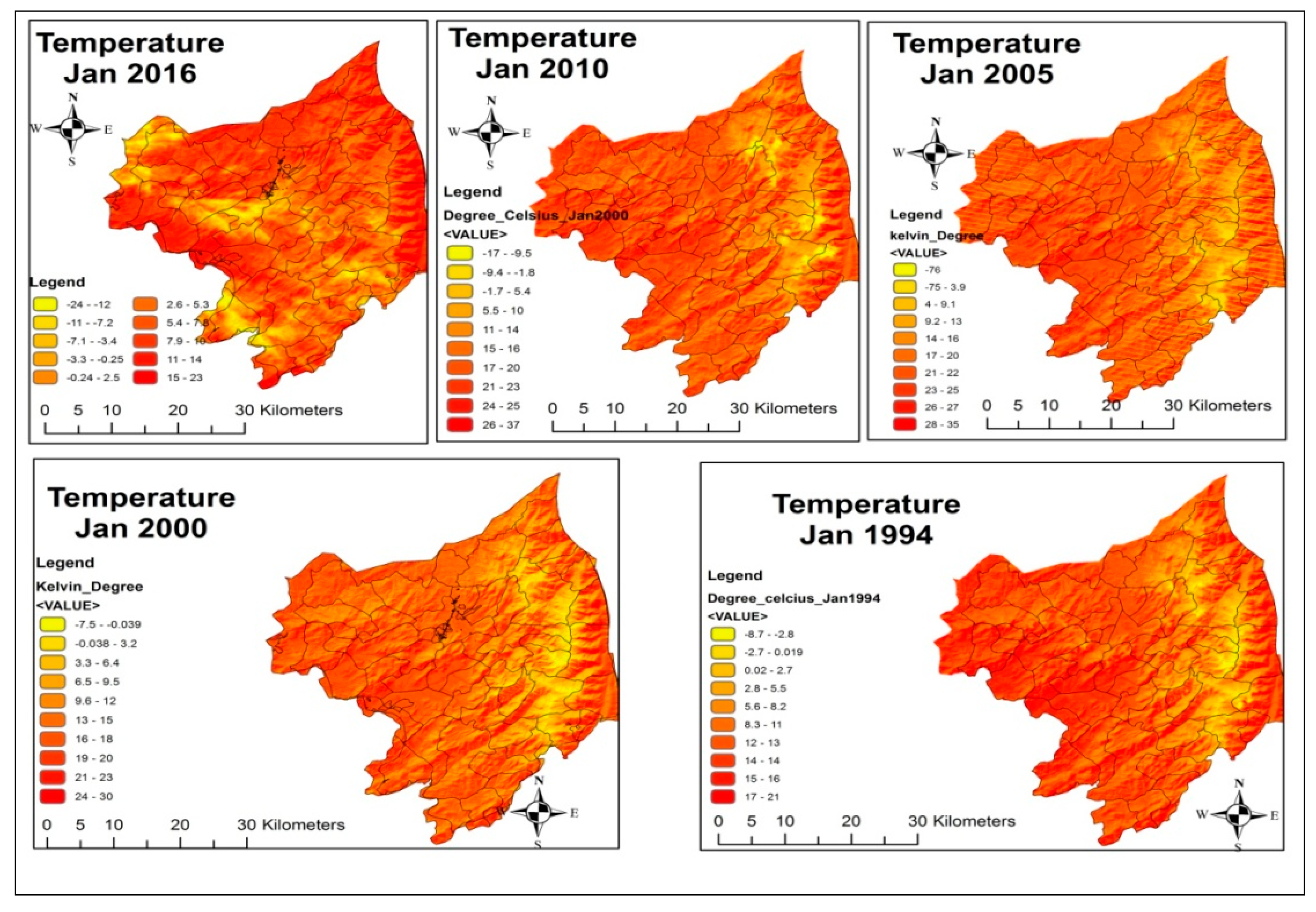
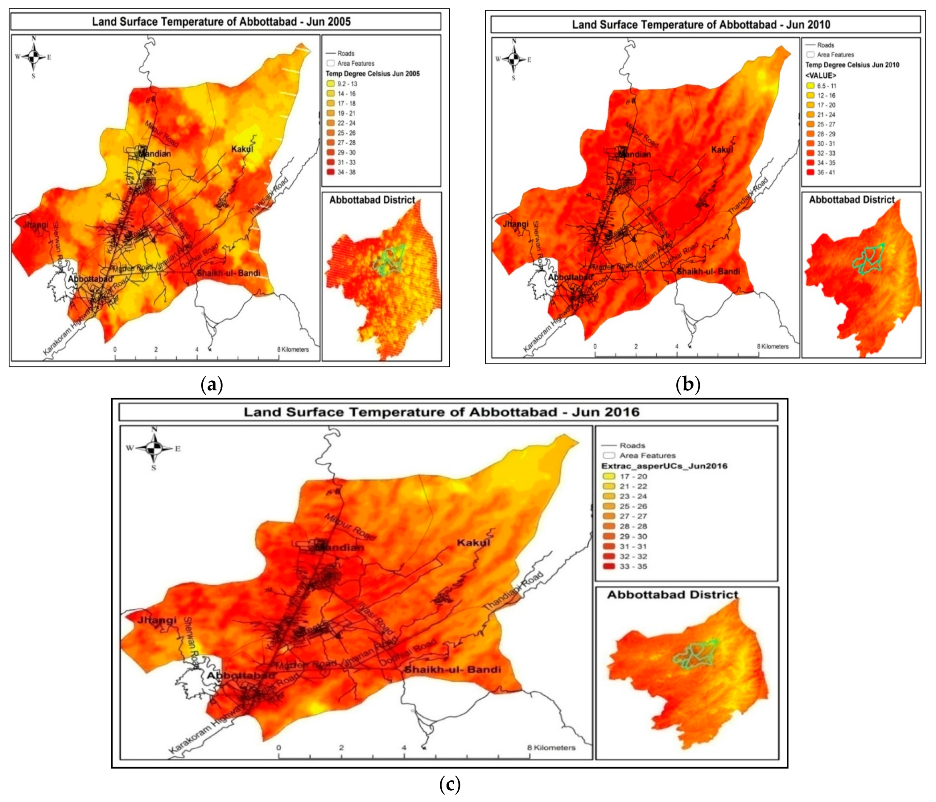
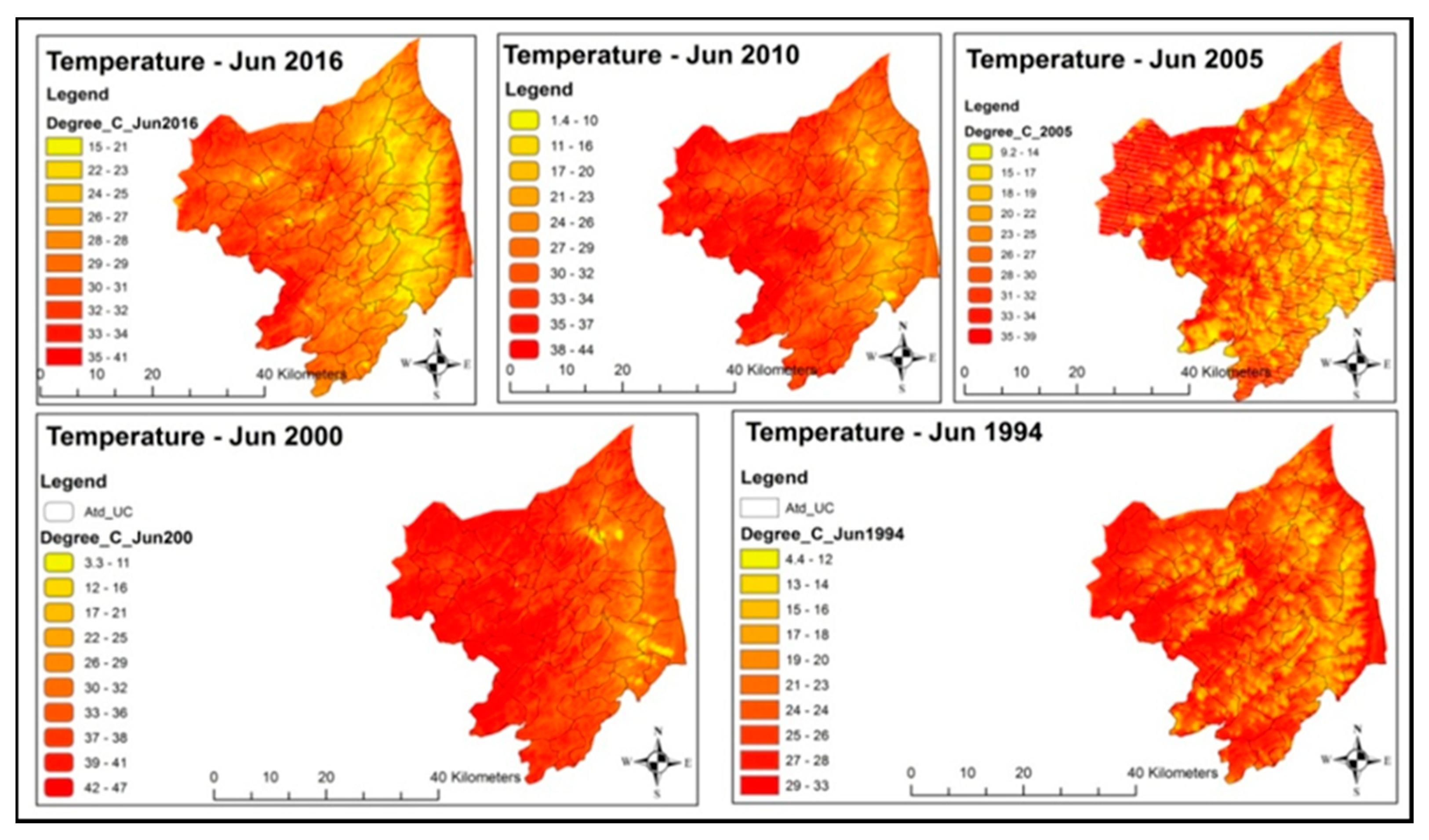
3.2. Results of Land Surface Temperature (LST)

LST means surface temperature on the ground or surface of the earth. This surface temperature is not easily measured and observed with naked eyes [30]. However, this surface temperature is very much measurable through various new technologies of satellites have thermal recording sensors [31]. Figure 7a showing temperature of 1990–1994 and Figure 7b depicts temperature of 1995–2000 for the months of Jan. City center is showing high temperature because of concrete surfaces. Minimum LST of Abbottabad from Jan 1995–2000 is shown that it was increased from 3 °C to 5.8 °C. In Figure 7a the temperature of Abbottabad has risen up to 20 °C. A glaring change is very much pertinent to perceptible interpretation held in the figure. In the map all three Union Councils have different temperature values from 25 °C to 26 °C.
In view of Figure 8a, temperature was increased gradually from 2000 to 2005. There has been an increase of almost 1 °C in the six years from 2000 to 2005. The overall temperature extent of Abbottabad varied from 12 °C to 27 °C. The extent of temperature has again increased from 6.5 °C to 28 °C in 2010. Accumulatively, 1 °C temperature has again increased within five years of time span from 2006–2010 as shown in Figure 8b.
From Jan 2011–2016, a drastic change in temperature was witnessed because heavy snowfall was experienced in 2016 after almost 30 years as shown in Figure 9. This snowfall phenomenon is also directing us towards the existence of extreme climate changes from micro to macro level. At minimal level temperature decreased up to −4 °C to −5 °C. At maximum level the same decrease was witnessed more than 10 °C temperature within six years’ time span. Complete belt of urban land cover including Abbottabad city, Mandian, Nawansher, Jhugiyan, Shimla hill, and Abbottabad villages experienced extreme cold temperature ranging up to −9.2 °C, after a heated spell which was being experienced since last 15 years. Figure 10 is showing all the LST maps in a single glance which is depicting drift of increase and decrease temperature for the month of Jan 1990 to Jan 2016. Small set of boundaries in the maps are showing Union Council boundaries of District Abbottabad. The change in temperature at micro level within the Union Council boundaries of District Abbottabad has been increased accumulatively from 1 °C to 7 °C and the same decreased in the month of Jan2016 up to 10 °C in upper limit and −4 °C to −5 °C in lower limit. It is quite eminent that temperature of city of 25 years has a rising trend having a direct impact on air temperature as well.
From Jun 1990–1994, the temperature of Abbottabad city and its surrounding areas varied from 9.2 °C to 31 °C. Quality of satellite imagery taken for Jun 1990–1994 were comparatively good but cloud cover was 10%. However, cloud cover was removed by ENVY software using atmospheric correction, even then complete clouds could not be eliminated completely, because of cloud thickness and their location near to the surface. Change in temperature was observed in Figure 11b from 14 °C to 38 °C in Abbottabad city and surroundings. In Figure 11a,b, the temperature of Abbottabad has risen up to 9 °C. Average temperature of these months from 1990 to 2013 remained at 32.3 °C. While maximum temperature of the city center rose up to 41 °C which is abnormal for a hill station city like Abbottabad. Figure 12a–c indicate that average temperature of Jun from 2001 to 2016 remained 33.4 °C which shows 2 °C increased within last five years’ time period. Temperature change within the city and surrounding areas observed from rise of 1 °C to 4 °C. Minimum temperature has been derived from the satellite images is 19 °C and maximum is 38 °C.
Figure 13 shows all the LST maps which is depicting increase and decrease temperature for the month of Jun 1990 to Jun 2016. Temperature has been increased accumulatively from 1 °C to 8 °C in the city as well as the district and the same increased in the month of Jun 2011–2016 up to 8 °C in upper limits of the district and 12 °C in lower limit of the district. As per derived LST of Abbottabad city is within the bounds of 20 °C to 27 °C whereas average temperature of these months remained 33 °C as per the record of PMD (Pakistan Metrological Department) Kakul station as shown in the graphs (Figure 14 and Figure 15).

4. Discussion

Urban Sprawl is expanding rapidly not only in Pakistan but also in other countries of South Asia as well as Asian continent as a whole. Framework of Economic Growth (FEG) of Planning Commission of Pakistan 2011 has emphasized on the need of change of planning department for solving urban sprawl issues, to convert “lethargic” cities to innovative urban societies and hub of new commercial innovations [32]. Deterioration of urban planning is not new in Pakistan [33]. It is also available in many cities of other countries of South Asia as well other world [34]. This study indicates that urban sprawl adversely affects the microclimate, and as a result the poor community may be more vulnerable to this change. Thus, increasing of temperature may give rise to glaciers melting and glaciers related hazards may increase near such cities located in the northern areas of Pakistan. As a result, decreasing agricultural and receding livestock production, degradation of ecosystem, and biodiversity loss may hamper the urban environment.
Microclimate is determined by many factors as when sun rays strike the surface of the earth, it expands in the noon or day time and contracts in evening or at night. At noon the temperature touches its peaks and at mid night temperature decrease at minimum level. This diurnal change of temperature can only alter the weather at short span of time whereas its permanent change throughout the year and continue this time span change the climate permanently. In this scenario, Griffith Tylor’s environmental determinism school of thought confirms such change of phenomenon [35]. If it happens continuously from gradual to maximized intensity in terms of time and space, it refers to global warming. Global warming occurs due to various causes and happenings including rise of pollutants in the air in the form of industrial waste, CFC gases, carbon addition from coal burning, emission of carbon-monoxide from vehicles, dust from biological weathering, and numerous other pollutant materials in the air; which absorb the heat and trap the sun radiation resultantly this heat blankets the Earth’s surface that bring about the rise in surface temperature. Dataset of Abbottabad station was in mean monthly, which was converted into mean annual, and obtained only one value from twelve months of data, and then plotted. Resultantly outputs we get are explained in the succeeding paragraphs and figures. In the graphs from Figure 14 and Figure 15, it is clearly evident that temperature in 1953 was above 24 °C, decreased up to 22 °C till 1957, then abrupt change is witnessed in the graph. Temperature fluctuation is less varied between 1953 to 1970 which is from 22.6 °C to 24.4 °C less one year which is 22 °C in 1957. After 1970, temperature decreased from 24.4 °C to 22 °C and remained stable in between 21.5 °C to 23.5 °C from 1971 to 1998 but after this temperature abruptly and drastically increased till 2000 onwards because of change in land cover, i.e., urban sprawl increased resultantly microclimate is changed in the context of standard deviation, the below figure shows that temperature deviated from 5.6 °C to 8.1 °C. This change is the major change in the whole mean temperature.
In Figure 16, a comparison of land surface temperature calculated and air temperature collected from Kakul weather station for the month of Jun is made from the year 1990 to 2016. It can be seen that as LST is increasing, so does the air temperature. LST has risen from 31 °C in 1990 to 38 °C in 2016. In the same manner the air temperature also rose to 2 °C in 26 years which is startling, even as per the international standards. We can also observe that LST is comparatively higher than that of air temperature, reason being ground and especially hard constructed surface retain more heat than that of atmosphere. Urban sprawl rise in the past 16 years without any planning has become the main reason for this alarming rise. In Figure 17, a comparison of land surface temperature calculated and air temperature collected from Kakul weather station for the month of Jan is made from the year 1990 to 2016. LST has risen from 18 °C in 1990 to 21 °C in 2016. In the same manner the air temperature also rose by 1.7 °C in 26 years. We can also observe that LST is comparatively higher than that of air temperature, reason being ground and especially hard constructed surfaces like roads and buildings retain more heat than that of atmosphere. Urban sprawl in the past 16 years without any planning has become the main reason for this alarming rise. Figure 18 gives clear comparison that microclimate change of temperature due to urban sprawl.
Besides Abbottabad, it is very evident in many cities of South and South East Asian countries like Hong Kong SAR, Shenzhen, Seoul, and Singapore have been devasted in urban planning as well as urban green environment due to rapid their growth and economic infrastructures [36].
This research will enlighten the researchers how urban sprawl is happening in one of the emerging cities of Pakistan. It advances our understanding regarding diurnal to yearly variations in temperature in a mountainous urban area that is located in the way of famous China–Pakistan economic corridor (CPEC). The study highlights the changing of surface temperature in an elevated terrain and reports how temperature between urban and non-urban lands affects not only microclimate but also energy transfer and overall habitability of urban areas [37]. Such unsustainable developments effect the natural process of energy transfer and heat up the urban materials to affect general environmental and micro climatic patterns. So, in this case, this study suggests the developments on environmental and social concerns.
Today, we are expanding cities without focusing on deadly consequences for nature and its cycles such as water distribution or availability, vegetation effects on its neighborhoods, ecosystems depletion, and gradual disruption of temperature balance. These planning practices can be witnessed in major south Asian countries like India and Pakistan, resulting in drastic influences on mean temperature distributions [38]. The decrease of vegetation areas has further aggravated the situation; often planners neglect smaller green spaces like linear strips along the roads or tree clusters planted nearby parks or recreational lands. Such micro level urban developments can provide local cooling benefits that affect the microclimate of the surrounding localities through vegetation and evapotranspiration processes. These vegetation and water scarcity have worse implications for modern planners to design the next master plans including vegetation areas and strips in down and uphill parts of such cities. These enhancements tend to produce effective cooling effects that can diminish adverse impacts of urban heat island (UHI) [39].
Studies like this research have been done previously which highlight the relationship between urban sprawl and water depletion in such a water potential area [40]. The planners can investigate such changes and find the major causes behind these variations. This study will also provide a practical guide to initiate advanced researches to relate urban sprawl with microclimate as well as environmental developments in the world.
The combination or integration of contemporary geographic information (GI) and remote sensing (RS) tools with urban planning in microclimatic assessment perspectives is a complex task but has promising tomorrow. These sorts of integrations offer climatic evaluation as a fragment of overall urban planning and no additional endeavors are needed that prove their cost-effectiveness and time effectiveness because planners can also assess the salient influences of urban processes down to microclimatic levels thus revealing overall urban morphology [41]. Such findings answer policy questions such as: Where temperature is higher and how can it be lessened via planting trees in clusters or strips? What impacts these changes caused uphill, especially in water-associated scarcity context? How can we improve such microclimatic adversities? Further to more advanced levels, a real-time environmental monitoring and assessment platform may be established through internet of things (IoT), locational transformation (LT), and GI intelligence technologies (GIIT), to address real-time socio-environmental and microclimatic problems. This level belongs to fourth industrial revolution (industry 4.0) which is far from developing countries of South Asia and especially Pakistan; we still tremendously lack geographic enlightenment at organizational level and major geographical corridor is yet to be established where smart urban planning may be integrated with such modern big datasets. This study leads us towards such paths after revealing major urban induced problem effecting physical and social environments. The use of such platforms (with IoT, LT, and GIIT) can unleash great urban planning possibilities with public and organizational participation for sustainable development [42]. Another perspective for our cities can be advised in two directions as suggested by many researchers that we have to change our manufacturing and consumption habits to achieve effective sustainable growth. Due to these habits, we are building more unsustainable land uses and causing deforestation in many areas of the world (especially developing countries) [43]. Natural environments are shrinking due to increasing residential as well as commercial demands. Thus, urban systems are complex and always evolving to create new opportunities and problems, so we need to transform our society according to modern dynamics by educating our citizens and planners to establish new effective ways of development.
In this study we have utilized Landsat data due to its free availability. Further to this, international researchers may adopt following to learn more techniques for establishing urban sprawl and LST relationships:
  • Usage of high-resolution remote sensing data which may give more accurately analysis.
  • Access hydropower protentional in the region which can be access using in-suit data of perennial streams which is abundantly available. However, in future research, we will use ground water storage (GWS) monitoring system such as GRACE (Gravity Recovery and Climate Experiment) mission to access the ground water variation to access the impact of climate variability on GWS.
  • Access data through machine learning techniques by developing application programming interfaces (APIs).

5. Conclusions

Due to enormous microclimate change in Abbottabad, there was a dire need to know about the reason of this microclimate change. It was revealed that it was happening due to drastic increase of urban sprawl, and importance of this research was magnified. On the basis of our results, our research hypothesis was supported. Moreover, this research will be an eye-opener for the city management authorities to monitor urban sprawl and mitigate microclimate change.
Microclimatic change has been witnessed due urban sprawl, deforestation, housing colonies and rural/urban settlements. Urban sprawl is increased 178 to 477 sq. km within the years 1990 to 2016. Vegetated area has decreased from 770 to 602 sq. km. Surface and inland water confined areas had also decreased from 524 to 360 sq. km within the last 26 years. The bare land has increased from 494 sq. km to 742 sq. km which is under urban settlements near the city. Increase in temperature as well as climatic drift at micro level in the urban built-up area of Abbottabad has been observed and extreme climatic temperatures are being experienced due to unplanned urban sprawl. LST in winters has risen from 17 °C to 23 °C and at times shoots up to 31 °C which is alarming. Air temperature has also increased from the 1980s to 2016 at a steady rate with the annual mean temperature rising by 3 °C to 4 °C. During summers average air temperature rose up to 33 °C from 28 °C and LST has a steadily risen from 28.4 °C to 35 °C. Time series analysis showed that overall increase of temperature was gradual even witnessed at micro level.

Author Contributions

Conceptualization: L.A.W., M.A.H.K. and S.A.A.N. Methodology: M.A.H.K., H.B.H.A. and Z.H.J. Software: M.A.H.K. and L.A.W. Validation: S.A.A.N., D.H. and Z.H.J. Formal Analysis: L.A.W., M.A.H.K., D.H. and Z.H.J. Investigation, L.A.W., M.A.H.K. and S.A.A.N. Data Curation: M.A.H.K. and H.B.H.A. Writing—Original Draft Preparation: M.A.H.K. D.H. and H.B.H.A. Writing—Review and Editing: L.A.W., S.A.A.N. and Z.H.J. Visualization: M.A.H.K., D.H. and L.A.W. Supervision: M.A.H.K., L.A.W., S.A.A.N. and Z.H.J. Project Administration: M.A.H.K. and H.B.H.A. Funding Acquisition: L.A.W., S.A.A.N., D.H. and Z.H.J. All authors have read and agreed to the published version of the manuscript.

Funding

This research received no external funding.

Data Availability Statement

Data used in this study will be available upon request from the first author.

Acknowledgments

We acknowledge emphatically towards services of Amir Iqbal (IST Islamabad), USGS for extending facilities of data downloading, Pakistan Metrological Department (PMD) and Kakul Met Station for the provision of weather data.

Conflicts of Interest

The authors declare no conflict of interest and the funders have no role in the design of the study; in the collection, analyses, or interpretation of data; in the writing of the manuscript, or in the decision to publish the results.

References

  1. Ministry of Climate Change. Framework for Implementation of Climate Change Policy; Ministry of Climate Change: Islamabad, Pakistan, 2014.
  2. Emadodin, I.; Taravat, A.; Rajaei, M. Effects of urban sprawl on local climate: A case study, north central Iran. Urban. Clim. 2016, 17, 230–247. [Google Scholar] [CrossRef]
  3. Yu, C.N. Spatial and temporal dynamics of urban sprawl along two urban–rural transects: A case study of Guangzhou, China. Landsc. Urban. Plan. 2007, 79, 96–109. [Google Scholar] [CrossRef]
  4. Shao, Z.; Sumari, N.S.; Portnov, A.; Ujoh, F.; Musakwa, W.; Mandela, P.J. Urban sprawl and its impact on sustainable urban development: A combination of remote sensing and social media data. Geo-Spat. Inf. Sci. 2020, 1–15. [Google Scholar] [CrossRef]
  5. Ghanghermeh, A.; Roshan, G.; Orosa, J.A.; Calvo-Rolle, J.L.; Costa, Á.M. New Climatic Indicators for Improving Urban Sprawl: A Case Study of Tehran City. Entropy 2013, 15, 999–1013. [Google Scholar] [CrossRef] [Green Version]
  6. Barrington-Leigh, C.P.; Millard-Ball, A. Global trends toward urban street-network sprawl. Proc. Natl. Acad. Sci. USA 2020, 117, 1941–1950. [Google Scholar] [CrossRef] [PubMed] [Green Version]
  7. Satterthwaite, D.; Huq, S.; Pelling, M.; Reid, H.; Lankao, P.R. Adapting to Climate Change in Urban Areas; International Institute for Environmental and Development: London, UK, 2007; Volume 58, ISBN 9781843696698. [Google Scholar]
  8. Tahir, A.A.; Muhammad, A.; Mahmood, Q.; Ahmad, S.S.; Ullah, Z. Impact of rapid urbanization on microclimate of urban areas of Pakistan. Air Qual. Atmos. Health 2014, 8, 299–306. [Google Scholar] [CrossRef]
  9. Mislan, K.; Helmuth, B. Microclimate. In Encyclopedia of Ecology; Elsevier BV: Amsterdam, The Netherlands, 2008; pp. 472–475. [Google Scholar]
  10. Nelson, K.C.; Palmer, M.A.; Pizzuto, J.E.; Moglen, G.E.; Angermeier, P.L.; Hilderbrand, R.H.; Dettinger, M.; Hayhoe, K. Forecasting the combined effects of urbanization and climate change on stream ecosystems: From impacts to management options. J. Appl. Ecol. 2009, 46, 154–163. [Google Scholar] [CrossRef] [Green Version]
  11. Kugelman, M. Urbanisation in Pakistan: Causes and consequences; NOREF: Oslo, Norway, 2016. [Google Scholar]
  12. Canada: Immigration and Refugee Board of Canada. Pakistan: Impact of the 8 October 2005 Earthquake on Activities of Police, Judiciary, Hospitals, Schools, Communication Systems, Transportation Systems; Institutions Issuing Identification Documentation; the General Situation in Affected Areas. Available online: https://www.refworld.org/docid/45f1480228.html (accessed on 8 October 2005).
  13. Hua, L.J.; Ma, Z.G.; Guo, W.D. The impact of urbanization on air temperature across China. Theor. Appl. Climatol. 2007, 93, 179–194. [Google Scholar] [CrossRef]
  14. Shashua-Bar, L. Microclimate modelling of street tree species effects within the varied urban morphology in the Mediterranean city of Tel Aviv, Israel. Int. J Climatol. 2010, 30, 44–57. [Google Scholar] [CrossRef]
  15. Review, A. Reconstruction, Earthquake Authority, Rehabilitation Authority Govt of Pakistan; UNESCO Office Islamabad: Islamabad, Pakistan, 2009. [Google Scholar]
  16. Fichera, C.R.; Modica, G.; Pollino, M. Land Cover classification and change-detection analysis using multi-temporal remote sensed imagery and landscape metrics. Eur. J. Remote Sens. 2012, 45, 1–18. [Google Scholar] [CrossRef]
  17. Wang, M. Understanding the Normalized Difference Vegetation Index (NDVI); Springer: Berlin/Heidelberg, Germany, 1987. [Google Scholar]
  18. Yengoh, G.T.; Dent, D.; Olsson, L.; Tengberg, A.; Iii, C.J.T.; Tengberg, A. Use of the Normalized Difference Vegetation Index (NDVI) to Assess Land Degradation at Multiple Scales; Springer: Berlin/Heidelberg, Germany, 2016. [Google Scholar] [CrossRef]
  19. Huiping, V.Y. Regional Urban Area Extraction Using MODIS data and DMSP/OLS data. In 2013 the International Conference on Remote Sensing, Environment and Transportation Engineering (RSETE 2013); Atlantis Press: Amsterdam, The Netherlands, 2013; Volume 1, pp. 292–295. [Google Scholar]
  20. Blaschke, T. Object based image analysis for remote sensing. ISPRS J. Photogramm. Remote Sens. 2010, 65, 2–16. [Google Scholar] [CrossRef] [Green Version]
  21. Aggarwal, N.; Srivastava, M.; Dutta, M. Comparative Analysis of Pixel-Based and Object-Based Classification of High Resolution Remote Sensing Images—A Review. Int. J. Eng. Trends Technol. 2016, 38, 5–11. [Google Scholar] [CrossRef]
  22. Wei, W.; Chen, X.; Ma, A. Object-oriented information extraction and application in high-resolution remote sensing image. In Proceedings of the 2005 IEEE International Geoscience and Remote Sensing Symposium (IGARSS ’05), Seoul, South Korea, 29–29 July 2005; Volume 6, pp. 3803–3806. [Google Scholar] [CrossRef]
  23. Verbyla, D.L. Practical GIS Analysis; CRC Press: New York, NY, USA, 2002; ISBN 9780203217931. [Google Scholar]
  24. Zhao, F.; Wu, X.; Wang, S. Object-oriented Vegetation Classification Method based on UAV and Satellite Image Fusion. Proc. Comput. Sci. 2020, 174, 609–615. [Google Scholar] [CrossRef]
  25. Congalton, R.G.; Mead, R.A. A quantitative method to test for consistency and correctness in photointerpretation. Photogramm. Eng. Remote Sens. 1983, 49, 69–74. [Google Scholar]
  26. KP-SISUG Pakistan: Provincial Strategy for Inclusive and Sustainable Urban Growth in Khyber Pakhtunkhwa Abbottabad City Developmemt Plan; Asian Development Bank: Mandaluyong, Philippines, 2019.
  27. Rashid, S.A. Mass Migration Affecting Abbottabad’s Demographic Balance. Int. News 2015, 16, 114. [Google Scholar]
  28. Gonzlez, R.C.; Bitterman, M.E. Resistance to extinction in the rat as a function of percentage and distribution of reinforcement. J. Comp. Physiol. Psychol. 1964, 58, 258–263. [Google Scholar] [CrossRef] [PubMed]
  29. Stehman, S.V. Estimating the Kappa Coefficient and its Variance under Stratified Random Sampling. Photogramm. Eng. Remote Sens. 1996, 62, 401–407. [Google Scholar]
  30. Walawender, J.P.; Hajto, M.J.; Iwaniuk, P. A new ArcGIS toolset for automated mapping of land surface temperature with the use of LANDSAT satellite data. In Proceedings of the 2012 IEEE International Geoscience and Remote Sensing Symposium, Munich, Germany, 22–27 July 2012; pp. 4371–4374. [Google Scholar]
  31. Carlson, T.N. Potential application of satellite temperature measurement in the analysis of land use over urban areas. Bull. Am. Meteorol. Soc. 1977, 58, 1301–1303. [Google Scholar]
  32. Planning Commission of Pakistan. Pakistan: Framework for Economic Growth; Planning Commission of Pakistan: Islamabad, Pakistan, 2011.
  33. Ministry of Climate Change. Challenges and Outlook of Pakistan Chapter 9. In Cycle; Ministry of Climate Change: Islamabad, Pakistan, 2011; Volume 1897, pp. 209–233. ISBN 9784431538592. [Google Scholar]
  34. Abaas, Z.R. Impact of development on Baghdad’s urban microclimate and human thermal comfort. Alex. Eng. J. 2020, 59, 275–290. [Google Scholar] [CrossRef]
  35. Meyer, W.B.; Guss, D.M.T. Neo-Environmental Determinism: Geographical Critiques; Palgrave Macmillan: London, UK, 2017; ISBN 9783319542324. [Google Scholar]
  36. Yuen, B.; Choi, S. Making Spatial Change in Pakistan Cities Growth Enhancing; World Bank: Washington, DC, USA, 2012. [Google Scholar]
  37. Kaloustian, N.D.Y. Effects of urbanization on the urban heat island in Beirut. Urban Clim. 2015, 14, 54–65. [Google Scholar] [CrossRef]
  38. Bandyopadhyay, S.; Pathak, C.R. Urbanization and Regional Sustainability in South Asia; Springer International Publishing: Berlin/Heidelberg, Germany, 2020; p. 332. [Google Scholar]
  39. Buyadi, S.N.A.; Mohd, W.M.N.W.; Misni, A. Vegetation’s Role on Modifying Microclimate of Urban Resident. Proc. Soc. Behav. Sci. 2015, 202, 400–407. [Google Scholar] [CrossRef] [Green Version]
  40. Song, J.; Wang, Z.-H.; Myint, S.W.; Wang, C. The hysteresis effect on surface-air temperature relationship and its implications to urban planning: An examination in Phoenix, Arizona, USA. Landsc. Urban. Plan. 2017, 167, 198–211. [Google Scholar] [CrossRef]
  41. Wong, N.H.; Jusuf, S.K.; Tan, C.L. Integrated urban microclimate assessment method as a sustainable urban development and urban design tool. Landsc. Urban. Plan. 2011, 100, 386–389. [Google Scholar] [CrossRef]
  42. Li, W.; Batty, M.; Goodchild, M.F. Real-time GIS for smart cities. Int. J. Geogr. Inf. Sci. 2020, 34, 311–324. [Google Scholar] [CrossRef]
  43. Taha, H. Urban climates and heat islands: Albedo, evapotranspiration, and anthropogenic heat. Energy Build. 1997, 25, 99–103. [Google Scholar] [CrossRef] [Green Version]
Figure 1. Study area.
Land 10 00095 g001
Figure 2. Flow chart of materials and methods.
Land 10 00095 g002
Figure 6. Urban sprawl 1990–2016 graphical representation.
Land 10 00095 g006
Figure 7. (a) LST of Abbottabad of Jan 1990–1994 and (b) LST of Abbottabad of Jan 1995–2000.
Land 10 00095 g007
Figure 8. (a) LST of Abbottabad of Jan 2001–2005 and (b) LST of Abbottabad of Jan 2006–2010.
Land 10 00095 g008
Figure 9. LST of Abbottabad—Jan 2011–2016.
Land 10 00095 g009
Figure 10. LST of Abbottabad at a Glance from Jan 1990–Jan 2016.
Land 10 00095 g010
Figure 11. (a). LST of Abbottabad from Jun 1990–1994 (b) LST of Abbottabad from Jun 1995–2000.
Land 10 00095 g011
Figure 12. (a). LST of Abbottabad from Jun 2001–2005 (b) LST of Abbottabad from Jun 2006–2010 (c) LST of Abbottabad from Jun 2011–2016.
Land 10 00095 g012
Figure 13. LST of Abbottabad at a Glance from Jun 1990–Jun 2016.
Land 10 00095 g013
Figure 14. Mean annual temperature of Abbottabad 1953–2013.
Land 10 00095 g014
Figure 15. Standard Deviation on Temperature of Abbottabad 1953–2013.
Land 10 00095 g015
Figure 16. Comparison—LST and air temperature—Jun 1994–2016.
Land 10 00095 g016
Figure 17. Comparison—LST and air temperature—Jan.
Land 10 00095 g017
Figure 18. Overall comparison (urban sprawl, LST and air temperature).
Land 10 00095 g018
Table 1. Detail extracted from satellite imagery for land surface temperature (LST) from 1990–2016.
Period1990–20002001–20132014–2016
SensorsLandsat-5 TMLandsat-7 ETM+Landsat-8 (TIRS)
Row363636
Path150150150
MonthJan and JunJan and JunJan and Jun
Spatial Resolution30 m30 m30 m
Cloud Cover5.02% (Jan) 0.0% (Jun)10% (Jan) 0.01% (Jun)5.02% (Jan) 4.34% (Jun)
SunElevation28.1 degree (Jan)
60.2 (Jun)
28.1 degree (Jan)
65.6 (Jun)
29.28 degree (Jan),
68.1 (Jun)
Sun Azimuth142.64 degree (Jan)
105.46 degree (Jun)
155.62 degree (Jan)
111.07 degree (Jun)
155.46 degree (Jan)
115.07 degree (Jun)
Earth SunDistance0.9849 (Jan)
1.01 (Jun)
AU (Astronomical Unit)
0.9836 (Jan)
1.016 (Jun)
AU (Astronomical Unit)
0.9834 (Jan),
1.016 (Jun)
AU (Astronomical Unit)
FormatGeo TiffGeo TiffGeo Tiff
Table 2. Constant values of Equation (10).
ConstantsLandsat 5 TMLandsat 7 ETM+Landsat 8 TIRS
K1607.76666.09K1 (Band 10)—774.8853
K1 (Band11)—480.8883
K21260.561282.71K2 (Band 10)—1321.0789
K2 (Band11)—1201.1442
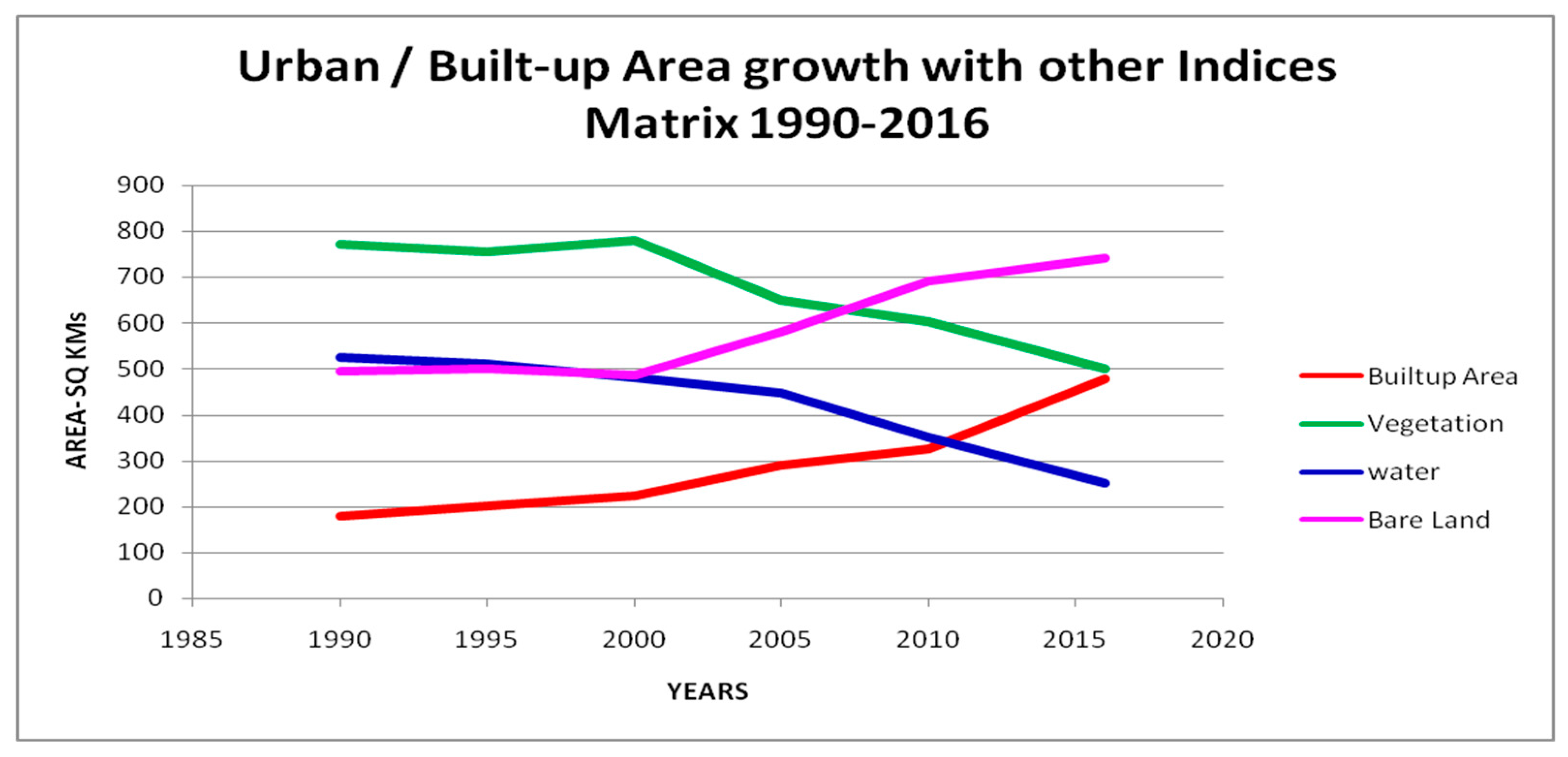
Table 3. Urban sprawl/built-up area growth with other Fields 1990–2016.
Name of Class19901995 2000 2005 2010 2016
Built-up Area (Sq. Km)178.74200222290325477
Bare Land (Sq. Km)494.83502.06487580.25690.99742
Vegetation (Sq. Km)770.75756780650.75602.33500
Water (Sq. Km)524.68510.94480448350.68250
Total196919691969196919691969
Table 4. (a) Points selected for accuracy assessment—1990. (b) Points selected for accuracy assessment—1995. (c) Points selected for accuracy assessment—2000. (d) Points selected for accuracy assessment—2005. (e) Points selected for accuracy assessment—2010. (f) Points selected for accuracy assessment—2016.
(a)
ClassClassification Fields—1990
WaterVegetationBuilt-Up AreaBare LandRow Total
Water4000444
Vegetation5350040
Urban/BU (Built-up) Area0037340
Bare Land0113436
Total Column45363841160
Producer’s Accuracy88.89%97.22%97.37%82.93%
User’s Accuracy90.91%87.5%92.5%94.44%
Overall Accuracy91.25%
Kappa Coefficient 0.883
(b)
ClassClassification Fields—1995
WaterVegetationBuilt-Up AreaBare LandRow Total
Water3800745
Vegetation6326044
Urban/BU (Built-up) Area2028737
Bare Land0003234
Total Column40353451160
Producer’s Accuracy79.17%100%82.35%69.57%
User’s Accuracy84.44%72.73%75.68%94.12%
Overall Accuracy81.25%
Kappa Coefficient 0.75
(c)
ClassClassification Fields—2000
WaterVegetationBuilt-Up AreaBare LandRow Total
Water3530038
Vegetation3420449
Urban/BU (Built-up) Area0050050
Bare Land0603238
Total Column38515036175
Producer’s Accuracy92.11%82.35%100%88.89%
User’s Accuracy92.11%85.71%100%84.21%
Overall Accuracy90.86%
Kappa Coefficient 0.88
(d)
ClassClassification Fields—2005
WaterVegetationBuilt-Up AreaBare LandRow Total
Water3000030
Vegetation5400247
Urban/BU (Built-up) Area0050353
Bare Land0003030
Total Column35405035160
Producer’s Accuracy85.71%100%100%85.71%
User’s Accuracy100%85.11%94.34%100%
Overall Accuracy93.75%
Kappa Coefficient 0.92
(e)
ClassClassification Fields—2010
WaterVegetationBuilt-Up AreaBare LandRow Total
Water3300235
Vegetation2320236
Urban/BU (Built-up) Area0048149
Bare Land0323540
Total Column35355040160
Producer’s Accuracy94.29%91.43%96%87.5%
User’s Accuracy94.29%88.89%97.96%87.5%
Overall Accuracy92.5%
Kappa Coefficient0.90
(f)
ClassClassification Fields—2016
WaterVegetationBuilt-Up AreaBare LandRow Total
Water2921032
Vegetation3310135
Urban/BU (Built-up) Area1148252
Bare Land1123741
Total Column34355140160
Producer’s Accuracy85.29%88.57%84.12%92.5%
User’s Accuracy90.63%88.57%92.31%90.24%
Overall Accuracy90.63%
Kappa Coefficient0.873
Publisher’s Note: MDPI stays neutral with regard to jurisdictional claims in published maps and institutional affiliations.

