Assessing CO₂ Emissions from Passenger Transport with the Mixed-Use Development Model in Shenzhen International Low-Carbon City

Abstract

Assessing transport CO₂ emissions is important in the development of low-carbon strategies, but studies based on mixed land use are rare. This study assessed CO₂ emissions from passenger transport in traffic analysis zones (TAZs) at the community level, based on a combination of the mixed-use development model and the vehicle emission calculation model. Based on mixed land use and transport accessibility, the mixed-use development model was adopted to estimate travel demand, including travel modes and distances. As a leading low-carbon city project of international cooperation in China, Shenzhen International Low-Carbon City Core Area was chosen as a case study. The results clearly illustrate travel demand and CO₂ emissions of different travel modes between communities and show that car trips account for the vast majority of emissions in all types of travel modes in each community. Spatial emission differences are prominently associated with inadequately mixed land use layouts and unbalanced transport accessibility. The findings demonstrate the significance of the mixed land use and associated job-housing balance in reducing passenger CO₂ emissions from passenger transport, especially in per capita emissions. Policy implications are given based on the results to facilitate sophisticated transport emission control at a finer spatial scale. This new framework can be used for assessing the impacts of urban planning on transport emissions to promote sustainable urbanization in developing countries.

1. Introduction

Reducing greenhouse gas (GHG) emissions as a response to climate change has been listed as part of the Sustainable Development Goals (SDGs) of the “2030 Agenda for Sustainable Development” set by the United Nations. The transport sector is a major contributor to GHG emissions, and the road transport sector alone accounted for 18.52% of the global GHG emission in 2016 [1,2]. In developed countries, this proportion could even be over 40% [3,4,5]. China is the country with the highest level of GHG emissions, and the transport sector accounted for 16.22% of the national total amount in 2016 [6]. Its carbon emission growth rate was 12.45% in 2007–2016, ranking first across all sectors [6]. CO₂ is the primary GHG in China [7], so controlling transport CO₂ emissions in China is important for the reduction of global GHG emissions. Urban passenger transport is increasingly contributing to CO₂ emissions [8], and to control these urban carbon emissions, the Chinese government has established multiple groups of pilot low-carbon cities since 2010, including some megacities such as Tianjin, Chongqing, Hangzhou, and Shenzhen. Reducing CO₂ emissions from urban passenger transport plays an important role in the development of low-carbon cities.

Estimating CO₂ emissions from passenger transport is the foundation for setting and achieving CO₂ reduction goals of low-carbon development. It is of utmost importance for cities to assess emissions at a finer scale in cities to provide a more scientific basis for addressing the issue. Land use has a decisive impact on the emissions of transport activities [9]. With the rapid urbanization process in developing countries, urban sprawl and unreasonable land use layouts have increased the overall travel distance of urban residents, stimulating travel demand and subsequent emissions [10]. To reduce the emissions by land use planning and to achieve sustainable urbanization, land use should be taken into consideration in the estimation of travel demand and the associated CO₂ emissions.

In this study, mixed land use and transport accessibility are taken into consideration to estimate travel demand with the mixed-use development model. CO₂ emissions from passenger transport in traffic analysis zones (TAZs) at the community level were assessed based on travel demand. As a leading low-carbon city area of international cooperation in China, Shenzhen International Low-Carbon City Core Area was chosen to be the study area to provide insight for global sustainable development. The purpose of this paper is to provide a new framework to estimate CO₂ emissions from passenger transport based on mixed land use and transport accessibility for providing a scientific tool of assessing and optimizing land use planning, which can be an important pathway for reducing CO₂ emissions from passenger transport and promoting sustainable urbanization.

The novelty of this study lies in assessing transport emissions at a finer spatial scale within a city, based on a combination of two models: the mixed-use development model and the vehicle emission calculation model. This study also estimated travel demand based on mixed land use and transport accessibility with the mixed-use development model. The research outcomes can provide reference for urban areas with limited traffic data to estimate passenger transport emissions more suitably, facilitating low-carbon transport strategies by optimizing land use and transport planning in a more sophisticated manner.

The remainder of the paper is organized as follows. In Section 2, previous studies are reviewed. In Section 3, the study area, ology, and data are described. In Section 4, the estimated results of the travel demand and CO₂ emissions from passenger transport in TAZs at the community level are assessed. Finally, a discussion, the conclusions, and policy implications are presented based on the results to facilitate low-carbon transport strategies.

2. Literature Review

For estimating carbon emissions from passenger transport, some studies have explored different methods, and these methods can be divided into three dominant categories: The first is based on energy consumption, and the methodology of the Intergovernmental Panel on Climate Change (IPCC) lies in this type [11]; the second is based on vehicles, and in this method vehicle emissions are calculated with the statistical data of the total vehicle ownership, population of each type of vehicles, average kilometers travelled by vehicles, fuel efficiency, and emission factors [12]; the third is based on traffic flows observed by monitoring devices or on-site surveys [13,14,15]. However, existing methods have their shortcomings despite their widespread use. First, these methods are mainly used for large-scale regions, and the related data are usually unavailable for a finer scale within a city. The methods based on fuel consumption or vehicles utilize the data mostly available only for large-scale regions or the entire city. Meanwhile, methods based on traffic flows can describe urban emission distribution, but the data are usually unavailable in many urban areas or are limited to individuals [16,17,18]. Second, these methods mainly focus on the role of fuels in transport emissions, but fuel improvement alone is not adequate to control emissions because of the sharp increase in the number of passenger vehicles [6].

In contrast, studies of the estimation of travel behaviors and related emissions from passenger transport based on land use are relatively rare despite the significant impacts that land use may have on travel demand emissions. A variety of human activities are distributed in different locations and land use types, which are the foundation of travel demand and transport activities that connect people [19]. Many studies have revealed that higher development densities [9], compact urban forms [20] and diverse land use layouts [21] may reduce travel demand and associated emissions. To estimate travel demand, some researchers have explored a few land use-based transport (LUT) models, and the LUT models for estimating travel demand can be classified into four types [22]. The first is the spatial interaction model, examples of which include the four-step trip-based model [23] and Lowry model [24]. The gravity model and the entropy model are adopted to estimate traffic flows between regions in these models. It is the most conventional and simple type [25]. The second is the spatial economic model, examples of which include the Tranus model [26] and the economic land use-transport (DELTA) model [27]. In these models, urban space is regarded as economic units with production and consumption activities, and traffic flows are estimated by the activity flows between locations. Some scholars have used the Tranus model to estimate the travel demand of large cities [28,29]. The third is the random utility and discrete choice model, examples of which include the micro-econometric land use and transport (METROSIM) model [30] and the UrbanSim model [31]. In these models, land location choice is taken into consideration to estimate related traffic flows [32]. The fourth is the micro-behavior model, an example being the integrated land use-transportation-environment (ILUTE) microsimulation model [33]. Individual travel-related micro-travel behaviors are mainly considered in these models.

Although there are some LUT models that estimate the travel demand, limitations still exist. First, the transport models mentioned above rarely consider the impact of mixed development on transport emission reduction. Mixed-use development is an urban land use pattern, and by allocating different land uses close to each other, this pattern creates chances of various activities like working and housing completed in the same place, so that trips can be shorter or inside one zone to reduce car dependency [34,35,36]. Second, the spatial scale is mostly focused on a large district of a city or a provincial region, only reflecting macro-spatial forms. However, travel behavior is often affected more by micro-land use, and detailed travel behavior data with geographic information are usually unavailable at the fine spatial scale [20]. Estimation of the spatial distribution of modal split ratios and emissions of different transport modes is still not very clear. Third, some models place a greater emphasis on socioeconomic variables and discount the effects of land use and transport accessibility.

Thus, it is necessary to adopt the mixed-use development model to overcome these shortcomings. This model is an LUT model for estimating travel demand that includes distances and modes with travel purposes. The mixed-use development model takes the reduction effects of mixed-use development on car trips into consideration [37,38]. Past studies have shown that the mixed-use development model has the advantage of reliable feasibility for estimating travel demand. The mixed-use development model has been adopted by public agencies in U.S. for transportation planning [39,40], and it was originally developed for the U.S. Environmental Protection Agency based on travel survey data in metropolitan regions. Since then, scholars have applied and improved this model [41,42], and related studies have indicated that the mixed-use development model is generally accurate and convincing in estimating travel demand of inhabitants [38,43].

However, only a limited number of studies have applied the mixed-use development model in practice. In particular, assessment of the spatial differences of travel demand at the community level has not been clear in previous studies. Therefore, it was necessary to apply the mixed-use development model in this assessment.

3. Material and Methodology

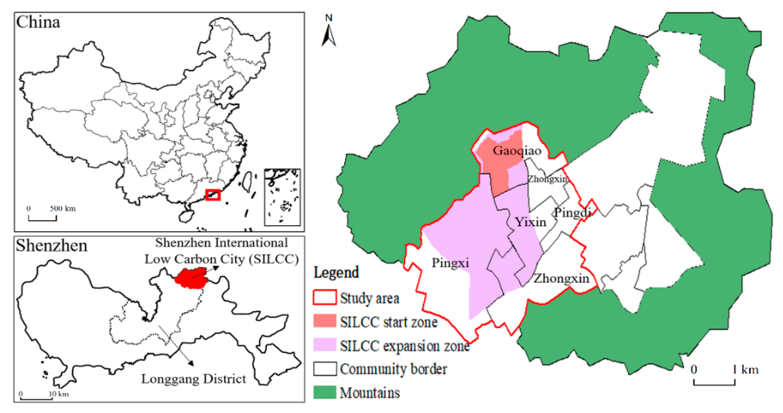
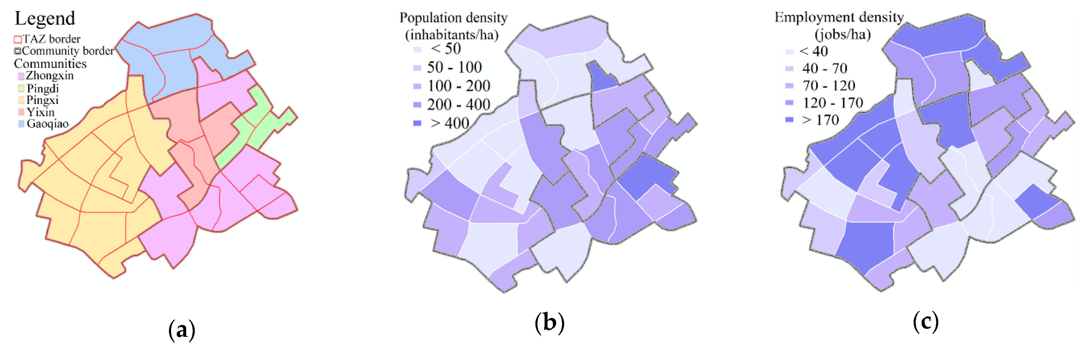
3.1. Study Area

As a growing megacity in the developed coastal region of China, Shenzhen is included in the national innovation-driven demonstration zones as part of China’s implementation of the SDGs. Shenzhen International Low-Carbon City (ILCC) is located at the northeast fringe of Shenzhen. Started in 2012, it is a flagship project for cooperation on sustainable urbanization between China and the European Union. This project aims to serve as an example to the rest of the world of the best practices of sustainable development. Its demonstration of low-carbon development has drawn international attention and has gained worldwide recognition. As a leading low-carbon development area of Shenzhen, it is necessary to reduce travel demand and transport emissions of the growing population of the area and to find innovative solutions for promoting low-carbon transport policies in ILCC.

The general planning extent of ILCC is the entire Pingdi subdistrict of the Longgang district, covering an area of 53.4 km². It consists of three parts, including the start zone, the expansion zone, and the remaining part. The start zone and the expansion zone are planned to be firstly developed in the entire area, involving 5 communities with more available data and most of the population and transport activities in the entire subdistrict. Therefore, these five communities were chosen to be the study area, which is considered as ILCC Core Area (Figure 1).

The study area covers 11.79 km² with a variety of urban land types, including employment and residential land. In terms of the urban passenger transport, the modes in the study area include buses, cars, and active modes. There were 23 bus routes with 188 bus vehicles serving the study area, and the bus route density was obviously uneven distributed (Figure 2). This distribution pattern indicated severe spatial inequalities of the level of integration of the passenger transport, requiring further optimization planning. To make planning and redevelopment more reasonable, it is necessary to estimate transport emissions for providing scientific reference.

3.2. Methodology

The methodology of this study was separated into three subsections. Section 3.2.1. describes the general framework for estimating CO₂ emissions from passenger transport; Section 3.2.2. explains how to estimate travel demand based on the mixed-use development model; Section 3.2.3. explains how to estimate carbon emissions from passenger transport with the output of Section 3.2.2.

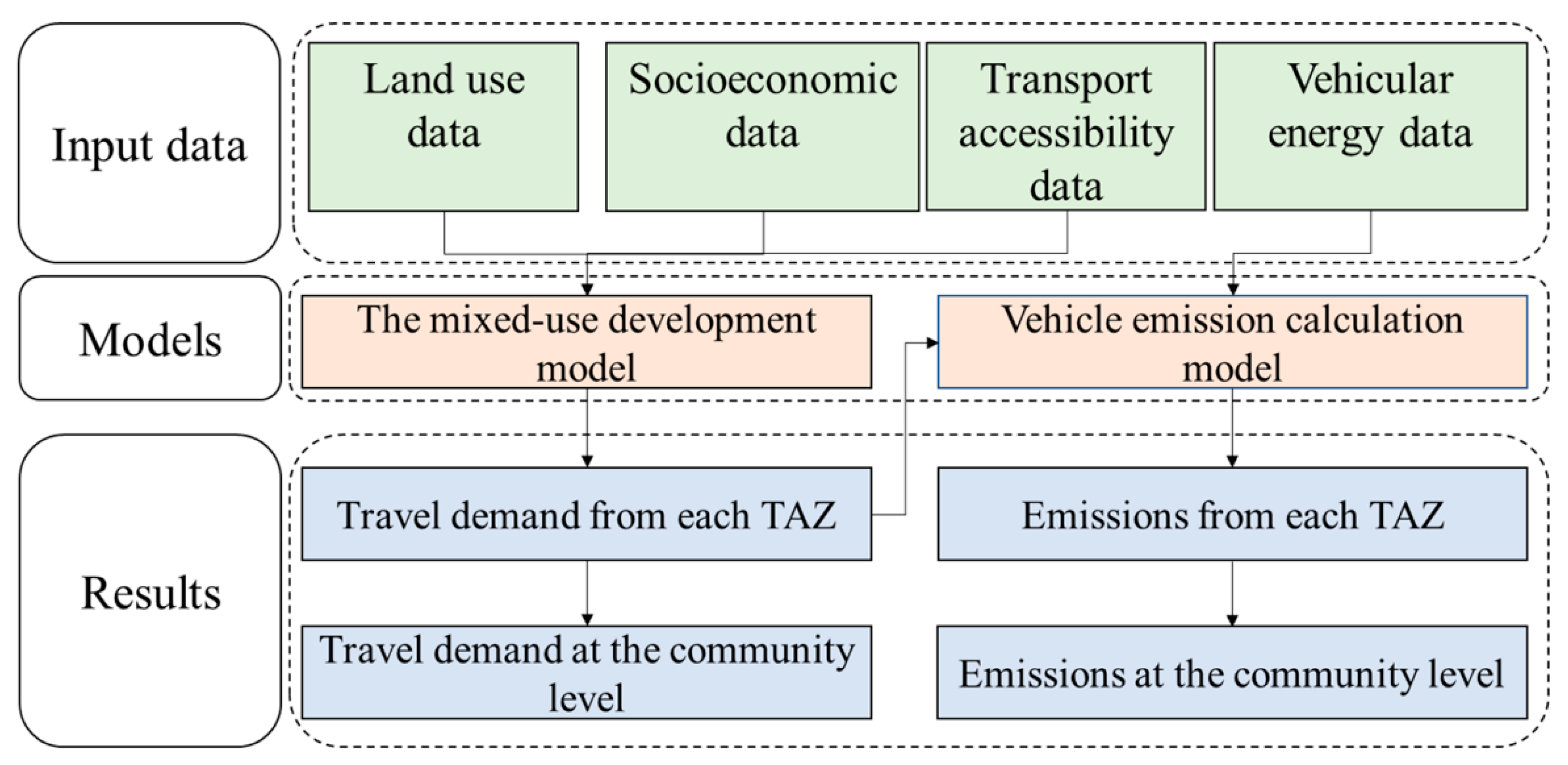
3.2.1. General Framework

The general framework of the research methodology of this study is presented in Figure 3. It shows the input data, calculation models, output results, and process flows. The framework includes two models, namely, the mixed-use development model and the vehicle emission calculation model. The mixed-use development model was adopted to estimate travel demand, and generated output data were employed to estimate CO₂ emissions from passenger transport with the vehicle emission calculation model. As a bottom-up method, the framework reflects the impact of travel behavior on transport emissions.

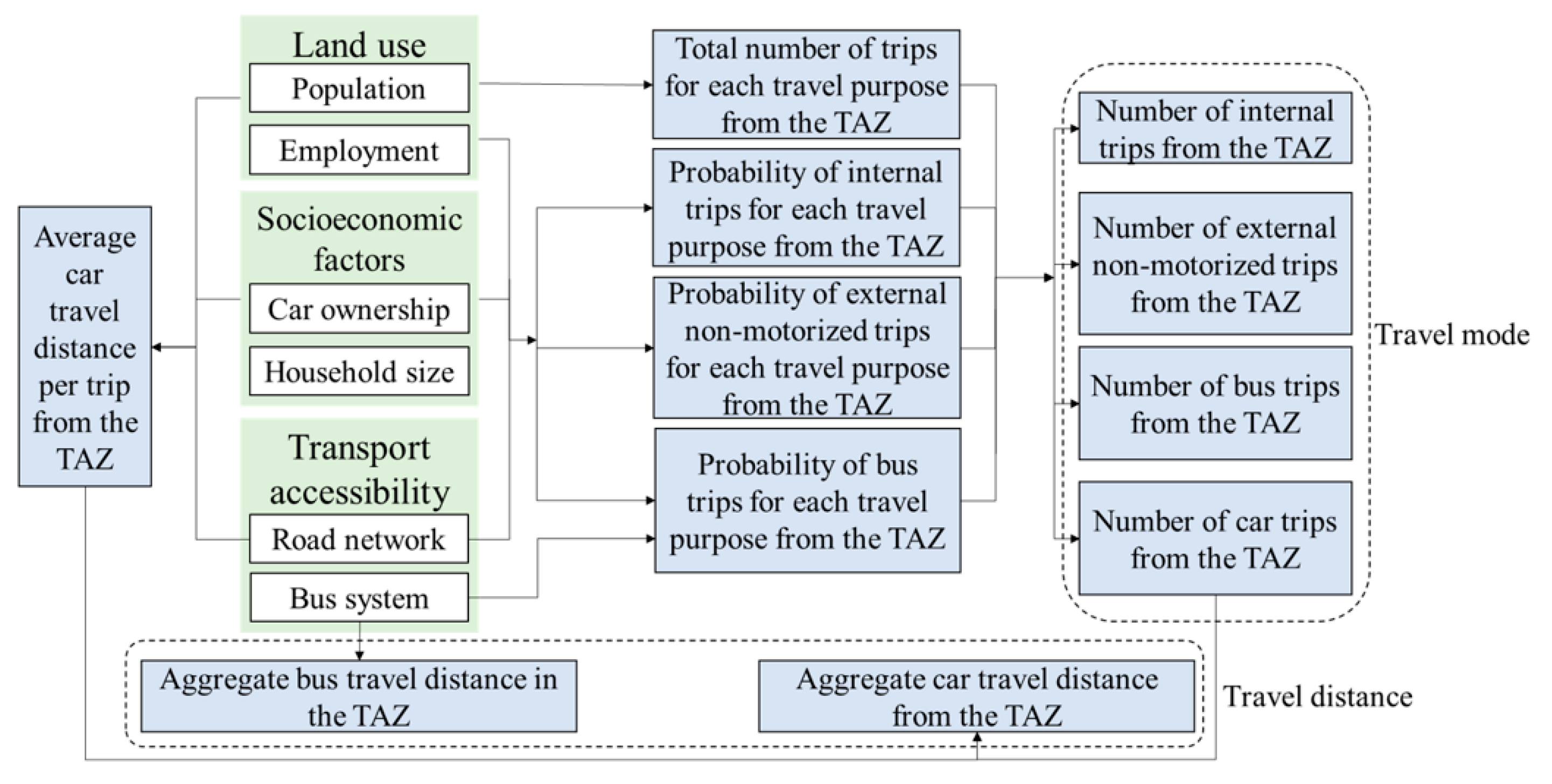
3.2.2. Travel Estimation Based on the Mixed-Use Development Model

The mixed-use development model was used to estimate the travel demand of each TAZ in the study area. Taking time of the day into consideration, this model is suitable for estimating the travel demand at the daily level as well as the morning or evening peak hour level based on the same framework with different coefficients. As shown in Figure 4, the input elements include three categories of parameters, namely, land use, socioeconomic factors, and transport accessibility. Based on travel purposes, the output elements for travel demand include two main categories, namely, travel modes and vehicle travel distances.

Travel modes were estimated as follows. First, the total number of trips from the TAZ was estimated with the improved Institute of Transportation Engineers (ITE) model, of which the original version was built by the ITE [44]. As indicated in previous studies, given that the original ITE model is not for smart-growth areas like areas that are purposefully designed to include mixed land uses and higher densities, the mixed-use development model has made adjustments to ITE trip rates to make them suitable for smart-growth areas. Scholars have used the mixed-use development model to quantify multimodal trip generation, including active trips and public transit trips. In this model, all modes are counted in generated trips, where active trips and transit trips are considered as the substitution for car trips in the mode choice impacted by land use and accessibility [35,37,38,41,45].

In the parameters mixed-use development model, parameters of the input elements were selected to estimate the probabilities of different travel modes, and these modes included internal trips, external active trips (i.e., walking and bicycles), and bus trips. The origin and destination of an internal trip should both be within the TAZ, and internal trips from the TAZ are in the active mode because of the small land area as restricted in the mixed-use development model. In this study, each TAZ is restricted to a land area smaller than 1 km², and the estimated maximum time a traveler might experience for an internal trip by waking and cycling may not exceed 20 min and 10 min, respectively, making active trips more convenient for travelers [46]. Therefore, bus trips and car trips were all defined as external trips. The travel purposes in the mixed-use development model were divided into three types, namely, home-based work trips, home-based other trips, and non-home-based trips. The time periods were also divided into three types, namely, daily period, morning peak period, and evening peak period. For each travel purpose and each type of time period, the number of trips for each travel mode excluding cars was calculated respectively with the total number and probability of trips. Finally, the number of car trips for each travel purpose was calculated with the number of total trips and other modes of trips. Cars included private cars and taxis. According to related research [37,38,41,47,48], the basic equations are:

$$T_{totaljwt}={\displaystyle \sum }_i{f}_{iwt}\left(X_{ij}\right)$$

(1)

$$p_{kjwt}=\exp \left(l{o}_{kjwt}\right)/\left(1+\exp \left(l{o}_{kjwt}\right)\right)$$

(2)

$$l{o}_{kjwt}=f_{kjwt}\left(variabl{e}_{k1wt},variabl{e}_{k2wt},\dots ,variabl{e}_{knwt}\right)$$

(3)

$$T_{kjwt}=T_{totaljwt}\times p_{kjwt}$$

(4)

$$T_{carjwt}=T_{totaljwt}-{\displaystyle \sum }_k{T}_{kjwt}$$

(5)

where T_totaljwt is the total number of trips from TAZ j for travel purpose w in time period t and X_ij is the amount of land type i in TAZ j (such as land area and number of units); the function f_iwt(X_ij) calculates the total trips of land type i from TAZ j for travel purpose w in time period t, and the specific calculation formulas can be found in the improved ITE model [44,45,47]; p_kjwt represents the probability of non-car trips by mode k from TAZ j for travel purpose w in time period t; lo_kjwt is the natural logarithm of the odds of non-car trips by mode k from TAZ j for travel purpose w in time period t; T_kjwt is the number of non-car trips by mode k from TAZ j for travel purpose w in time period t; T_carjwt is the total number of car trips from TAZ j for travel purpose w in time period t.

Based on the results of travel modes, the daily aggregate travel distances of cars and buses were estimated. The formulas are [48]:

$$L_{carj}={\displaystyle \sum }_w{T}_{carjw1}\times A{L}_{carjw}$$

(6)

$$L_{busj}=R{T}_{mj}\times Q{T}_{mj}$$

(7)

where L_carj is the daily aggregate travel distance of cars from TAZ j; AL_carjw is the daily average car travel distance per trip from TAZ j, calculated using the selected parameters in the input elements for travel purpose w; L_busj is the daily aggregate travel distance of buses in TAZ j; RT_mj is the length of bus route m in TAZ j, and QT_mj is the corresponding bus quantity; T_carjw1 is the total number of daily car trips from TAZ j for travel purpose w.

Specifically, lo_kjw of Equation (3) and AL_carjw of Equation (6) were calculated with input variables as shown in

Table 1. Variables of the input elements in the mixed-use development model.

Categories	Variables	Symbols
Land use	The amount of type i land in TAZ j	Xij
	The total land area of TAZ j	AEj
	The total number of jobs in TAZ j	REj
	The aggregate number of population and employment per unit area in TAZ j	DAj
	The integrated index of population and total employment in TAZ j	EPj
	The integrated index of population and commercial employment in TAZ j	CPj
Socioeconomic factors	Vehicle ownership per capita in TAZ j	VAj
	The household size in TAZ j	HSj
Transport accessibility	The number of jobs within a 1.6 km buffer outside the border of TAZ j	MEj
	Density of the intersections within TAZ j	INj
	The number of jobs accessible within a 30-min bus trip of TAZ j from the central point of TAZ j	BTRj
	The portion of jobs within a 30-min car trip of TAZ j in the study area from the central point of TAZ j	ATRj
	The portion of jobs within a 20-min car trip of TAZ j in the study area from the central point of TAZ j	ATWj

, and the specific formulas are [47,48]:

$$l{o}_{1jwt}={\beta }_{1wt}+{\displaystyle \sum }_i^n{\alpha }_{iwt}In\left(Variabl{e}_i\right),Variabl{e}_i=V{A}_j,I{N}_j,E{P}_j,H{S}_j,R{E}_j,A{E}_j$$

(8)

$$l{o}_{2jwt}={\beta }_{2wt}+{\displaystyle \sum }_i^n{\alpha }_{iwt}In\left(Variabl{e}_i\right),Variabl{e}_i=V{A}_j,I{N}_j,H{S}_j,D{A}_j,A{E}_j,E{P}_j,C{P}_j,M{E}_j$$

(9)

$$l{o}_{3jwt}={\beta }_{3wt}+{\displaystyle \sum }_i^n{\alpha }_{iwt}In\left(Variabl{e}_i\right),Variabl{e}_i=V{A}_j,I{N}_j,H{S}_j,R{E}_j,BT{R}_j$$

(10)

$$A{L}_{carjw}={\beta }_{4w}+{\displaystyle \sum }_i^n{\alpha }_{iw}In\left(Varibl{e}_i\right),Varibl{e}_i=I{N}_j,A{E}_j,V{A}_j,E{P}_j,AT{R}_j,AT{W}_j$$

(11)

where lo_1jwt, lo_2jwt, and lo_3jwt represent the natural logarithm of the odds of internal trips, external active trips, and bus trips from TAZ j for the travel purpose w in the time period t, respectively, and n represents the number of variables. The indications of variables in Variable_i are shown in Table 1; β_1wt, β_2wt, β_3wt, β_4w, α_iwt, and α_iw are correlation coefficients based on related studies [38,42,43,45,47,49].

As shown in Table 1, land use indicators of the density and mixed use are included in the input elements because of their importance in the mixed-use development model. For example, the aggregate number of population and employment per unit area is the indicator of the development density. This indicator directly shows the general density of human activities. Besides, the level of mixed land use is of great significance in this model, and it was measured by two integrated indices of population and employment in Table 1. The spatial mix level of residential and employment land can be quantified by the indices. The formulas are [47,48]:

$$E{P}_j=max\left(1-\frac{\left|0.2\times PO{P}_j-R{E}_j\right|}{0.2\times PO{P}_j+R{E}_j},0.01\right)$$

(12)

$$C{P}_j=max\left(1-\frac{\left|0.05\times PO{P}_j-C{E}_j\right|}{0.05\times PO{P}_j+C{E}_j},0.01\right)$$

(13)

where EPj is the integrated index of population and total employment in TAZ j; POP_j is the population in TAZ j; RE_j is the number of jobs in TAZ j; CP_j is the integrated index of population and commercial employment in TAZ j; CE_j is the number of commercial jobs in TAZ j. For total employment, different jobs are distributed in different types of land use. For commercial jobs, the model has a more detailed classification, including retail, supermarket, bank, restaurant, hotel, theater, and other commercial activities. The number of jobs is calculated based on the employment density and land amount [47,48].

3.2.3. Vehicle Emission Calculation Model

After estimating travel demand in the mixed-use development model, its output results for the travel distance of each vehicle type were used to calculate CO₂ emissions based on the vehicle emission calculation model [50]. The passenger vehicles in the study area can be divided into two categories, namely, cars and buses. The parameters of vehicular energy in this model are shown in

Table 2. Parameters of vehicular energy in International Low-Carbon City (ILCC) Core Area in 2016.

Vehicle Type	Energy Type	Energy Proportion (%)	Energy Intensity (kgce/km)	Emission Factor (kgCO2/kgce)
Cars	Gasoline	99.77	0.08	2.08
	Electricity	0.23	0.02	1.42
Buses	Electricity	100.00	0.13	1.42

.

3.3. Data Sources

The field investigation of the study area was carried out to collect the basic data demanded by this study. The authors also visited authorities and research institutes associated with the study issues in Shenzhen for data preparation. Statistical reports, literature, and other online resources were also investigated to acquire related data.

The values of the input variables in the models were obtained by processing the data collected from the investigation. These variables were divided into four categories, namely, vehicular energy, land use, socioeconomic factors, and transport accessibility. The vehicular energy data were from related studies [51,52] and Longgang Transport Administration. The land use data were from Pingdi Subdistrict Administration, Longgang Land Administration, Urban Planning & Design Institute of Shenzhen, and Shenzhen Bureau of Statistics. The numbers of employment and population were calculated based on land use [47,48]. The socioeconomic data were from Shenzhen Bureau of Statistics and Pingdi Subdistrict Administration. As for the transport accessibility data, the data of the transport facilities were from Longgang Transport Administration, and the numbers of jobs accessible for different modes were calculated using the ArcGIS software with the data of both transport facilities and employment land.

For more accurate analysis, the study area was subdivided into individual TAZs. The zoning was in accordance with the following principles. First, the land area of a TAZ is restricted to 388.50 ha or smaller, and there should be no major roads crossing the interior of a TAZ in the mixed-use development model [48]. Thus, internal trips in a TAZ can be easily completed by active modes, such as walking, so that car trips are only necessary for external trips [36]. If a TAZ is too large, some internal trips might not be active trips. Second, local geographic factors should be taken into consideration in zoning. Major rivers and administrative borders of communities should not cross the interior of a TAZ, given the spatial accessibility and community statistics. Third, the land areas of TAZs should be allocated as proximate as possible to make them more comparable at the spatial scale.

4. Results

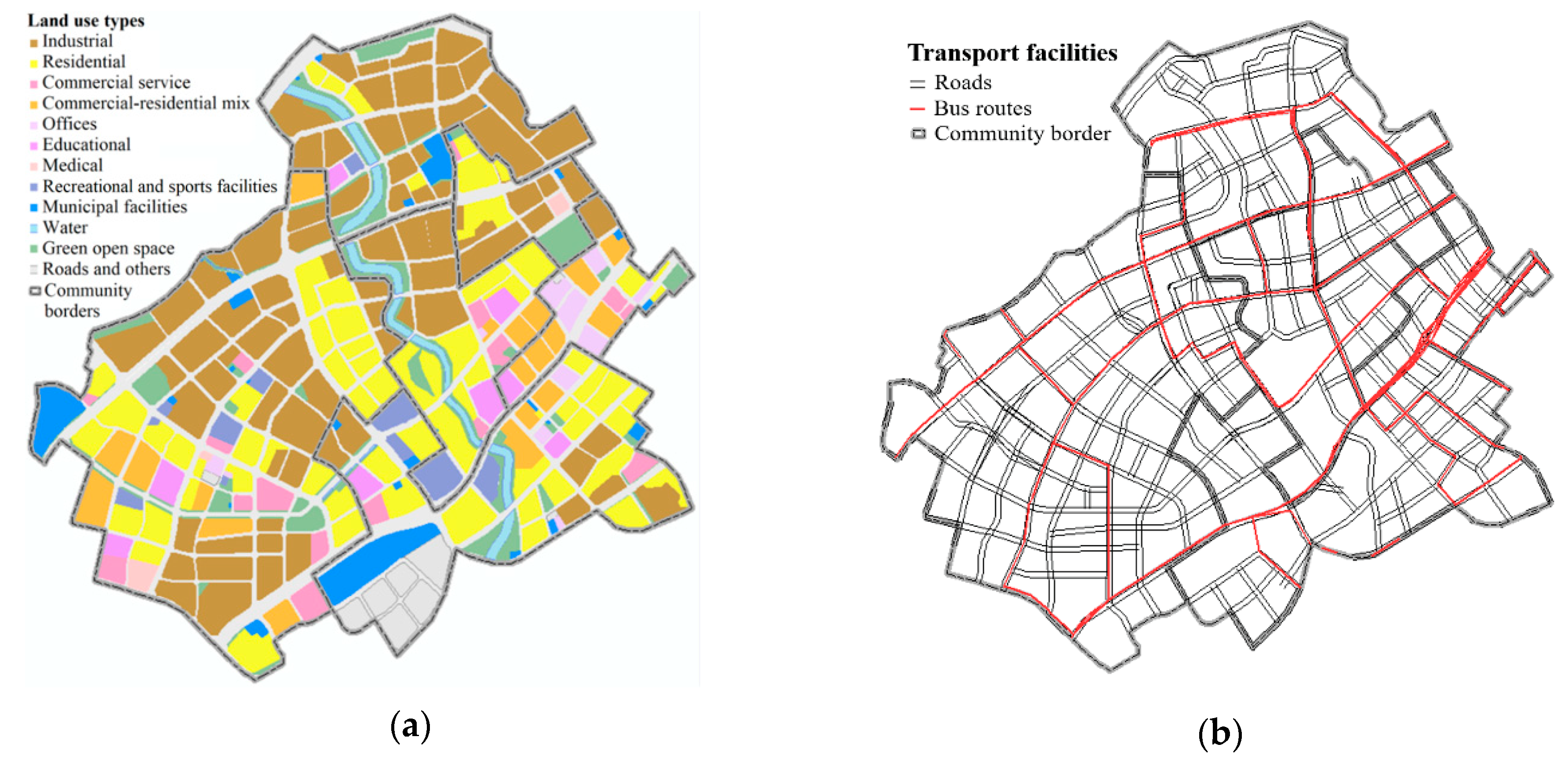
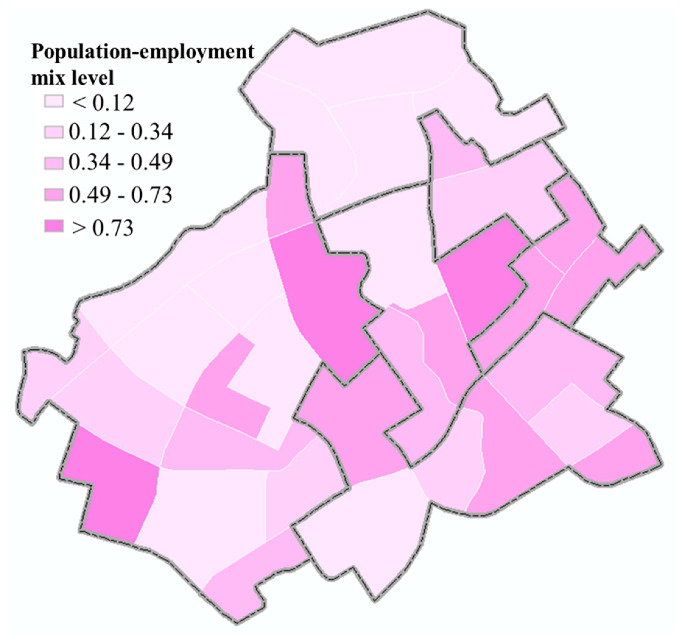
4.1. Land Use Analysis

Based on the zoning principles in Section 3.3, the five communities of the study area were subdivided into a total of 34 TAZs, as shown in Figure 5a. Therefore, each community contained at least a few TAZs.

Based on the types and amount of different land uses with different population and employment densities, spatial density distribution patterns of population and employment were calculated and are presented in Figure 5b,c, respectively. According to the calculated results, the TAZs with higher population densities are mainly distributed in the southern and eastern parts of the study area. This is because most residential land is concentrated in these TAZs, in which most people live in. Especially in the southeast, five TAZs account for 24.48% of the residential land in the whole study area, while their total land area only takes up 12.11%, showing a very highly concentrated population distribution pattern. However, the spatial density distribution pattern of employment is quite different from that of the population. Most of the TAZs with higher employment densities are distributed in the northern and western parts, where industrial land that can provide plenty of job opportunities is the land type accounting for the largest proportion. By comparing Figure 5b,c, a severe spatial imbalance between residence and employment can be observed. This imbalanced spatial form may play an important role in the generation of travel demand and associated transport emissions.

4.2. Travel Demand Analysis

Based on the estimated results of the TAZs from the mixed-use development model, the travel demand of each community in the ILCC Core Area was summarized.

Table 3. Estimated annual travel demand of the ILCC Core Area in 2016.

Indicators			Communities					Overall
			Gaoqiao	Pingdi	Pingxi	Yixin	Zhongxin
Travel modes	Total trips (million)		21.59	42.78	86.64	25.96	65.50	432.24
	Modal distribution of internal trips (%)		7.53	8.65	8.17	7.95	5.98	7.39
	Modal distribution of external trips (%)	External active trips	30.99	31.47	29.70	25.15	22.15	26.95
		Car trips	53.07	51.87	55.94	61.32	67.23	59.57
		Bus trips	8.40	8.00	6.17	5.58	4.64	6.09
Travel distances	Car travel distances (108 km)		0.95	1.38	4.38	1.16	2.77	10.64
	Bus travel distances (105 km)		1.75	4.12	6.53	3.49	6.31	22.20

demonstrates the results of the travel modes and vehicle travel distances, as well as a few differences between communities. The indicators were analyzed more closely as follows.

In the total trips, car trips have the highest modal split ratio in each community, followed by external active trips. This indicates that the travel modes are dominated by cars, and the low-carbon transport system still requires improvement. As the study area is a suburban area, its public transport services are still inadequate, and people may have to use cars to reach their destinations much faster, especially when covering a long or medium distance. People tend to use active modes instead of buses on external trips without cars. Trips within a short distance could be more conveniently made by walking or taking a bicycle than waiting for a bus. Moreover, the modal split ratio is low for all internal trips, suggesting that in most TAZs, people can hardly meet their travel demands within the TAZ they are located in, indicating that the internal land diversity is mostly low and that mixed-use development is not evenly distributed. As for travel distances, differences at the community level show that a community with a higher modal split ratio of bus trips is expected to have a shorter car travel distance. However, some communities with longer bus travel distances have lower bus trip modal split ratios. This implies that the public transport system is not significantly effective in reducing the number of car trips when associated with unsuitable land use layouts.

The distribution patterns of travel purposes are quite different for all the modes at the community level (

Table 4. Estimated distribution patterns of travel purposes of the ILCC Core Area in 2016.

Trip Proportions of Travel Purposes (%)		Communities					Overall
		Gaoqiao	Pingdi	Pingxi	Yixin	Zhongxin
Total trips	Home-based work	40.97	30.51	33.91	32.89	32.74	33.52
	Home-based other	34.48	41.67	39.90	41.38	41.76	40.38
	Non-home-based	24.55	27.82	26.19	25.73	25.50	26.10
Internal trips	Home-based work	60.17	45.28	52.85	47.58	47.32	49.70
	Home-based other	17.89	31.22	29.01	35.32	33.80	30.60
	Non-home-based	21.94	23.49	18.14	17.10	18.88	19.69
External active trips	Home-based work	63.92	44.14	48.97	51.56	45.02	48.60
	Home-based other	34.00	50.11	48.29	45.98	51.91	48.03
	Non-home-based	2.08	5.75	2.75	2.47	3.07	3.36
Car trips	Home-based work	25.58	19.05	25.13	28.88	27.79	26.03
	Home-based other	35.02	36.78	37.82	36.07	31.96	35.78
	Non-home-based	39.40	44.18	37.05	35.05	40.25	38.19
Bus trips	Home-based work	22.41	35.18	19.29	13.11	10.49	20.36
	Home-based other	67.00	51.54	64.42	68.40	69.47	63.52
	Non-home-based	10.59	13.28	16.29	18.49	20.05	16.12

). As an employment center, the proportions of the home-based work purpose for total trips and internal trips in the Gaoqiao community are both the highest, indicating the concentration of employment land. The proportions of the non-home-based purpose are both the highest for total trips and internal trips in the Pingdi community, resulting from the agglomeration of commercial land and various services. The highest proportions of the home-based other purpose for total trips and internal trips are both in the southern communities such as Yixin and Zhongxin, where residential land is largely concentrated. The characteristics of travel purposes for external active trips are generally similar to that of internal trips. The proportion of the home-based work purpose for car trips is the lowest in the Pingdi community compared with other communities while it is the highest for bus trips because of the densely distributed bus routes and better transport accessibility. In contrast, the proportions of the home-based work purpose for car trips in the southern communities are much higher while these proportions are much lower for bus trips. In all communities, the proportions of the home-based work purpose are much lower than that of the home-based other purpose for bus trips. This shows that the allocation of bus routes is not suitable for meeting the commuting travel demand and reducing the car dependency.

In terms of the daily time periods, the differences of the trip numbers in different time periods of a day, especially peak hours, are prominent for the modes and communities (

Table 5. Estimated trips in different time periods of the ILCC Core Area in 2016.

Trip Proportions of Time Periods (%)		Communities					Overall
		Gaoqiao	Pingdi	Pingxi	Yixin	Zhongxin
Total trips	Morning peak	11.88	8.57	9.15	9.25	8.97	9.25
	Evening peak	12.64	12.53	12.10	13.06	9.72	11.69
	Other	75.48	78.91	78.75	77.69	81.31	79.06
Internal trips	Morning peak	14.14	10.36	11.02	10.41	10.91	11.07
	Evening peak	13.80	13.30	12.69	13.20	10.10	12.20
	Other	72.06	76.34	76.29	76.38	78.99	76.73
External active trips	Morning peak	15.55	11.06	11.54	11.11	11.21	11.71
	Evening peak	13.43	12.63	12.60	12.93	9.70	11.86
	Other	71.02	76.31	75.86	75.96	79.09	76.43
Car trips	Morning peak	8.52	8.41	9.91	11.89	18.82	12.58
	Evening peak	13.25	12.36	12.41	11.98	9.79	11.66
	Other	78.23	79.22	77.68	76.13	71.39	75.76
Bus trips	Morning peak	10.56	11.73	9.28	8.69	7.85	9.56
	Evening peak	10.15	12.35	9.69	11.26	10.73	10.53
	Other	79.29	75.92	81.02	80.05	81.42	79.91

). For total trips and internal trips, the trip proportions of morning peak hours in the Gaoqiao community are both the highest, associated with the travel purpose of commuting to this employment center. The characteristics of trip proportions of time periods for external active trips are generally similar to that of internal trips. For car trips, the proportions of morning peak hours are obviously higher in the southern communities, while for bus trips these proportions are lower. The level of employment accessibility by bus trips are lower in these communities, and the inhabitants living there tend to use cars to reach their workplaces faster during the morning peak hours. The proportions of evening peak hours are apparently higher than that of morning peak hours for the bus trips in the southern communities, indicating more travel demand for non-commuting purposes.

To further analyze the impact factors on travel demand, the indicators of transport accessibility based on the average of TAZ calculation results are summarized in

Table 6. Transport accessibility in the ILCC Core Area in 2016.

Indicators	Communities					Overall
	Gaoqiao	Pingdi	Pingxi	Yixin	Zhongxin
Intersection densities (number/ha)	0.05	0.22	0.06	0.08	0.07	0.07
Average accessible employment by internal trips (104 jobs)	0.84	0.24	0.47	0.39	0.25	0.44
Average accessible employment by external active trips within 1.6 km (104 jobs)	8.92	11.99	8.74	7.32	7.26	8.85
Average accessible employment by bus trips within 30 min (104 jobs)	12.19	9.47	9.26	7.41	7.35	9.14

. For intersection densities, the Pingdi community, which has the highest average intersection density also has the highest modal split ratios of both internal trips and external active trips, suggesting that a denser road network may increase the accessibility of active trips, as well as the modal split of this mode. In terms of the amount of accessible employment, jobs that can be reached by internal trips are much fewer than those by external trips. The higher modal split ratio of bus trips is associated with a larger accessible employment in this mode. Communities in the north and east have better employment accessibility, not only because of the agglomeration of the TAZs with high employment density, but also because of the greater number of bus routes passing through. Hence, more accessible employment can generally increase the modal split of non-car trips.

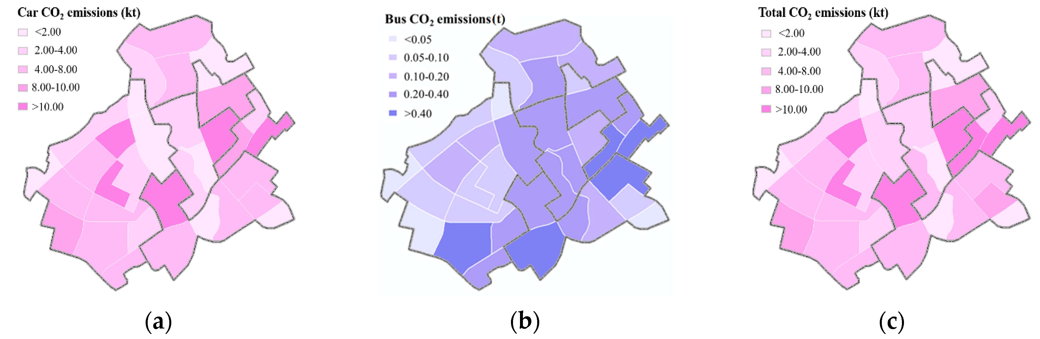
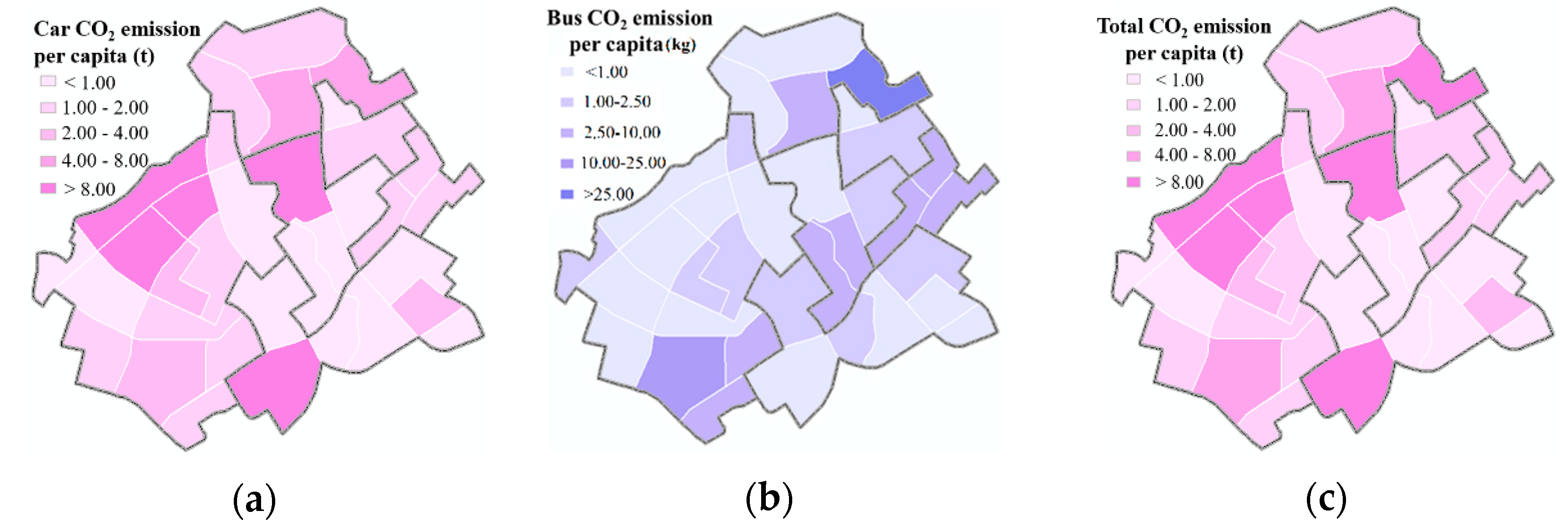
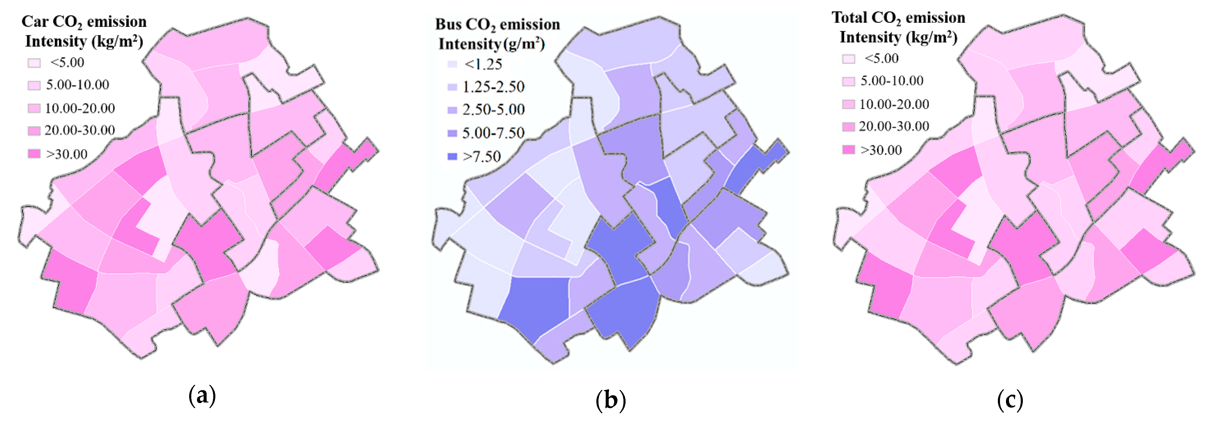
4.3. Transport CO₂ Emission Analysis

With the results of the travel demand analysis, the CO₂ emissions from the passenger transport of different communities were estimated based on the vehicle emission calculation model. As shown in

Table 7. Estimated CO₂ emissions from the passenger transport of ILCC Core Area in 2016.

Emission Indicators	Modes	Communities					Overall
		Gaoqiao	Pingdi	Pingxi	Yixin	Zhongxin
Total amount of CO2 emissions (kt)	Cars	15.76	22.98	72.74	19.34	45.95	176.77
	Buses	0.03	0.07	0.12	0.06	0.11	0.39
	Total	15.79	23.05	72.86	19.40	46.06	177.16
CO2 emissions per capita (kg)	Cars	4650.49	1179.69	32,543.34	35,267.06	22,175.83	24,085.87
	Buses	1.53	6.59	2.19	3.59	1.56	2.09
	Total	4652.02	1186.28	32,545.53	35,270.65	22,177.39	24,087.96

, the total CO₂ emissions from cars are much higher than that from buses in all communities. The differences of total CO₂ emissions between communities are due to the emissions from cars. Although the travel distances of cars are generally shorter than those of buses, the CO₂ emissions per capita of cars are significantly higher than that of buses for each community in the study area. Therefore, car trips are likely responsible for elevating the amount of emissions.

To further assess the differences in the amount of emissions at a finer scale, the spatial distribution patterns of the sources of the emissions are presented in Figure 6 and Figure 7. As Figure 6 shows, the sources from the passenger transport of the TAZs vary significantly across the study area. The total amount of emissions from the commercial and administrative centers in some of the east TAZs are much higher than that from most other TAZs. This is explained by the fact that the population in these centers is highly concentrated, and there are more vehicle trips from these TAZs. Some peripheral TAZs have a lower level of total emissions, which may be the result of their lower population. The distribution of bus emissions shows a center–periphery form, where the amount decreases from downtown to the surrounding areas. The amount of bus emissions is related to the distribution of the population and major roads. However, car emissions and total emissions have more dispersed spatial distribution patterns. Bus emissions in some central TAZs are low, implying fewer bus services, which result in people in these TAZs using cars on more trips. This shows that bus routes may not perfectly match the distribution of land use and travel demand.

The spatial distribution patterns of the sources of the per capita emissions of each TAZ are shown in Figure 7. People traveling from TAZs with lower values of per capita emissions show they have low emissions on their trips. Total emissions per capita in the eastern downtown center are lower than those in the north and southwest TAZs because of more mixed land use and better access to the public transport system. People in relatively less-mixed and lower-density TAZs in the southwest and northeast fringe tend to use cars to travel further to the center for commuting or other travel purposes. These findings indicate that different diversities of land uses can influence transport carbon production, especially per capita emissions. This connection is explicitly demonstrated in Figure 8, which displays the integrated index of population and total employment for each TAZ based on Formula (11). A higher value of this index means a higher mix level of land use. Comparing Figure 7 and Figure 8, it is clear that TAZs with higher values for the mix level of land use tend to have much lower per capita emissions because of more balanced job-housing distribution patterns. People in these TAZs can meet their travel demand more easily by non-car trips, making a great contribution to the decrease of individual transport emissions.

In addition to the amount, it is also important to assess the intensity of the transport emissions of each TAZ (Figure 9). This intensity is the emission level per unit area. The spatial distribution of the intensity of emissions is quite similar to that of the amount of emissions, but the differences between TAZs are even more prominent. The intensity of the emissions of southern and western TAZs is much higher than that of northern ones. This is likely to be an outcome of the densification of the residential population and commercial services, as well as the associated increase in transport emissions in these TAZs. In some central TAZs, the intensity of the emissions of buses is higher, while that of cars is low. However, in some western TAZs, it is the opposite, and in some southeast TAZs, both intensities are very high, indicating the emission reduction potential of bus routes and the inadequacy of public transport in the west.

As land use layouts are quite different between the communities, it is necessary to assess population- and employment-weighted emission intensities based on land use. As shown in

Table 8. Population- and employment-weighted emission intensities.

Emission Intensities (g/m2)	Modes	Communities					Average
		Gaoqiao	Pingdi	Pingxi	Yixin	Zhongxin
Population-weighted	Cars	373.18	1553.74	4242.29	2351.77	6144.53	2936.60
	Buses	1.02	3.55	9.86	5.13	13.49	6.28
	Total	374.20	1557.29	4252.15	2356.90	6158.02	2942.88
Employment-weighted	Cars	4133.77	3011.57	3544.80	1825.97	2478.87	2993.99
	Buses	8.64	6.59	8.22	4.10	5.19	6.81
	Total	4142.41	3018.16	3553.02	1830.07	2484.06	3000.80

, communities with higher employment-weighted emission intensities tend to have obviously lower population-weighted emission intensities. The average level of employment-weighted emission intensities is higher than the population-weighted level. This reveals the inequity issue of these communities. The level of mixed-use development in the study area is very low, and employment and residential land have a severely unbalanced distribution, resulting in a severe job-housing imbalance at the spatial level. This could result in people traveling to other communities for work or to acquire daily services, and cars are the travel mode much more convenient. Inequalities in land use have formed uneven spatial patterns of population and employment, resulting in a very high level of external travel demand. Meanwhile, unmatched bus routes drive people to use private travel modes, increasing car usage and associated emissions, especially for long or medium distances.

4.4. Uncertainties and Limitations

There are some uncertainties and limitations associated with the mixed-use development model when estimating travel demand, especially the car travel distance. There is randomness in individual travel behaviors, which are affected not only by land use, but also by their personal characteristics. For example, the individual preference of travel behaviors could be influenced by the age, gender, profession, income, family, educational background, and property ownership [53,54]. The remaining uncertainties due to different travel speeds and driving styles as well as vehicle conditions were excluded in this study. The data of some variables, such as vehicle ownership, are from statistical data on average, which might not be the same as the individual. Meanwhile, there are some uncertainties in the energy efficiency and emission factors of vehicles because of the difference of vehicle types, and these parameters adopted in this study is based on the average level. Due to this data limitation, it is impossible to know the detail of each person’s travel process and corresponding emissions, and uncertainties exist in this model. More surveys should be conducted in the mixed-use development model in future studies.

5. Conclusions and Policy Implications

5.1. Conclusions

Reducing transport carbon emissions is crucial for coping with climate change and for achieving sustainable development in many developing countries [55]. More sophisticated emission assessments and better urban planning may be important in achieving low-carbon goals. This study assessed CO₂ emissions from passenger transport in TAZs at the community level based on a combination of the mixed-use development model and the vehicle emission calculation model. The mixed-use development model was adopted to estimate travel demand, including travel modes and distances based on mixed land use and transport accessibility. As a leading low-carbon city project of international cooperation in China, Shenzhen International Low-Carbon City Core Area was chosen as a case study for assessment.

The results clearly illustrate CO₂ emissions of different passenger vehicle types and their spatial differences associated with land use layouts. Car trips account for the vast majority of emissions in all types of travel modes in each community, and although the total travel distance of cars is shorter than that of buses, cars are the largest CO₂ emission source of all forms of passenger transport. At the community level, spatial inequalities of travel demand and transport emissions are very prominent. Land use layouts on a small spatial scale may have a significant impact on travel behaviors, which directly determine the transport energy consumption and emissions.

The mixed land use and transport facilities are very inadequate in the study area, resulting in the decrease of low-emitting trips. Mixed land use may play an important role in reducing passenger CO₂ emissions from passenger transport, especially in per capita emissions. Employment land and residential land are unevenly distributed, resulting in a severe job-housing imbalance, and the bus routes are not well coordinated with land use and travel demand. The travel purposes and the trip proportions of peak hours are also impacted by the distribution patterns of residential and employment land. The job-housing imbalance and unreasonable transport facilities may decrease the commuting travel demand by buses. These unreasonable spatial attributes have caused severe inequalities of travel accessibility in the areas, leading to low modal split ratios of internal and bus trips. The analysis shows that a higher job-housing balance level may significantly reduce per capita transport emissions.

In general, the unreasonable allocation of land use layout and transport facilities have largely increased the high-emitting travel behaviors and spatial inequalities in developing urban areas. Therefore, more supporting options for low-carbon transport policy-making should be presented to reduce transport emissions.

5.2. Policy Implications

Based on the results of this study, several policy implications for improving low-carbon transport strategies can be highlighted as follows.

First, the low-carbon transport policy system should take the land use pattern and travel behaviors into consideration, given that land use may have significant impacts on travel behaviors. According to this study, the land use pattern of mixed-use development will improve land use diversity, which can significantly increase low-carbon travel behaviors of inhabitants to reduce high-emitting trips. The land use planning should reduce spatial equalities and control the development density properly.

Second, the planning of transport facilities, such as bus routes, should not only consider the population density, but should also pay attention to land use and inhabitants’ specific travel demand based on travel purposes to increase the user choices and modal split ratio of bus trips. To make car trips less necessary for traveling, suitable transit corridor should be established based on land use and actual travel demand for achieving the job-housing balance on the corridors and increasing the modal split ratio of bus trips, especially during the peak hours when the time is limited for commuting purposes.

Moreover, transport carbon emission inventories of communities in urban areas should be widely established for many countries where urbanization is developing rapidly. To implement low-carbon strategies in a more sophisticated manner, it is necessary to overcome data barriers and develop a better understanding of emissions at a finer scale, especially for less-developed countries. The mixed-use development model can be adopted for establishing transport emission inventories of current situations and future scenarios in small-scale urban areas. Such assessment can be used for evaluating the reduction in transport emissions of land use optimization policies to promote sustainable urbanization.

References

1. International Energy Agency (IEA). Key World Energy Statistics 2018; International Energy Agency (IEA): Paris, France, 2018.
2. International Energy Agency (IEA). World Energy Outlook; International Energy Agency (IEA): Paris, France, 2018.
3. International Energy Agency (IEA). World Energy Outlook 2017; International Energy Agency (IEA): Paris, France, 2017.
4. International Energy Agency (IEA). CO2 Emissions from Fuel Combustion 2011; OECD Publishing: Paris, France, 2011.
5. Muntean, M.; Guizzardi, D.; Schaaf, E.; Crippa, M.; Solazzo, E.; Olivier, J.G.J.; Vignati, E. Fossil CO2 Emissions of all World Countries-2018 Report; Publications Office of the European Union: Luxembourg, 2018. [Google Scholar]
6. National Bureau of Statistics. China Energy Statistical Yearbook-2017; China Statistics Press: Beijing, China, 2017. (In Chinese)
7. Wang, B.; Sun, Y.; Chen, Q.; Wang, Z. Determinants analysis of carbon dioxide emissions in passenger and freight transportation sectors in China. Struct. Chang. Econ. Dyn. 2018, 47, 127–132. [Google Scholar] [CrossRef]
8. Li, X.; Yu, B. Peaking CO2 emissions for China’s urban passenger transport sector. Energy Policy 2019, 133, 110913. [Google Scholar] [CrossRef]
9. Stanley, J.; Ellison, R.; Loader, C.; Hensher, D. Reducing Australian motor vehicle greenhouse gas emissions. Transp. Res. Part A Policy Pr. 2018, 109, 76–88. [Google Scholar] [CrossRef]
10. Kruszyna, M.; Śleszyński, P.; Rychlewski, J. Dependencies between Demographic Urbanization and the Agglomeration Road Traffic Volumes: Evidence from Poland. Land 2021, 10, 47. [Google Scholar] [CrossRef]
11. Solaymani, S. CO2 emissions patterns in 7 top carbon emitter economies: The case of transport sector. Energy 2019, 168, 989–1001. [Google Scholar] [CrossRef]
12. Tan, X.; Yuan, Z.; Gu, B.; Wang, Y.; Xu, B. Scenario Analysis of Urban Road Transportation Energy Demand and GHG Emissions in China—A Case Study for Chongqing. Sustainability 2018, 10, 2033. [Google Scholar] [CrossRef] [Green Version]
13. Espinosa, S.I.; Ynoue, R.Y.; Ropkins, K.; Zhang, X.; De Freitas, E.D. High spatial and temporal resolution vehicular emissions in south-east Brazil with traffic data from real-time GPS and travel demand models. Atmos. Environ. 2020, 222, 117136. [Google Scholar] [CrossRef]
14. Kholod, N.; Evans, M.H.; Gusev, E.P.; Yu, S.; Malyshev, V.L.; Tretyakova, S.; Barinov, A. A methodology for calculating transport emissions in cities with limited traffic data: Case study of diesel particulates and black carbon emissions in Murmansk. Sci. Total. Environ. 2016, 547, 305–313. [Google Scholar] [CrossRef] [Green Version]
15. Czepkiewicz, M.; Ottelin, J.; Ala-Mantila, S.; Heinonen, J.; Hasanzadeh, K.; Kyttä, M. Urban structural and socioeconomic effects on local, national and international travel patterns and greenhouse gas emissions of young adults. J. Transp. Geogr. 2018, 68, 130–141. [Google Scholar] [CrossRef]
16. Arioli, M.S.; D’Agosto, M.D.A.; Amaral, F.G.; Cybis, H.B.B. The evolution of city-scale GHG emissions inventory methods: A systematic review. Environ. Impact Assess. Rev. 2020, 80, 106316. [Google Scholar] [CrossRef]
17. Nocera, S.; Ruiz-Alarcón-Quintero, C.; Cavallaro, F. Assessing carbon emissions from road transport through traffic flow estimators. Transp. Res. Part C Emerg. Technol. 2018, 95, 125–148. [Google Scholar] [CrossRef]
18. Keall, M.; Shaw, C.; Chapman, R.; Howden-Chapman, P. Reductions in carbon dioxide emissions from an intervention to promote cycling and walking: A case study from New Zealand. Transp. Res. Part D Transp. Environ. 2018, 65, 687–696. [Google Scholar] [CrossRef]
19. Shabanpour, R.; Javanmardi, M.; Fasihozaman, M.; Miralinaghi, M.; Mohammadian, A. Investigating the applicability of ADAPTS activity-based model in air quality analysis. Travel Behav. Soc. 2018, 12, 130–140. [Google Scholar] [CrossRef]
20. Namdeo, A.; Goodman, P.; Mitchell, G.; Hargreaves, A.J.; Echenique, M. Land-use, transport and vehicle technology futures: An air pollution assessment of policy combinations for the Cambridge Sub-Region of the UK. Cities 2019, 89, 296–307. [Google Scholar] [CrossRef]
21. Guzman, L.A.; Peña, J.; Carrasco, J.-A. Assessing the role of the built environment and sociodemographic characteristics on walking travel distances in Bogotá. J. Transp. Geogr. 2020, 88, 102844. [Google Scholar] [CrossRef]
22. Zhao, P.; Wan, J. The key technologies of integrated urban transport-land use model: Theory base and development trends. Sci. Geogr. Sin. 2020, 40, 12–21. (In Chinese) [Google Scholar]
23. Levin, M.W.; Smith, H.; Boyles, S.D. Dynamic Four-Step Planning Model of Empty Repositioning Trips for Personal Autonomous Vehicles. J. Transp. Eng. Part A Syst. 2019, 145, 04019015. [Google Scholar] [CrossRef]
24. Lowry, I.S. A Model of Metropolis; RAND Corporation: Santa Monica, CA, USA, 1964. [Google Scholar]
25. Dias, F.F.; Nair, G.S.; Ruíz-Juri, N.; Bhat, C.R.; Mirzaei, A. Incorporating Autonomous Vehicles in the Traditional Four-Step Model. Transp. Res. Rec. J. Transp. Res. Board 2020, 2674, 348–360. [Google Scholar] [CrossRef]
26. Johnston, R.A.; De La Barra, T. Comprehensive regional modeling for long-range planning: Linking integrated urban models and geographic information systems. Transp. Res. Part A Policy Pr. 2000, 34, 125–136. [Google Scholar] [CrossRef] [Green Version]
27. Simmonds, D. The objectives and design of a new land-use modelling package: DELTA. In Regional Science in Business; Clarke, G., Madden, M., Eds.; Berlin, Springer: Berlin/Heidelberg, Germany, 2001; pp. 159–188. [Google Scholar]
28. Song, Y.; Zhong, S.; Zhang, Z.; Chen, Y.; Rodriguez, D.; Morton, B. The relationship between urban spatial structure and pm2.5: Lessons learnt from a modeling project on vehicle emissions in Charlotte, USA. City Plan. Rev. 2014, 38, 9–14. (In Chinese) [Google Scholar]
29. Yuan, M.; Song, Y.; Hong, S.; Huang, Y. Evaluating the effects of compact growth on air quality in already-high-density cities with an integrated land use-transport-emission model: A case study of Xiamen, China. Habitat Int. 2017, 69, 37–47. [Google Scholar] [CrossRef]
30. Anas, A.; Arnott, R.J. Dynamic housing market equilibrium with taste heterogeneity, idiosyncratic perfect foresight, and stock conversions. J. Hous. Econ. 1991, 1, 2–32. [Google Scholar] [CrossRef]
31. Waddell, P. UrbanSim: Modeling Urban Development for Land Use, Transportation, and Environmental Planning. J. Am. Plan. Assoc. 2002, 68, 297–314. [Google Scholar] [CrossRef]
32. Aljoufie, M. Toward integrated land use and transport planning in fast-growing cities: The case of Jeddah, Saudi Arabia. Habitat Int. 2014, 41, 205–215. [Google Scholar] [CrossRef]
33. Miller, E.J.; Salvini, P.A. The Integrated Land Use, Transportation, Environment (ILUTE) Microsimulation Modelling System: Description and Current Status. In Travel Behaviour Research: The Leading Edge; Pergamon: Oxford, UK, 2001; pp. 711–724. [Google Scholar]
34. Levitt, R.L.; Schwanke, D. Mixed-Use Development Handbook; Urban Land Institute: Washington, DC, USA, 2003. [Google Scholar]
35. Currans K, M. Issues in trip generation methods for transportation impact estimation of land use development: A review and discussion of the state-of-the-art approaches. J. Plan. Lit. 2017, 32, 335–345. [Google Scholar] [CrossRef]
36. Tian, G.; Park, K.; Ewing, R.; Watten, M.; Walters, J. Traffic generated by mixed-use developments—A follow-up 31-region study. Transp. Res. Part D Transp. Environ. 2020, 78, 102205. [Google Scholar] [CrossRef]
37. Schneider, R.J.; Shafizadeh, K.; Sperry, B.R.; Handy, S.L. Methodology to Gather Multimodal Trip Generation Data in Smart-Growth Areas. Transp. Res. Rec. J. Transp. Res. Board 2013, 2354, 68–85. [Google Scholar] [CrossRef] [Green Version]
38. Ewing, R.; Greenwald, M.J.; Zhang, M.; Walters, J.; Feldman, M.; Cervero, R.; Frank, L.D.; Thomas, J. Traffic Generated by Mixed-Use Developments—Six-Region Study Using Consistent Built Environmental Measures. J. Urban Plan. Dev. 2011, 137, 248–261. [Google Scholar] [CrossRef]
39. San Diego Association of Governments. Smart Growth Trip Generation and Parking Study. 2010. Available online: http://www.sandag.org/index.asp?projectid=378&fuseaction=projects.detail (accessed on 17 October 2020).
40. Southern California Association of Governments. Transportation Models. 2017. Available online: http://www.scag.ca.gov/DataAndTools/Pages/TransportationModels.aspx (accessed on 18 October 2020).
41. Schneider, R.J.; Shafizadeh, K.; Handy, S.L. Method to adjust Institute of Transportation Engineers vehicle trip-generation estimates in smart-growth areas. J. Transp. Land Use 2015, 8, 69–83. [Google Scholar] [CrossRef] [Green Version]
42. Westrom, R.; Dock, S.; Henson, J.; Watten, M.; Bakhru, A.; Ridgway, M.; Ziebarth, J.; Prabhakar, R.; Ferdous, N.; Kilim, G.R.; et al. Multimodal Trip Generation Model to Assess Travel Impacts of Urban Developments in the District of Columbia. Transp. Res. Rec. J. Transp. Res. Board 2017, 2668, 29–37. [Google Scholar] [CrossRef]
43. Ewing, R.; Cervero, R. Travel and the Built Environment. J. Am. Plan. Assoc. 2010, 76, 265–294. [Google Scholar] [CrossRef]
44. Institute of Transportation Engineers. Trip Generation Manual; Institute of Transportation Engineers: Washington, DC, USA, 2017. [Google Scholar]
45. Ewing, R.; Tian, G.; Lyons, T.; Terzano, K. Trip and parking generation at transit-oriented developments: Five US case studies. Landsc. Urban Plan. 2017, 160, 69–78. [Google Scholar] [CrossRef]
46. Lades, L.K.; Kelly, A.; Kelleher, L. Why is active travel more satisfying than motorized travel? Evidence from Dublin. Transp. Res. Part A Policy Pr. 2020, 136, 318–333. [Google Scholar] [CrossRef] [PubMed]
47. Envision Tomorrow. District-Level MXD Travel Model. 2020. Available online: http://envisiontomorrow.org/district-level-travel-model (accessed on 24 September 2020).
48. Gulden, J.; Goates, J.P.; Ewing, R. Mixed-Use Development Trip Generation Model. Transp. Res. Rec. J. Transp. Res. Board 2013, 2344, 98–106. [Google Scholar] [CrossRef] [Green Version]
49. Tian, G.; Ewing, R.; White, A.; Hamidi, S.; Walters, J.; Goates, J.P.; Joyce, A. Traffic Generated by Mixed-Use Developments. Transp. Res. Rec. J. Transp. Res. Board 2015, 2500, 116–124. [Google Scholar] [CrossRef]
50. Zeng, Y.; Tan, X.; Gu, B.; Wang, Y.; Xu, B. Greenhouse gas emissions of motor vehicles in Chinese cities and the implication for China’s mitigation targets. Appl. Energy 2016, 184, 1016–1025. [Google Scholar] [CrossRef]
51. Department of Climate Change of National Development and Reform Commission. Research on the Greenhouse Gas Emissions Inventory of China in 2008; Jihua Press: Beijing, China, 2014. (In Chinese) [Google Scholar]
52. Zheng, B.; Zhang, Q.; Borken-Kleefeld, J.; Huo, H.; Guan, D.; Klimont, Z.; Peters, G.P.; He, K. How will greenhouse gas emissions from motor vehicles be constrained in China around 2030? Appl. Energy 2015, 156, 230–240. [Google Scholar] [CrossRef] [Green Version]
53. Cheng, L.; Chen, X.; De Vos, J.; Lai, X.; Witlox, F. Applying a random forest method approach to model travel mode choice behavior. Travel Behav. Soc. 2019, 14, 1–10. [Google Scholar] [CrossRef]
54. Rosqvist, L.S.; Hiselius, L.W. Understanding high car use in relation to policy measures based on Swedish data. Case Stud. Transp. Policy 2019, 7, 28–36. [Google Scholar] [CrossRef]
55. Valderrama, M.E.; Cadena Monroy, Á.I.; Behrentz, E. Challenges in greenhouse gas mitigation in developing countries: A case study of the Colombian transport sector. Energy Policy 2019, 124, 111–122. [Google Scholar] [CrossRef]
Figure 1. Location of the study area.
Land 10 00137 g001
Figure 2. Land use (a) and transport facilities (b) in the study area.
Land 10 00137 g002
Figure 3. Framework of the research methodology. TAZ, traffic analysis zone.
Land 10 00137 g003
Figure 4. Framework of the mixed-use development model.
Land 10 00137 g004
Figure 5. Division of TAZs (a), population density (b), and employment density (c) in the study area.
Land 10 00137 g005
Figure 6. Spatial distribution of the passenger transport emissions of each TAZ. (a) Car CO2 emissions; (b) bus CO2 emissions; (c) total CO2 emissions.
Land 10 00137 g006
Figure 7. Spatial distribution of the sources of the per capita emissions of each TAZ. (a) Car CO2 emission per capita; (b) bus CO2 emission per capita; (c) total CO2 emission per capita.
Land 10 00137 g007
Figure 8. Spatial distribution of the population-employment mix level of each TAZ.
Land 10 00137 g008
Figure 9. Spatial distribution of the intensity of the emissions of each TAZ. (a) Car CO2 emission intensity; (b) bus CO2 emission intensity; (c) total CO2 emission intensity.
Land 10 00137 g009