2.1. Model Generalization
The framework that we propose to allocate water resources effectively and fairly is shown in
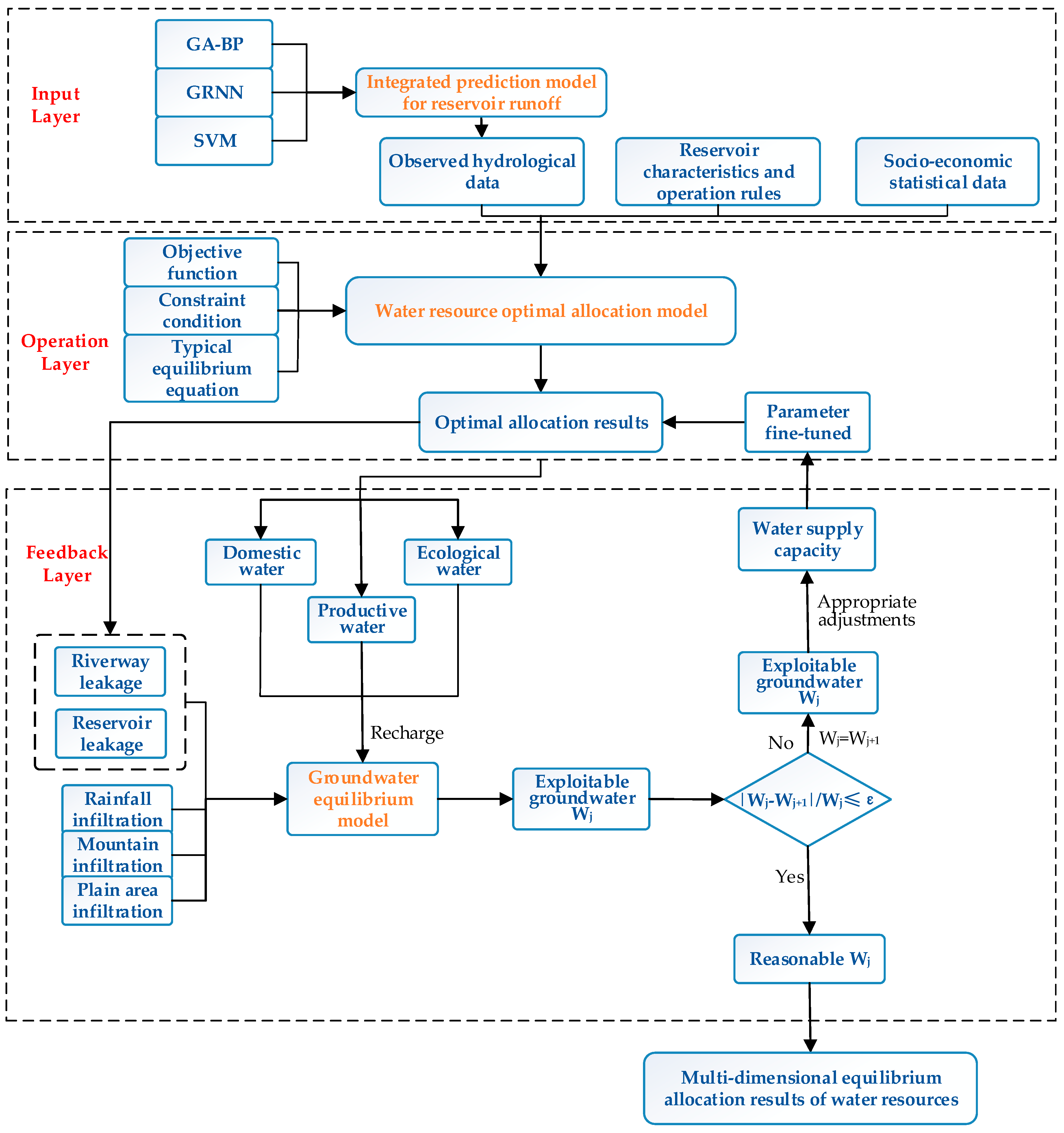
Figure 1. The proposed multi-dimensional equilibrium allocation model of water resources comprises three modules: (a) an integrated prediction module for reservoir runoff; (b) a water resource optimal allocation module; (c) a groundwater equilibrium module. The three modules correspond to the input layer, operation layer and feedback layer, respectively. Furthermore, the layers responds to one another well. It is worth noting that this study focuses on the internal response relationships of these three modules and the integration technology of the multi-dimensional equilibrium allocation model, rather than the single water resource optimal allocation model. Hence, detailed introduction of this module is omitted.
1. Input Layer: The Integrated Prediction Module for Reservoir Runoff.
Factors such as climate, underlying surface condition, and water project construction may affect future allocation plans of water resources. Therefore, it is necessary to predict the quantities of water which will flow into the reservoirs before the optimal allocation of water resources and set the new series of reservoir runoff as the inputs of allocation model.
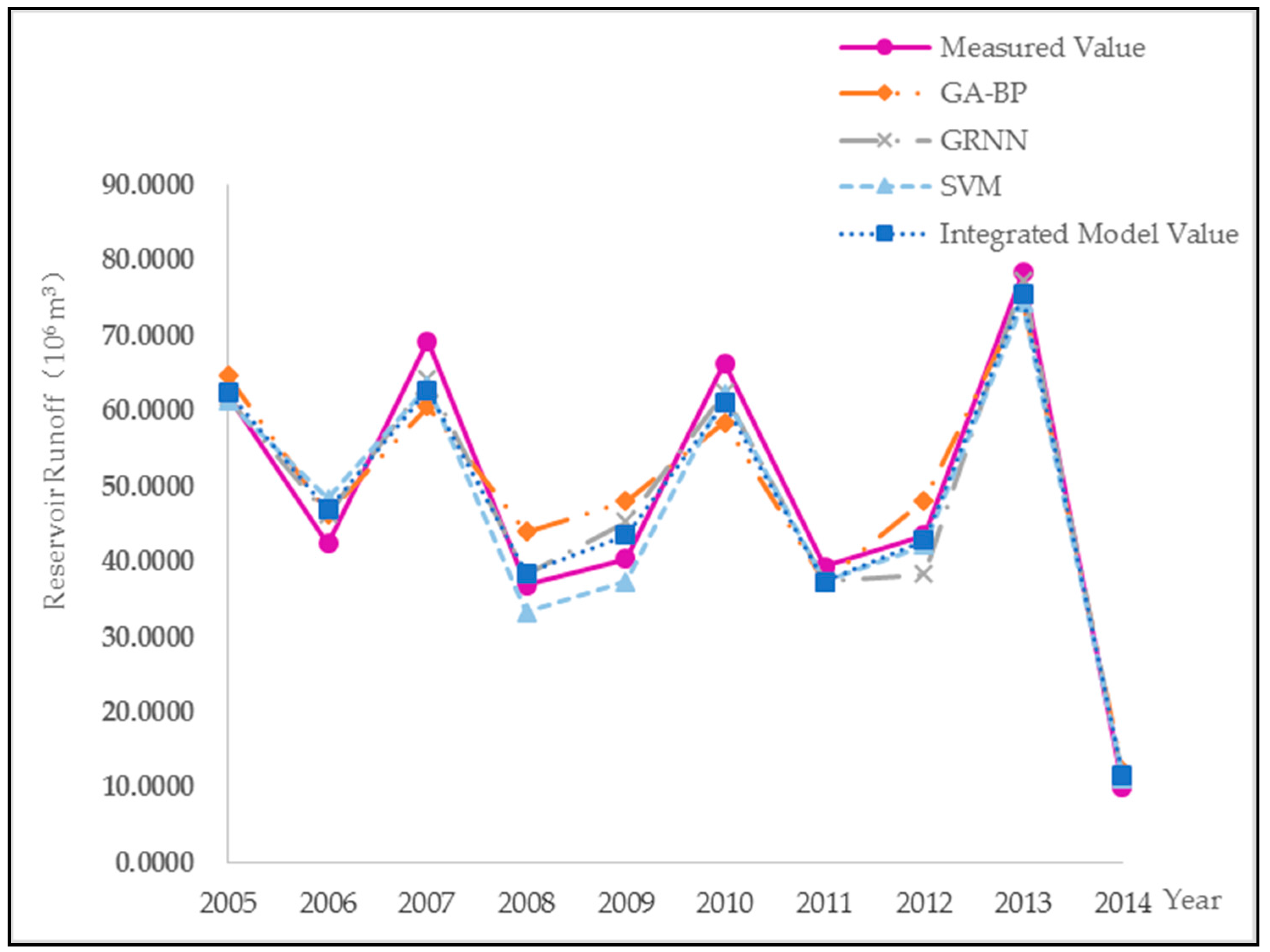
Many single models have been adopted to predict the reservoir runoff in recent years. Nevertheless, the disadvantages of single models under their own operational principles are obvious. Taking the genetic algorithm-back propagation (GA-BP) model [
16] as an example, the ability of the algorithm to adapt the input samples is higher than some other prediction models in previous research, rather, its accuracy is almost the lowest. Hence, the integrated prediction model was employed from three single models to develop their complementary advantages.
The accuracy of prediction model is the most widely accepted indicator which can reflect the difference level between the model prediction value and the measured value. The generalization of prediction model is the most appropriate indicator, which can represent the ability of the algorithm to adapt the input samples. Hence, these two indicators were selected to qualitatively identify the single model weights, and then the integrated prediction model for reservoir runoff was constructed based on the following integration technology [
17,
18].
where
and
are the integrated model prediction value and the single model prediction value, respectively (10
6 m
3).
is the number of single prediction models. In this study, the GA-BP model, general regression neural network (GRNN) model [
19] and the support vector machine (SVM) model [
20] were separately chosen to predict the future reservoir runoff and then
.
is the model weight for each single model and can be calculated based on the following analysis.
The average relative error (
ARE) is selected as the specific indicator to represent the model accuracy. The smaller the
ARE is, the higher model accuracy there is. Meanwhile, the ratio of root-mean-square error (
RMSE) to determination coefficient (
R2) is selected as the generalization (
) of prediction model. The bigger
is, the greater the model generalization is. The specific calculation can be expressed as:
where
and
are the measured value and model prediction value of reservoir runoff (10
6 m
3), respectively.
and
are the average values of measured series and predicted series (10
6 m
3).
is the length of sample series. The single model weights under each indicator can be calculated by the method of normalization expressed as follows.
Weight calculation of the single models under the indicator of accuracy:
Weight calculation of the single models under the indicator of generalization:
Comprehensive weight calculation of the single models:
where
is the comprehensive weight of the
ith single model.
and
are the weights of the ith single model under the indicator of accuracy and generalization.
and
are the weights of the indicator of accuracy and generalization.
2. Operation Layer: The Water Resource Optimal Allocation Module.
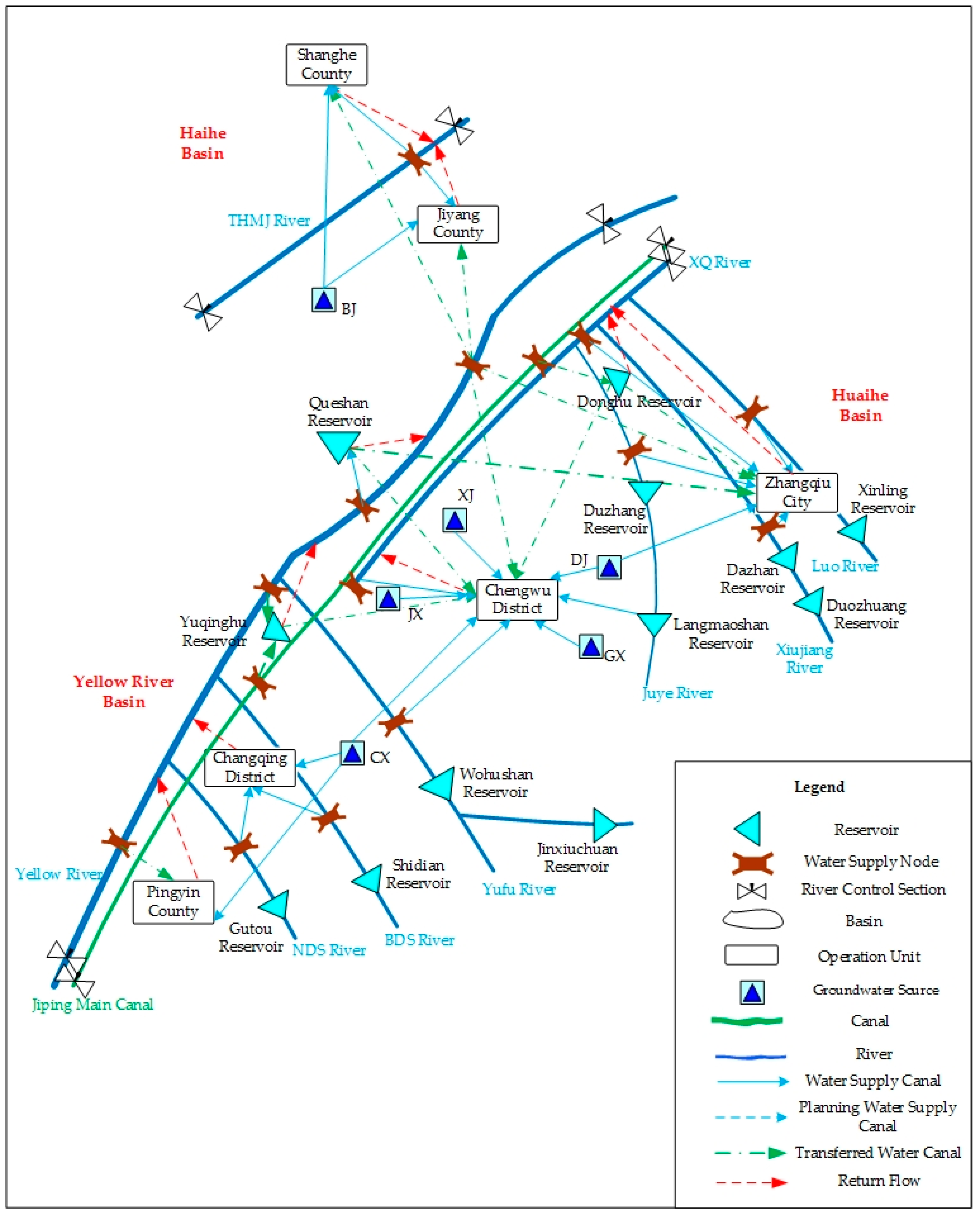
Taking the water resource optimal allocation model as the core [
21], the water resource deployment network chart [
22] is drawn firstly and the first water resource optimal allocation plan is developed based on some relative data, such as the observed hydrological data, reservoir characteristics and operation rules, and socio-economic statistical data, as well as the predetermined optimal rules, constraint conditions, objective functions, and typical equilibrium equations. The purpose of the first optimal allocation is to initially determine the model parameters and simulate the groundwater recharge for the feedback layer.
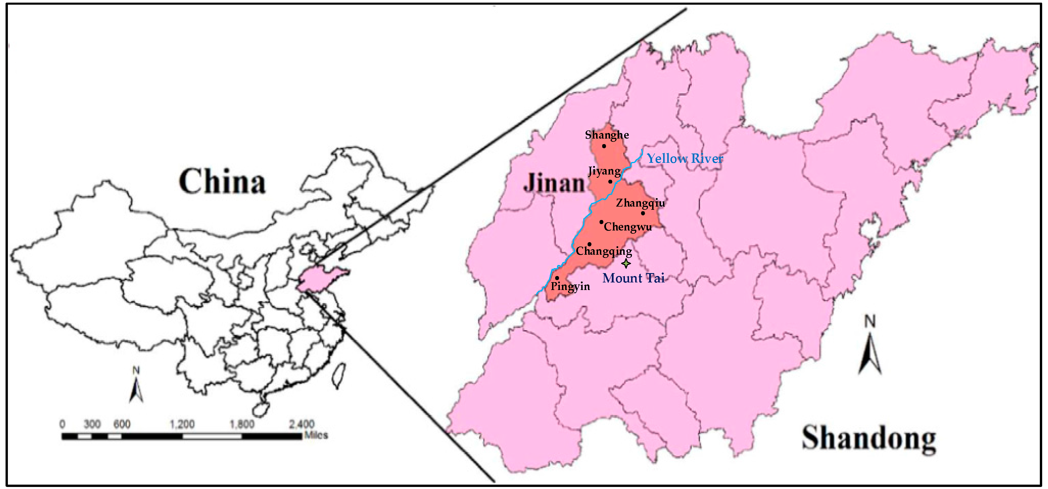
According to the actual situation in Jinan, the water sources in the allocation model should comprise surface water (SW), groundwater (GW), reclaimed water (RW), and transferred water (TW). Three parts form the objective function: (1) the minimum water deficit of society, economy and eco-environment; (2) the maximum water supply benefit; and (3) the minimum reservoir abandonment. The specific computational formulas of the three sub-objective functions, constraint conditions, and typical equilibrium equations can be found in the referenced literature [
23,
24].
where
represents the comprehensive object of the optimal allocation model.
,
and
represent the sub-objective functions of abovementioned three parts, respectively.
,
and
are the weights of the three sub-objects, respectively.
3. Feedback Layer: The Groundwater Equilibrium Module.
The purpose of feedback layer is to modify the water resource optimal allocation results to meet the requirements of multi-dimensional equilibrium. The groundwater equilibrium model was chosen to feedback the exploitable groundwater. The relative results (seen as the groundwater recharge in
Figure 1) from the operation layer should be applied as the input data to the groundwater equilibrium model, such as the recharge amounts of pipe network leakage, riverway and reservoir leakage, and field infiltration and well irrigation regression. The exploitable quantity of groundwater can be calculated according to Formulas (10)–(12), and is then fed back to the operation layer. The groundwater modeling system (GMS) was selected as the groundwater simulation tool and the equilibrium formulas are as follows:
For unconfined groundwater:
For confined groundwater:
where
represents the groundwater recharge which consists of rainfall infiltration, mountain and plain area infiltration, pipe network and riverway leakage, and field infiltration and well irrigation regression (10
4 m
3).
represents the groundwater discharge, which consists of the lateral outflow, spring water discharge, evaporation discharge of phreatic water, and artificial extraction amounts (10
4 m
3).
is the groundwater level variation (m).
and
are the specific yield for unconfined groundwater and the elastic storativity for confined groundwater, respectively.
is the intake area (m
2).
is the time length (s).
The mining coefficient method was adopted as follows:
where
represents the exploitable quantity of groundwater (10
4 m
3).
is the coefficient of allowable withdrawal and it is related to the long-term series data of groundwater, the aquifer type, the mining conditions, and the actual mining status. The calculation of
has been made in our previous research and for Jinan,
in mountain area,
in plain area.
2.2. Multiple-Loop Iteration Technique
The multi-dimensional equilibrium allocation model of water resources proposed in this study is actually driven by the input data and modified by the multiple loop iteration technique of groundwater. Through the monthly calculation and analysis, the water resource optimal allocation plans can meet the requirements of society, economy, and eco-environment, as well as the groundwater balance of exploitation and supplement. The specific operating steps for the multiple loop iteration technique of groundwater can be summarized as follows:
Step 1: According to the regional conditions of water resources, present economic and social situations, and future development planning, the water supply and demand scenarios in different planning periods are set, and the initial optimal allocation model is entered along with the other data. Among which, the integrated prediction results for reservoir runoff are chosen as one of the input data. The initial exploitable quantity of groundwater should be set as , .
Step 2: Through the monthly calculation from the water resource optimal allocation model, the first allocation results for the base year, the short-term (2020), and long-term (2030) periods are obtained initially.
Step 3: Taking the recharge amounts of pipe network leakage, riverway and reservoir leakage, field infiltration and well irrigation regression into the groundwater equilibrium model, the total amount of groundwater recharge can be obtained. Then, the exploitable quantity of groundwater under the first allocation can be calculated according to Formula (12). If (), then proceed to Step 4. Otherwise, set and repeat the previous calculation until it meets the condition.
Step 4: Stop the loop iterative calculation and export the final water resource allocation results. The final results should consist of the water balance between water supply and demand in the base year, the short-term and long-term periods, and the water usage and consumption in all industries, as well as the water supply from all sources.


