Article

Evaluating the Drivers of Seasonal Streamflow in the U.S. Midwest

by
Louise J. Slater
1,* and
Gabriele Villarini
2
1
Department of Geography, Loughborough University, Loughborough LE11 3TU, UK
2
IIHR-Hydroscience & Engineering, The University of Iowa, Iowa City, IA 52242, USA
*
Author to whom correspondence should be addressed.
Water 2017, 9(9), 695; https://doi.org/10.3390/w9090695
Submission received: 3 August 2017 / Revised: 30 August 2017 / Accepted: 8 September 2017 / Published: 12 September 2017

Abstract

:
Streamflows have increased notably across the U.S. Midwest over the past century, fueling a debate on the relative influences of changes in precipitation and land cover on the flow distribution. Here, we propose a simple modeling framework to evaluate the main drivers of streamflow rates. Streamflow records from 290 long-term USGS stream gauges were modeled using five predictors: precipitation, antecedent wetness, temperature, agriculture, and population density. We evaluated which predictor combinations performed best for every site, season and streamflow quantile. The goodness-of-fit of our models is generally high and varies by season (higher in the spring and summer than in the fall and winter), by streamflow quantile (best for high flows in the spring and winter, best for low flows in the fall, and good for all flow quantiles in summer), and by region (better in the southeastern Midwest than in the northwestern Midwest). In terms of predictors, we find that precipitation variability is key for modeling high flows, while antecedent wetness is a crucial secondary driver for low and median flows. Temperature improves model fits considerably in areas and seasons with notable snowmelt or evapotranspiration. Finally, in agricultural and urban basins, harvested acreage and population density are important predictors of changing streamflow, and their influence varies seasonally. Thus, any projected changes in these drivers are likely to have notable effects on future streamflow distributions, with potential implications for basin water management, agriculture, and flood risk management.

1. Introduction

Streamflows—ranging from low to high—have increased notably across the U.S. Midwest (i.e., 12 states of the central USA including Illinois, Indiana, Iowa, Kansas, Michigan, Minnesota, Missouri, Nebraska, North Dakota, Ohio, South Dakota, and Wisconsin) over the past 50–100 years [1,2,3,4,5,6,7,8,9,10]. The consensus is that recent increases in the frequency and magnitude of precipitation events [1,10,11,12,13,14,15] have contributed to these upwards trends in streamflow, particularly since the 1970s. However, streamflow can be altered by a variety of factors, including atmospheric changes (e.g., precipitation type, timing, phase, and volume; temperature; and evapotranspiration), land use and land cover (e.g., urbanization, agricultural practices, ditching and artificial tile drainage), or anthropogenic water management (e.g., dams, impoundment, water abstraction, flow augmentation, and diversions). Understanding the relative influence of each of these drivers on streamflow timing, magnitude, frequency and seasonality is complex, and the aim of attribution studies is to disentangle and quantify the effects of these predictors individually [16].
Over the agricultural Midwest, changes in land use and land cover (LULC) have altered streamflows notably. Deforestation and forest fragmentation have been widespread, with the conversion of grasslands and forests to agricultural row crops of corn and soybean (e.g., [13]) and the expansion of rural and suburban sprawl [17]. The conversion of perennial vegetation to seasonal cropland appears to have amplified the effects of precipitation increases on water yield and baseflow by augmenting groundwater recharge, soil water storage and wetness below the root zone [18,19,20,21]. In Wisconsin, for instance, cropland extension has increased the average annual surface runoff and baseflow [22]. The effects of seasonal crops such as corn and soybean tend to vary for different parts of the streamflow distribution, by increasing the magnitude of high flows during heavy precipitation events and increasing the low flows during dry periods [23]. Many Midwest watersheds, such as the Raccoon River basin, have witnessed increases in corn and soybean land cover from about from one-third to about three-quarters of their entire surface area in the past century [24]. The expansion of artificial drainage across the Midwest reduces water residence time in depressional areas, so water that would previously evapotranspire now reaches the rivers [25]. Alongside these changing drainage and evapotranspiration patterns, increases in CO2 from global warming further reduce plant transpiration, thus potentially increasing streamflows during the growing season [26].
In the urban Midwest, changes in precipitation and temperature have a very different effect on the streamflow distribution. The development of buildings, roads and other infrastructure increases the fraction of impervious land, thereby reducing infiltration and heightening runoff, so floods are larger and peak more rapidly [27,28,29,30]. Recent observed increases in surface runoff and flow in urban Midwest watersheds have partly been attributed to urbanization [22,31,32]. In the Greater Chicago metropolitan area, for example, urban development appears to have heightened streamflow across all flow quantiles (from low to high flows) during all seasons except spring [33]. Sustainable Drainage Systems (SUDS) like detention basins are therefore increasingly required to balance these effects, as part of planning applications. Additional drivers of changing flow distributions in the urban Midwest include the influence of water transfers in and out of catchments (including possible decreased or increased use of groundwater for water supply), water pipe leakage, waste water inflows, and increased summer precipitation arising from High Plains irrigation [4].
Separating these anthropogenic, climatic, and other LULC effects on streamflow is not straightforward, and a variety of modeling methods have been implemented. Attribution is often conducted through case studies [30,34,35] or paired-catchment studies [36,37,38,39]. The latter consists in selecting two catchments with similar physical characteristics, applying a LULC change in one of the catchments, and comparing the resulting reconstituted flows with the observed flows. However, the method has some limitations, as it is time-consuming, difficult to replicate across multiple watersheds, and does not enable the separation of multiple drivers. In contrast, hydrological modeling approaches facilitate the reconstruction of streamflow both with and without simulated disturbances, and can help to estimate the influence of different drivers such as urbanization, regulation, wildfire [40], field drainage [41], or clear-cutting [42].
In contrast, attribution methods using statistical approaches are increasingly being used as time series of observed climate, LULC and streamflow become readily available in many catchments worldwide. Statistical models are easily criticized for lacking the process-based framework of experimental and physical models; yet they tend to be faster to use, allow better definition of model uncertainties, and often produce similar results [43]. Streamflow (Q) can be separated into precipitation (P) and other drivers using various approaches. By aggregating Q and P data over seasonal to annual timescales, any significant shifts in the slope and intercept of the Q-P relationship can be assumed to arise from the influence of other drivers, such as LULC or water management. Conversely, if one assumes a constant Q-P relationship at a given location, then the residuals can be used to investigate the factors characterizing the residual streamflow variability [44]. Simple process-based models based on the Budyko hypothesis [45] may also be used to evaluate the effects of aridity (P and evapotranspiration) and other drivers (e.g., effects of crop conversions, irrigation, reservoir storage and urbanization) [46,47]; or to apportion changes in water yield into climate and LULC drivers [25].
Despite the existence of multiple approaches for disentangling land cover and climatic influences on streamflow, there is still no simple, straightforward method for rapidly assessing which of these drivers play a dominant role in any given region. Building on previous work, which shows that streamflow can effectively be modeled using precipitation and land cover as covariates [24,31,32], we hypothesize that simple statistical models can be used to identify the most important predictors (drivers) for modeling streamflow in a given region. We then use generalized additive models (i.e., where the predictor depends linearly on smooth functions of the predictor variables), to model the streamflow time series under non-stationary conditions, using agriculture, population, precipitation and temperature as potential predictors. Our research questions are as follows: how well can statistical models describe year-to-year variations in seasonal streamflow quantiles? Is there a regional distribution to the types of predictors that best fit the data (for example, can simple predictors such as basin-averaged temperature or population density be used to improve model fits in snowmelt-dominated or urban basins)? How might future changes in these predictors affect streamflow distributions? We conduct the analyses at the seasonal scale to facilitate the detection of potential flow-generating mechanisms. Overall, our approach can be considered as a novel methodology for “soft” attribution [16], enabling the identification of relevant regional and seasonal streamflow drivers within a systematic statistical modeling framework.

2. Materials and Methods

2.1. Data

For the analysis, we selected all U.S. Geological Survey (USGS) stream gauges in the 12 Midwest states (North Dakota, South Dakota, Minnesota, Nebraska, Kansas, Iowa, Missouri, Wisconsin, Illinois, Michigan, Indiana, and Ohio; Figure 1) that were still active (i.e., recording streamflow) in 2015. We downloaded all the mean daily streamflow data for these sites from the USGS NWIS website [48].
Within the observed streamflow time series, we retained only complete water years (at least 330 days, i.e., 90% of mean daily streamflow measurements) and required a continuous record of at least 50 years. We used a conservative approach, allowing no gaps in the data (even though small gaps are not prohibitive for time series analysis [49]). To ensure that statistical models were fit only in sites without major anthropogenic influences, we removed any sites where flags 5 or 6 (discharge affected to known or unknown degree by regulation or diversion) were present in the USGS’ peak flows database [48]. Our aims are not to quantify climatic or anthropogenic impacts on streamflow variability specifically, but to assess the main drivers of changing streamflows across the entire study region. For information on model fits at any specific site (e.g., in a regulated basin), we recommend consulting the Supplementary Materials, where all time-series data and model fits are provided.
The streamflow time series at each site were split into seasons, retaining only complete (i.e., with three months) seasons: winter (December–January–February (DJF)), spring (March–April–May (MAM)), summer (June–July–August (JJA)), and fall (September–October–November (SON)). Streamflow quantiles were computed from Q0 (minimum daily flow) to Q1 (maximum daily flow) with a step of 0.05 (a total of 21 quantiles), for every season. The drainage basins of our 290 sites range from 20 km2 to 153,327 km2 in size; time series length ranges from 50 to 76 continuous years.
To model the seasonal streamflow quantiles from low to high flows, we use precipitation, temperature, population data and agricultural land coverage as predictors (Table 1). All the predictors are basin-averaged values. Time series of streamflow and basin-averaged predictors are shown for every one of the 290 sites in Figure S1 (Supplementary Materials).
The first two predictors, precipitation ( x p ) and temperature ( x t ), were computed using data from the PRISM climate group [50], which are freely available online from 1890 to the present. PRISM’s temporal and spatial resolutions are monthly and approximately 4 km. PRISM climate data prior to 1950 may be less suitable for trend analyses than later data, due to the sparseness of meteorological stations in the 1902–1950 period [51,52]. However, our analysis only extends as far back as 1940 (when those data are available), so we consider that this is not a major issue. At every site, we first compute monthly time series of the mean monthly basin-averaged precipitation (or temperature), using the basin boundaries from the USGS Streamgage NHDPlus Version 1 [53]. We aggregate the total seasonal precipitation as the sum of three mean monthly values (in mm), and the seasonal temperature as the mean of the monthly values (in Kelvin degrees, so the scale is similar to that of precipitation). We include two additional seasonal temperature predictors in our Mixed model: the mean temperature at the start of spring, to reflect the influence of temperature on snowmelt (March–April temperature, x t m a r a p r ) and the mean temperature at the start of summer to reflect evapotranspiration (June–August temperature, x t s u m m e r ) (see Section 2.2. for model formulation).
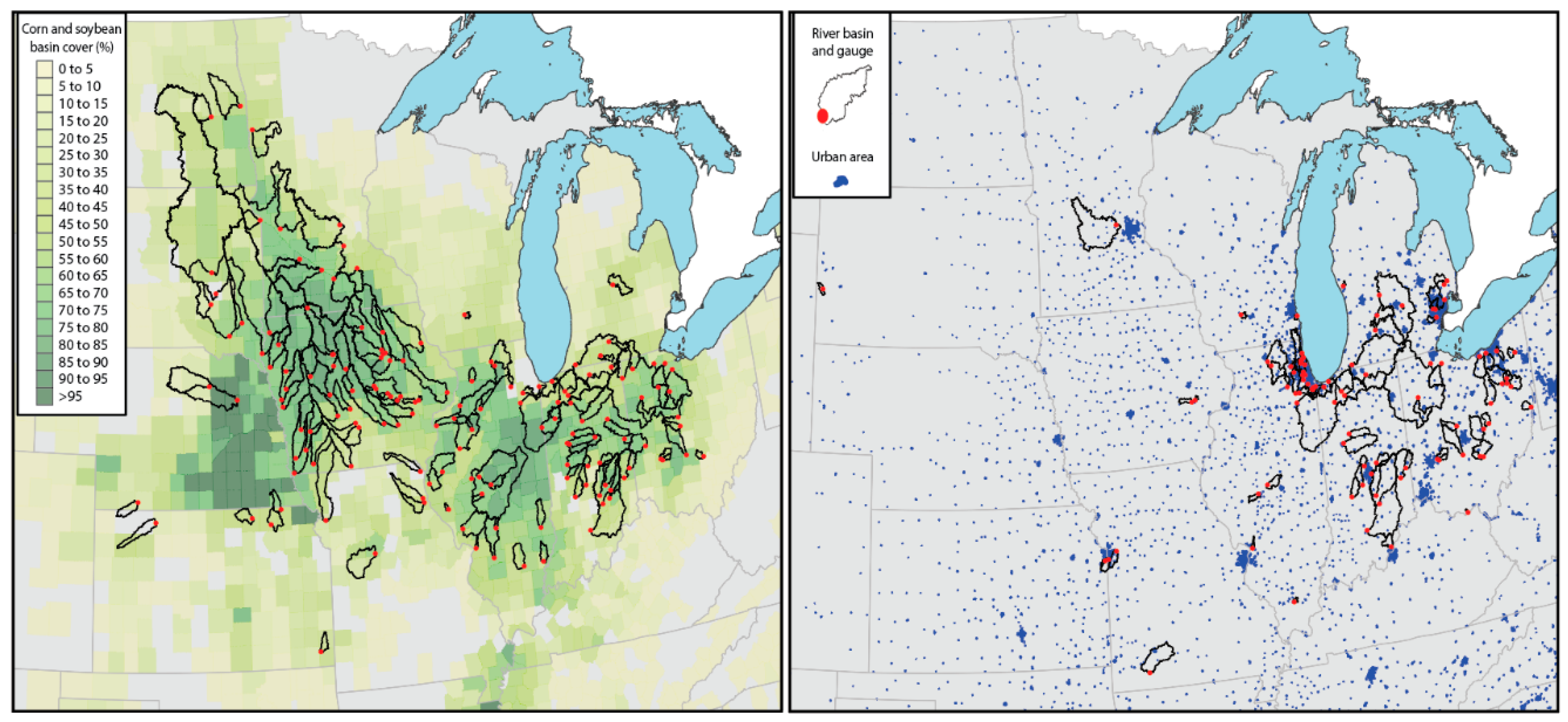
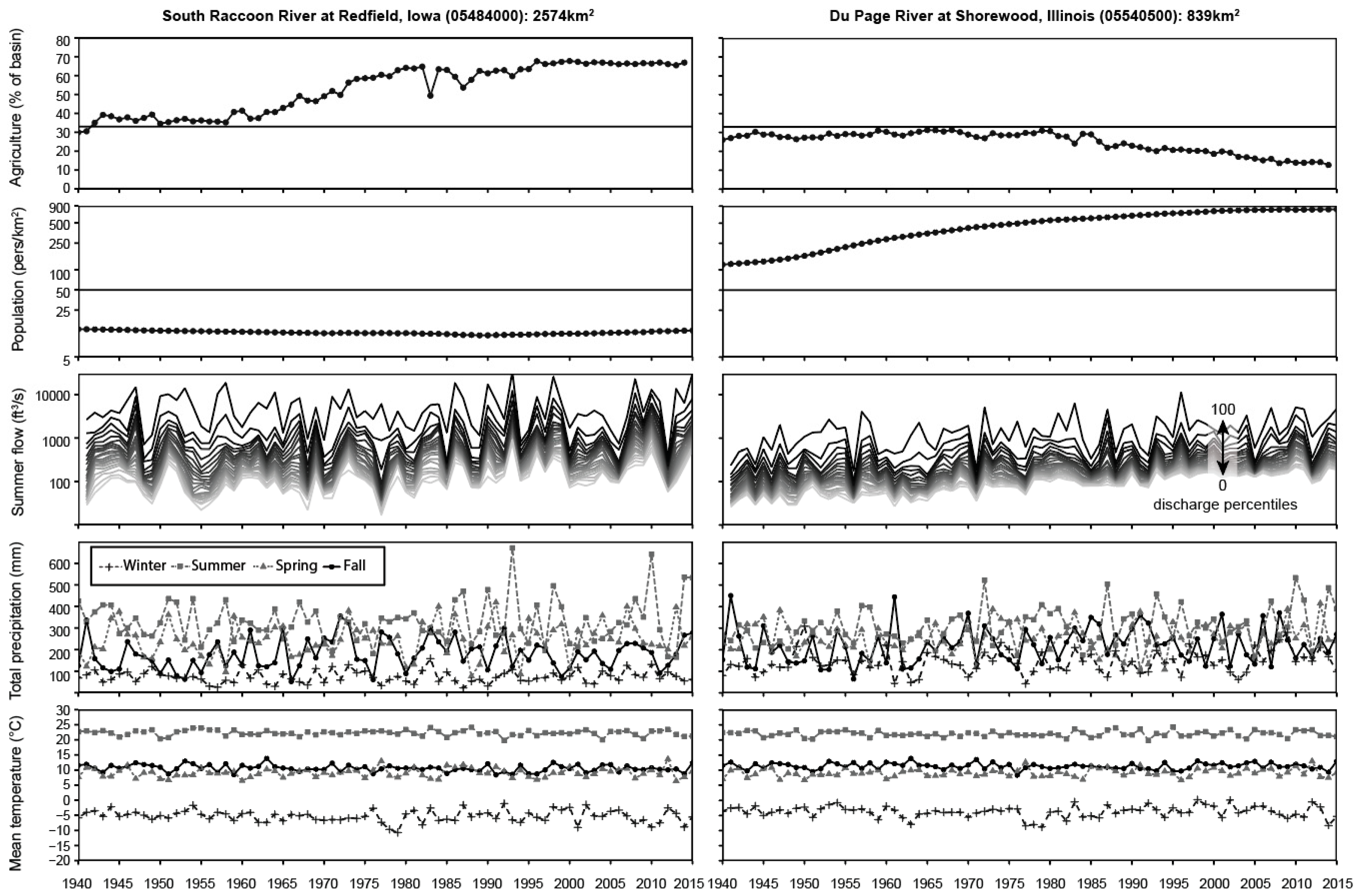
To represent the effects of agricultural practices (predictor x a ) on the flow frequency distribution, we use the harvested acreage of combined corn and soybean, i.e., the two most widespread crops the Midwest in terms of percent of harvested cropland acreage [54], following [18,23,24]. In many agricultural basins across the Midwest, there has been a progressive increase in agricultural land cover during the 1940s–1990s (e.g., [18,19,23]). County-level data are obtained from the U.S. Department of Agriculture’s National Agricultural Statistics Services (NASS) quickstats database at USDA.gov [55]. Total harvested acreage is computed as the total of annual values of corn and soybean acreage (the latter are also often in rotation with corn). For every site, we calculate the basin-averaged harvested acreage by first computing the fraction of each county that lies within the limits of the watershed, and, assuming that the crops are distributed evenly across each county, multiplying each fraction by the total agricultural acreage of that county. The total acreage within each watershed is then calculated as the sum of all values across all counties. This process is repeated every year to obtain a time series of total annual cultivated corn and soybean acreage as a percentage of each watershed, for every site. For the last year of the dataset (2015), agricultural data were not yet available at the time these analyses were performed, so we used the data from 2014, assuming that there would be little change in cropland from year to year (e.g., [23]). We use annual values in the models (Table 1) as there is no seasonal variation in the existing available data. We considered watersheds as agricultural if the harvested acreage covered at least 33% of the watershed at any given point in the historical time series (Figure 2, left); we used x a as a predictor only in these basins. For an example of an agricultural site, see the South Raccoon River at Redfield (Figure 3, left), where the proportion of agricultural land cover (corn and soybean) has increased from 30% in 1940 to 67% in 2014.
To represent the influence of population density on streamflow, we used demographic statistics as a predictor ( x p o p ). We assume that changes in catchment population will affect streamflow extractions and wastewater returns. In rapidly urbanizing catchments, increased development and impervious land may also modify runoff patterns [27,28,29,30]. Because there is no existing dataset of county population estimates at the annual timescale, we compiled county population data from 1900 to 2015 from three sources: (i) decadal data from 1900 to 1970 from the Decennial census data [56]; (ii) annual intercensal data from 1970 to 2014 from the National Bureau of Economic Research (computed from the Census Bureau’s Population Estimates Program) [57]; and (iii) 2015 values from the U.S. Census Bureau’s Population Estimates Program [58]. We assembled the time series and computed any missing years (particularly during 1900–1970, where we only have decadal data) by fitting a Locally weighted scatterplot smoothing (Loess) curve [59] to the time series with a relatively flexible span of 0.09 (the span was selected empirically by observing the data and choosing the most plausible fit) and interpolating the missing values. Once complete annual county-level time series were assembled, we computed the time series of annual basin-averaged population per square kilometer in the same manner as for the agricultural data. We considered any basin with more than 50 persons/km2 at any given point in the time series as urban (Figure 2, right). This threshold is lower than that of 150 persons/km2 selected by Hirsch and Ryberg [60] because our catchment-averaged value of 50 persons/km2 can include some more localized, densely urbanized areas. An example of a progressively urbanizing site is shown in Figure 3 (right): the population density in the Du Page River basin has increased from 120 persons/km2 in 1940 to 803 persons/km2 in 2014.
Finally, “basin wetness” (predictor x m ) was computed using the precipitation data (described above) from the three months preceding each season as a proxy for antecedent wetness. For example, for the summer season (JJA), we use the total precipitation (in mm) from March–April–May. We recognize that wetness could be characterized by shorter or longer timescales (from months to years) depending on the catchment morphometry [10] but have chosen three months as a reasonable estimate for modeling seasonal streamflow distributions.
Other drivers could have been considered (e.g., potential evaporation), as well as interactions (e.g., potential evaporation and precipitation). However, as a first approach, we decided to keep a relatively small number of main drivers, in locations where they were deemed physically reasonable (hence our decision to use predictors x p o p and x a only in urban and agricultural basins, respectively). The original list of sites was tailored to retain only the 290 sites that had streamflow, precipitation, temperature, agriculture, and population data. At each site, the predictor time series were cropped to begin in the earliest year in which all of the variables (streamflow, precipitation, temperature, population/agriculture if relevant) were available.

2.2. Model Formulation and Selection

We fit seven statistical models to the observed seasonal streamflow quantiles, using basin averaged precipitation ( x p ), basin-averaged temperature ( x t ), basin percentage of agricultural row crop acreage ( x a ), basin-averaged population density ( x p o p ), and antecedent precipitation (a proxy for antecedent wetness; x m ) as predictors, following a similar methodology to [23,24,61] (Table 1). These predictors are evaluated in different combinations to assess which model formulations can best characterize the flow distribution. It is likely that at any given site there will be multiple drivers of change, and the relative influence of each driver may vary depending on the chosen timescales [41] and seasons. We restrict the analysis to consider just those seven models rather than all possible combinations, which would have been too numerous.
To develop the models, we use Generalized Additive Models for Location, Scale and Shape (GAMLSS [62]) for statistical modeling of time series, using the gamlss package in the open-source software R [62]. We chose the gamma distribution because it was found to be a good candidate distribution for modeling streamflow (with well-distributed model residuals) in previous studies [23,24]. In all of the models, μ and σ are the two parameters of the gamma distribution (Table 1). Based on the parameterization in GAMLSS, the expected value of Y is equal to μ and the variance to σ2μ2. The σ parameter is held constant because previous work indicated that it was not significantly dependent on precipitation and agriculture [23]. The predictand Y represents a quantile of the seasonal streamflow time series ranging from minimum (Q0) to maximum (Q1) flow. For instance, if Y represents the spring Q0.5, we would compute the median of the daily flow distribution for the three-month period ranging from March to May (MAM), annually, from every spring Q0.5 with complete data. For convenience, we refer to the seven models as P, P.T, P.M, P.PA, P.Ppop, P.PA.M, and Mixed henceforth; the predictors are listed in Table 1 and each model is described fully below.
Model P describes streamflow variability solely as a function of changing precipitation (predictor x p ). Model P.T describes streamflow as a function of precipitation and temperature (predictor x t ). Model P.M incorporates the effects of antecedent wetness (predictor x m ) on streamflow.
Models P.PA, P.Ppop and P.PA.M consider how precipitation varies with different interaction terms that may affect the flow distribution. Thus, instead of using the predictors for population density, agricultural land cover, and antecedent wetness as separate terms in the equations, the predictors are multiplied by precipitation and considered to act as a runoff coefficient that strengthens or weakens the streamflow-precipitation relationship. In other terms, both agriculture (corn and soybean land cover) and population densities (via increasing extent of impervious land cover) are expected to alter the P-Q relationship via their effect on spatial runoff patterns and intensities. Model P.PA considers the interaction between x p and changing agricultural land (predictor x a ), measured as a percentage cover of the basin; model P.Ppop considers the interaction between x p and changing population density (predictor x p o p ). The sixth model, P.PA.M, considers the interaction between x p and agricultural land cover, as in the P.PA model, but also includes the influence of antecedent wetness (predictor x m ).
Finally, the Mixed model includes both antecedent wetness (as in model P.PA.M) and temperature. The model formulation varies seasonally to reflect different temperature drivers in different seasons. In the spring, it includes the mean temperature from the beginning of the season (predictor x t m a r a p r ) to reflect the influence of temperature on snowmelt. In the summer and fall months, the Mixed model includes the mean summer temperature (predictor x t s u m m e r ), to reflect evapotranspiration in the summer and antecedent basin wetness in the fall.
To evaluate which of these models performs best at each gauging station, we use the Akaike Information Criterion (AIC; [63]), which reflects the trade-off between parsimony and goodness-of-fit. The approach is similar to the one used in [64], where the best fit GAMLSS model is chosen in terms of the predictors and their functional relation to the parameters of the probability distribution. For each model, we also perform leave-one-out cross-validation: for every year, we remove the given observed value, and predict it with the rest of the observations, repeating this process every year until we have a complete time series. We then assess the cross-validation results by computing the correlation coefficient R between that time series and the observed data. The goodness-of-fit of models P.PA and P.PA.M is described in some detail in [24] in terms of the mean, variance, coefficient of skewness, coefficient of kurtosis, and Filliben correlation coefficient of each of the streamflow quantile residuals.

3. Results and Discussion

3.1. Model Fits

At all 290 sites, for every season and every quantile (ranging from Q0 to Q1, with a step of 0.05), we fit the models described in Table 1 (see Figure S2). We illustrate the fits here using model P.PA for the South Raccoon River at Redfield (an agricultural basin) and model P.Ppop for the Du Page River (an urban basin), for low, median and high flows (Q0.05, Q0.5 and Q0.95) (Figure 4). Our seasonal model fits are probabilistic and thus are displayed as a probability distribution for every year. In other words, instead of fitting a single value, we are fitting a full probability distribution: percentiles 5, 25, 50, 75 and 95 are shown for every year using color ribbons in Figure 4.
Using the AIC as our metric, we assess which of the seven models produces the best fit to the observed flow time series at every one of the 290 sites (note that not necessarily all seven models are fitted at every site, since the agricultural predictor is only used in agricultural catchments, and the population density predictor in urban catchments (see Section 2 for details); sites can have neither predictors or both). The results of the best model selection are summarized across all flow quantiles in the color map (Figure 5). Time-series graphs are provided for the best-fitting models for Q0.05, Q0.5, Q0.95 and Q1 for every site and season in Figure S2 (similar to the time series graphs shown in Figure 4). Additionally, we provide a spatial summary (maps) of the best-fitting seasonal models for every one of the 21 quantiles in Figure S3.
We expect to find regional differences in model fits depending on precipitation seasonality, climatic differences, and the prevalence of urban or agricultural land (Figure 6). Across the study domain, precipitation increases from northwestern Minnesota (~500 mm or 20 in) to southern Missouri (1175 mm or 47 in) [12]. The largest (annual maximum) daily precipitation events occur mostly during the summer months [15]. While the frequency of precipitation events is greatest in the summer, it is also relatively high in the spring (especially over the western half of the region—South Dakota and Nebraska), and is concentrated in the Northeast (Michigan) and South (Missouri) of the study domain in the fall [15]. Corn and soybean crops are typically planted from April to June (with the southernmost regions planting first, and the northernmost planting when soils thaw); and the harvest is in late September/October to November. Additional differences in model selection are likely to be related to factors such as catchment size and land cover types. Catchment size varies considerably across the 290 basins and is likely to affect the main runoff processes at each site (here we focus mainly on the existence of broad regional predictors characterizing the flow distributions).
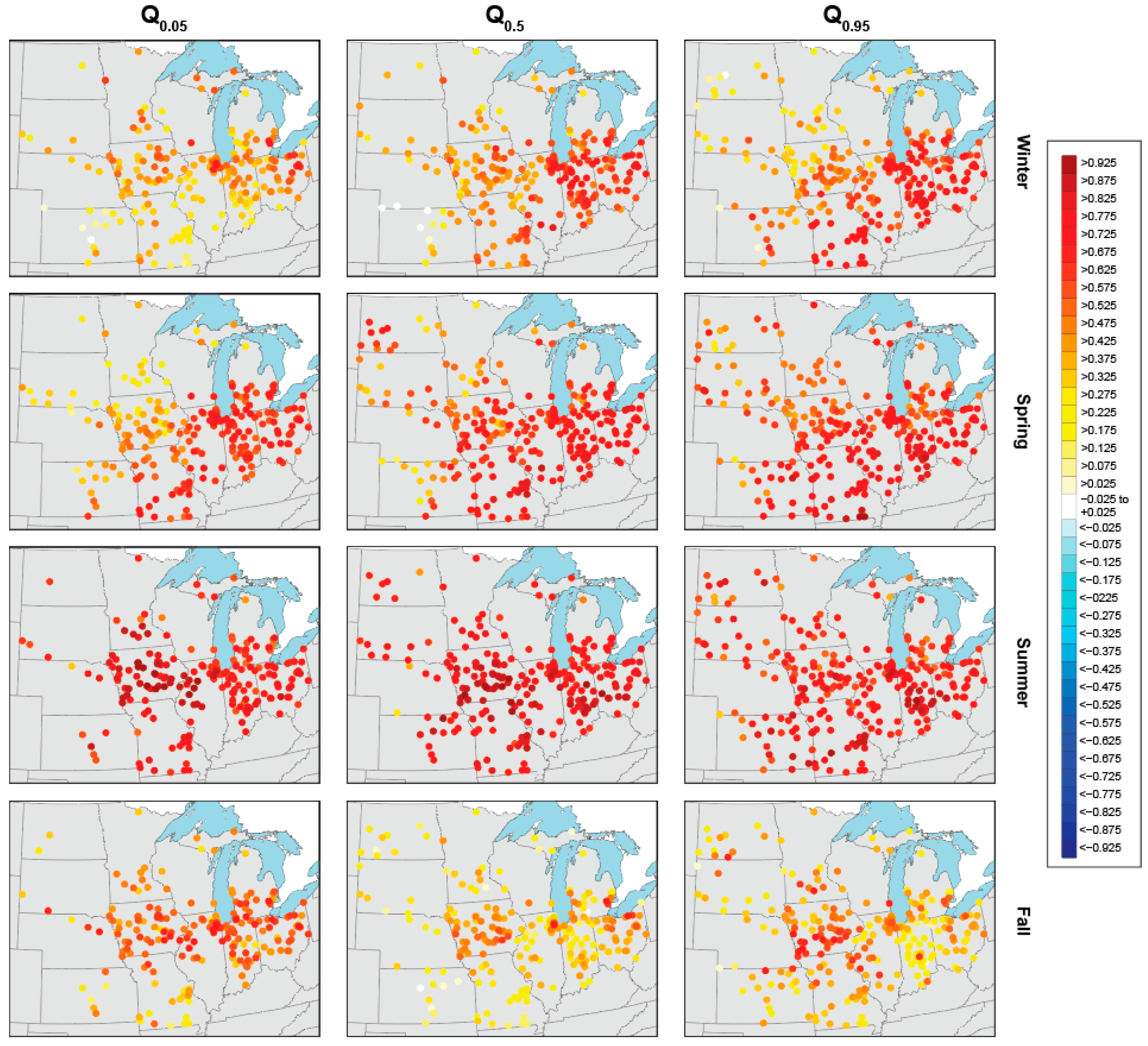
Overall, the streamflow distributions are best fit during the wetter months (average R = 0.64 for spring, R = 0.77 for summer) and less well-fit during the cold and drier months (average R = 0.40 for fall, R = 0.51 for winter) across all 20,996 model fits (all sites, models, and flow quantiles; see Figure 7 for the correlation coefficients at a subset of quantiles and Figure S4 for all quantiles). When comparing the fits for different flow quantiles, we find that there is not much difference: the high flows (Q0.7Q0.95: R ≈ 0.6) are only slightly better modeled than the low flows (Q0Q0.1: R ≤ 0.57).
Spatially, the best model fits are found in the southern Midwest (R often > 0.7, except in fall), where flooding tends to occur in early spring and displays a strong seasonality [65]. Model fits are slightly less accurate in the northwest of the study area (i.e., Minnesota, the Dakotas, Nebraska and Kansas; R < 0.3), where flooding tends to occur later in the year and seasonality is less well-defined [65].
To evaluate how well our models perform, leave-one-out cross-validation was carried out for the best-fitting model at every site (Figure 8). Overall, the correlation coefficients for cross-validation are high, indicating that model skill is particularly good in the areas where the models fit well (southeastern part of the study domain). In the other regions (northwestern and southwestern areas especially), some negative correlation coefficients can be seen.

3.2. Precipitation

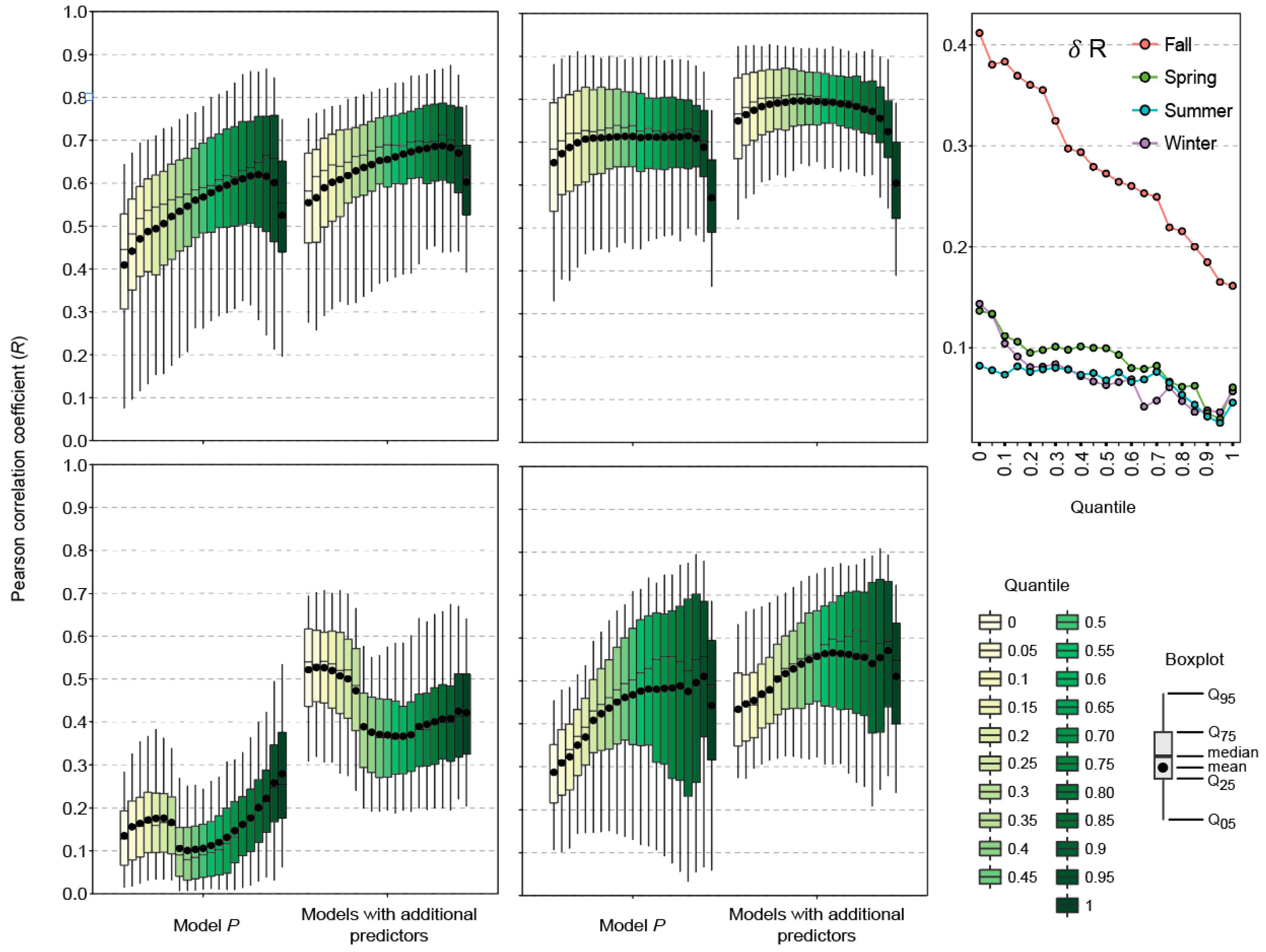
Across all seasons and all flow quantiles, we compare the relative importance of each predictor to precipitation (predictor x p ). Across the 18,815 model fits (for all seasons, sites, and flow quantiles) where model P is not the best fit, the average correlation coefficient is R = 0.48 for just model P, and increases to R = 0.60 when using the best model (smallest AIC) instead, i.e., when additional predictors are included (Figure 9). In other words, the x p predictor clearly explains most of the variability in the data, and the other predictors act as vital interaction terms that strengthen or weaken the Q-P relationship.
The enhancement of model skill that comes from including additional predictors is the most marked in the lower quantiles of the streamflow distribution (average increases in R of ~+0.15 for quantiles Q0 to Q0.5) and the least in the upper quantiles (average increases of +0.11 for Q0.55Q1; Figure 9). Likewise, the increases in model skill are the strongest in the fall months (+0.24), which have the poorest model P fits, and the weakest in the summer (+0.09) which have the strongest model P fits. These findings suggest that the inclusion of additional climatic and LULC predictors is most beneficial in the lower flow quantiles where antecedent wetness and groundwater levels play an important role in modulating the precipitation-streamflow relationship. Model P (i.e., where x p is the only predictor) is rarely the best-fitting model, except for spring maximum flows in the southeastern Midwest (Figure 5, Figure 6 and Figure S3).

3.3. Antecedent Wetness

Antecedent wetness is our second most important predictor: 61% of all of the best-fitting models (i.e., 20,996, across all 21 flow quantiles, seasons and sites) include x m , mostly in the spring, summer and fall. In the spring, the low flows (Q0Q0.25) are best characterized by P.PA.M, and the rest of the flow distribution by the Mixed model (Q0.30Q1; Figure 5, Figure 6 and Figure S3). In summer, the most common best-fitting models are Mixed for low and median flows (Q0Q0.55) and P.M for high flows (Q0.8Q1; Figure 5, Figure 6 and Figure S3).
In the fall, the influence of antecedent wetness is particularly marked. P.PA.M is consistently the most common best-fitting model for low-median flows (Q0Q0.7) and P.M for high flows (Q0.75Q1). In fact, the considerable jump in the model skill shown in Figure 9 for the low flows (Q0Q0.3) is largely due to the improved characterization of soil moisture in the models: 77% of the fall model fits where R increased by more than 0.3 included the x m predictor. These findings suggest that the antecedent wetness of the basin is the most important driver for low and median flows (Figure 5, Figure 6 and Figure S3). It is well-established that antecedent wetness plays a major role in controlling the flow distribution [66,67,68]. In fall, it appears that the wetness from previous months ( x m ) interacts with any agricultural land cover ( x a ) and conditions the flow distribution. The control of P.M. on high flows is also in agreement with previous findings suggesting that the long-term antecedent rainfall controls flood peaks across the Midwest [10].

3.4. Agriculture

The overall influence of agricultural land cover and of changing agricultural practices on streamflows across the Midwest has led to heated debates in recent years [20,69,70,71,72,73,74,75,76]. In the Upper Mississippi River Basin, LULC has a clear signature on streamflow [77]. Previous work attempting to disentangle the effects of climate change, cropland expansion and artificial field drainage (using a hydrologic model) showed that increased precipitation and reduced evaporative demand were a stronger driver of increasing flow than the LULC changes [13]. In contrast, two studies in Iowa considered the relative effects of changing rainfall and harvested corn and soybean acreage on streamflow, and found that projected streamflow increases could be mitigated by decreasing agricultural production [78,79]. We do not seek to settle the debate or to determine the exact influence of agricultural land cover (or of artificial drainage) on changing streamflows, as this would require a finer resolution than the seasonal time scales considered here. However, our approach does suggest that changes in harvested acreage are reflected in seasonal streamflow distributions across the 290 sites. In the 154 agricultural sites (i.e., in catchments with more than 33% of agricultural land cover, where x a was included as a predictor), models P.PA and P.PA.M were selected as the best-fitting model 50% of the time (among all seven models and across all seasons and quantiles). These two models are most important for the low and median flows: in spring and fall, P.PA.M. is the most common model for characterizing low and median flows, while in winter, P.PA best characterizes the low flows (see Figure 5, Figure 6 and Figure S3.) This prevalence of x a in the best-fitting models for low flows suggests that shifts in the fraction of cultivated agricultural land do have a notable influence on low flows. Overall, it is likely that the influence of agriculture on streamflow distributions will also depend on the type of crop and complex interactions among different LULCs [77] and climate.

3.5. Temperature

In spring and summer, the inclusion of seasonal temperature (predictor x t ) within the Mixed model often produces a better fit than using just x p and x m as predictors (compare the number of times the Mixed model was selected in comparison with P.M. and P.PA.M in Figure 5). Thirty-two percent of all the best fits (across all flow quantiles, seasons and sites) include x t as a predictor. This improvement of model fit through the inclusion of temperature is to be expected, as runoff and antecedent soil moisture storage are controlled by the combined influences of rainfall and evaporation [68]; around 60% of global terrestrial precipitation is evaporated [80], with most evaporation occurring in the warmer months of the year.
In the U.S. Midwest, there have been notable changes in temperature over the last century. In South Dakota, for example, warming temperatures have led to earlier spring snowmelt, with higher flows in winter and spring [81]. Here, the spring median and high flows (Q0.5 to Q1) are best characterized by the Mixed model (see Figure 5), suggesting that the temperature at the start of the season (predictor x t m a r a p r ) is an important control on spring flows, likely through the influence of snowmelt. In the winter, Model P.T is the best-fitting model for the median and high flows (34% of sites for Q0.5 and 44% for Q1; Figure 5); see, for example, in Michigan and northern Indiana (red circles in Figure 6 and Figure S3). In many of the smaller catchments, streamflow is likely to freeze during the winter months. Thus, potential applications of this modeling framework include understanding the influence of predictors like temperature on the direction of change (increases/decreases) in streamflow. In Idaho, for instance, rising temperatures appear to have led to increasing flows in the winter, but decreases in the spring and summer [82].

3.6. Population Density

The P.Ppop model (black circles in Figure 6 and Figure S3) is rarely one of the dominant models, but this is partly because we restricted the use of x p o p as a predictor to the sites with a population density of more than 50 persons/km2. While P.Ppop is only the best-fitting model 11% of the time (when considering all sites, seasons, and flow quantiles), it is nonetheless the best-fitting model 32% of the time in the 91 urban basins where the model was fit. Further, if we focus on the most densely-populated basins (Figure 2, right panel; especially around the urban areas of Chicago, Detroit, Cleveland, Columbus and Indianapolis), the P.Ppop model is frequently one of the best-fitting models, especially in the winter and fall (Figure 6 and Figure S3).
Existing work on the effects of urbanization in the Midwest has mostly focused on individual watersheds, but there is increasing evidence to suggest that population density can have a dramatic effect on flood hazards. In the Milwaukee metropolitan region, marked hydrologic variations were found in response to localized increases in flood peak magnitudes and flood frequency, with higher rainfall rates and larger flood peak discharges in the studied urban catchment, in comparison with an adjacent agricultural catchment [83]. In the Chicago area, the spatial distribution of rainfall and the degree of urbanization control the magnitude of the runoff response, so the flood peak distribution has evolved in response to the progressive urbanization [32]. Here, our results also suggest that population density is a much-overlooked predictor of flood response (Figure 10).
Figure 10 illustrates the effects of changes in the key drivers briefly by conducting a meta-analysis across all of the 290 sites (using the best-fitting model for each flow quantile and season at every site) and considering the effects of a change of +10%, +5%, −5% and −10% in three of the predictors ( x p , x p o p , and x a ). For each of the corresponding models, P, P.Ppop and P.PA, we vary (i.e., increase or decrease) only the predictor of interest. For example, in the P.Ppop model, the x p time series remain the same, and only the x p o p predictor changes. We focus specifically on the spring and summer months for the sake of flood design, because high flows in the Midwest are more likely to occur during these two seasons [7,65], and because those were the seasons where we achieved the best model fits.
Results indicate that the influence of precipitation, population density and agriculture on the flow distribution is surprisingly similar in terms of magnitude (even though we did not expect that changes in these driving factors would have similar rates). In fact, the magnitude of changes in streamflow appears to be more sensitive to the season and flow quantile that is being considered than to the choice of predictor. Increases in these three predictors of +10% may increase streamflows by up to or more than 30%, depending on the flow quantile. High flows are more sensitive to increases in precipitation than low flows, particularly in the summer, as has been found previously [84].
In contrast, if we consider x p o p and x a in spring, the low flows appear to be more sensitive to increases in the predictors than the high flows. Perhaps the most surprising effect here is that during the summer, an increase in population density of 10% may increase the median streamflow by >20%. Others have also shown that the effects of population density can be greater than that of other LULC changes like deforestation [22]. Similarly, decreases in the three predictors of 10% also have comparable effects in terms of their influence on streamflow magnitude. Decreases in precipitation are the most influential for the upper quantiles of the flow distribution. This is also true for population density ( x p o p ) in the summer months. In the spring, however, decreases in the predictors x p o p and x a have a stronger effect on the lower quantiles of the flow distribution. Overall, the framework proposed herein points to one main conclusion: when considering dominant regional drivers over seasonal timescales, LULC and population density are just as important as climate.

4. Conclusions and Future Directions

This paper describes a “soft” attribution experiment to systematically evaluate the key drivers of seasonal streamflow in the U.S. Midwest. Time series of basin-averaged precipitation, temperature, population, and harvested acreage (including proxies for antecedent wetness, snowmelt and evaporation) were computed in 290 river catchments with active USGS stream gauges. For every site, season, and streamflow quantile, we fit seven GAMLSS statistical models using different combinations of the predictors, to assess which model formulations best characterized the flow distribution. The performance of these models was assessed using the AIC as our evaluation metric, alongside leave-one-out cross-validation. Our results illustrate that a systematic statistical modeling framework can indeed be used to identify the most important predictors for modeling streamflow in a given region and season.
Overall, the models describe interannual fluctuations in seasonal streamflow quantiles remarkably well, with clear spatial differences in the types of predictors that best characterize the data for different seasons. The model fits are slightly better during the warm and wet seasons (average R = 0.7 in the spring and summer) than during the cold and dry seasons (R = 0.46 in the fall and winter). High flows tend to be slightly better modeled than the low flows, and the best model fits are found in the southern part of the domain, with a decrease in skill towards the drier Northwest.
When comparing drivers, we find that model P (i.e., where precipitation, x p , is the only predictor) is rarely the best-fitting model, except in the winter over the southern part of the study domain. Antecedent wetness (predictor x m ) is our second most important predictor (included in 61% of all of the best model fits across all flow quantiles and seasons), and is a strong predictor for low and median flows (models P.M and P.PA.M). In the spring and summer, the inclusion of temperature (predictor x t ) in the Mixed model often produces a better fit than using just x p and x m as predictors. In spring, the inclusion of temperature at the start of the season (predictor x t m a r a p r ) improves model fits for medium and high flows, likely through its effect on snowmelt. In winter, P.T is the best-fitting model for median and high flows, and suggests that cooling temperatures also alter the flow distribution. Harvested acreage (predictor x a ) is an important predictor for modeling low and median flows when it is combined with antecedent wetness (model P.PA.M) in the fall, spring and summer, and on its own in the winter (model P.PA). Finally, population density has a strong effect on the streamflow distribution in urban basins around Chicago, Detroit, Cleveland, Columbus and Indianapolis, where P.Ppop is typically the best-fitting model, especially in the winter and fall.
Future research directions based on the statistical modeling framework that we have described herein include: assessing the influence of additional/improved predictors (such as potential evaporation, or different LULC classes), understanding the direction of change (e.g., the influence of changing temperatures on streamflow increases and decreases), and considering the influence of interactions among streamflow drivers. Additionally, more complex (nonlinear models) could be expected to better capture the relationship between streamflow and precipitation.
In sum, we have developed a systematic framework to explore the relative influence of precipitation, antecedent wetness, temperature, agriculture and urbanization on seasonal streamflow distributions across the Midwestern United States. While further work is required to begin quantifying the influence of these drivers, our work provides a clear framework for understanding their potential influence in the context of changing climate, agricultural practices, and urbanization.

Supplementary Materials

The following are available online at www.mdpi.com/2073-4441/9/9/695/s1, Figures S1–S8.

Acknowledgments

This study was supported in part by the Broad Agency Announcement (BAA) Program and the Engineer Research and Development Center (ERDC)–Cold Regions Research and Engineering Laboratory (CRREL) under Contract No. W913E5-16-C-0002, and the National Science Foundation under CAREER Grant AGS-1349827. Gabriele Villarini thanks the journal Water for the 2017 Water Young Investigator Award.

Author Contributions

L.J.S. and G.V. conceived and designed the experiments; L.J.S. performed the experiments; L.J.S. and G.V. analyzed the data; L.J.S. and G.V. wrote the paper.

Conflicts of Interest

The authors declare no conflict of interest.

References

  1. Karl, T.R.; Knight, R.W. Secular Trends of Precipitation Amount, Frequency, and Intensity in the United States. Bull. Am. Meteorol. Soc. 1998, 79, 231–241. [Google Scholar] [CrossRef]
  2. Lins, H.; Slack, J.R. Seasonal and Regional Characteristics of U.S. Streamflow Trends in the United States from 1940 to 1999. Phys. Geogr. 2005, 26, 489–501. [Google Scholar] [CrossRef]
  3. Svensson, C.; Kundzewicz, W.Z.; Maurer, T. Trend detection in river flow series: 2. Flood and low-flow index series/Détection de tendance dans des séries de débit fluvial: 2. Séries d’indices de crue et d’étiage. Hydrol. Sci. J. 2005, 50, 824. [Google Scholar] [CrossRef]
  4. Kustu, M.D.; Fan, Y.; Rodell, M. Possible link between irrigation in the U.S. High Plains and increased summer streamflow in the Midwest. Water Resour. Res. 2011, 47. [Google Scholar] [CrossRef]
  5. Villarini, G.; Smith, J.A.; Baeck, M.L.; Krajewski, W.F. Examining Flood Frequency Distributions in the Midwest U.S.1. JAWRA J. Am. Water Resour. Assoc. 2011, 47, 447–463. [Google Scholar] [CrossRef]
  6. Norton, P.A.; Anderson, M.T.; Stamm, J.F. Trends in Annual, Seasonal, and Monthly Streamflow Characteristics at 227 Streamgages in the Missouri River Watershed, Water Years 1960–2011 Scientific Investigations Report 2014-5053; U.S. Department of the Interior and U.S. Geological Survey: Reston, VA, USA, 2014.
  7. Mallakpour, I.; Villarini, G. The changing nature of flooding across the central United States. Nat. Clim. Chang. 2015, 1–5. [Google Scholar] [CrossRef]
  8. Mallakpour, I.; Villarini, G. Investigating the relationship between the frequency of flooding over the central United States and large-scale climate. Adv. Water Resour. 2016, 92, 159–171. [Google Scholar] [CrossRef]
  9. Slater, L.J.; Singer, M.B.; Kirchner, J.W. Hydrologic versus geomorphic drivers of trends in flood hazard. Geophys. Res. Lett. 2015, 42, 370–376. [Google Scholar] [CrossRef] [Green Version]
  10. Slater, L.J.; Villarini, G. Recent trends in U.S. flood risk. Geophys. Res. Lett. 2016. [Google Scholar] [CrossRef]
  11. Tomer, M.D.; Schilling, K.E. A simple approach to distinguish land-use and climate-change effects on watershed hydrology. J. Hydrol. 2009, 376, 24–33. [Google Scholar] [CrossRef]
  12. Andresen, J.; Hilberg, S.; Kunkel, K. Historical Climate and Climate Trends in the Midwestern USA. In U.S. Natl. Clim. Assess. Midwest Tech. Input Rep; Winkler, J., Andresen, J., Hatfield, J., Bidwell, D., Brown, D., Eds.; Island Press: Washington, DC, USA, 2012; pp. 3–16. [Google Scholar]
  13. Frans, C.; Istanbulluoglu, E.; Mishra, V.; Munoz-Arriola, F.; Lettenmaier, D.P. Are climatic or land cover changes the dominant cause of runoff trends in the Upper Mississippi River Basin? Geophys. Res. Lett. 2013, 40, 1104–1110. [Google Scholar] [CrossRef]
  14. Georgakakos, A.; Fleming, P.; Dettinger, M.; Peters-Lidard, C.; Richmond, T.; Reckhow, K.; White, K.; Yates, D. Climate Change Impacts in the United States: The Third National Climate Assessment; Melillo, J.M., Richmond, T.C., Yohe, G.W., Eds.; U.S. Global Change Research Program: Washington, DC, USA, 2014; pp. 69–112.
  15. Mallakpour, I.; Villarini, G. Analysis of changes in the magnitude, frequency, and seasonality of heavy precipitation over the contiguous USA. Theor. Appl. Climatol. 2016. [Google Scholar] [CrossRef]
  16. Merz, B.; Vorogushyn, S.; Uhlemann, S.; Delgado, J.; Hundecha, Y. HESS Opinions “More efforts and scientific rigour are needed to attribute trends in flood time series”. Hydrol. Earth Syst. Sci. 2012, 16, 1379–1387. [Google Scholar] [CrossRef]
  17. Radeloff, V.C.; Hammer, R.B.; Stewart, S.I. Rural and suburban sprawl in the U.S. Midwest from 1940 to 2000 and its relation to forest fragmentation. Conserv. Biol. 2005, 19, 793–805. [Google Scholar] [CrossRef]
  18. Schilling, K.E.; Jha, M.K.; Zhang, Y.-K.; Gassman, P.W.; Wolter, C.F. Impact of land use and land cover change on the water balance of a large agricultural watershed: Historical effects and future directions. Water Resour. Res. 2008, 44, 1–12. [Google Scholar] [CrossRef]
  19. Zhang, Y.K.; Schilling, K.E. Increasing streamflow and baseflow in Mississippi River since the 1940s: Effect of land use change. J. Hydrol. 2006, 324, 412–422. [Google Scholar] [CrossRef]
  20. Gupta, S.C.; Kessler, A.C.; Brown, M.K.; Schuh, W.M. Reply to comment by Schottler et al. on “Climate and agricultural land use change impacts on streamflow in the upper Midwestern United States”. Water Resour. Res. 2016, 2, 2278–2285. [Google Scholar] [CrossRef]
  21. Gupta, S.C.; Kessler, A.C.; Brown, M.K.; Zvomuya, F. Climate and agricultural land use change impacts on streamflow in the upper midwestern United States. Water Resour. Res. 2015, 6, 446. [Google Scholar] [CrossRef]
  22. Mishra, V.; Cherkauer, K.A.; Niyogi, D.; Lei, M.; Pijanowski, B.C.; Ray, D.K.; Bowling, L.C.; Yang, G. A regional scale assessment of land use/land cover and climatic changes on water and energy cycle in the upper Midwest United States. Int. J. Climatol. 2010, 30, 2025–2044. [Google Scholar] [CrossRef]
  23. Villarini, G.; Strong, A. Roles of climate and agricultural practices in discharge changes in an agricultural watershed in Iowa. Agric. Ecosyst. Environ. 2014, 188, 204–211. [Google Scholar] [CrossRef]
  24. Slater, L.J.; Villarini, G.; Bradley, A.A.; Vecchi, G.A. A dynamical statistical framework for seasonal streamflow forecasting in an agricultural watershed. Clim. Dyn. 2017. [Google Scholar] [CrossRef]
  25. Schottler, S.P.; Ulrich, J.; Belmont, P.; Moore, R.; Lauer, J.W.; Engstrom, D.R.; Almendinger, J.E. Twentieth century agricultural drainage creates more erosive rivers. Hydrol. Process. 2014, 28, 1951–1961. [Google Scholar] [CrossRef]
  26. Krakauer, N.Y.; Fung, I. Mapping and attribution of change in streamflow in the coterminous United States. Hydrol. Earth Syst. Sci. 2008, 12, 1111–1120. [Google Scholar] [CrossRef]
  27. Leopold, L. Hydrology for urban land planning: A guidebook on the hydrologic effects of urban land use. Geol. Surv. Circ. 1968, 554, 1–18. [Google Scholar]
  28. Paul, M.J.; Meyer, J.L. Streams in the urban landscape. Annu. Rev. Ecol. Syst. 2001, 32, 333–365. [Google Scholar] [CrossRef]
  29. Jacobson, C.R. Identification and quantification of the hydrological impacts of imperviousness in urban catchments: A review. J. Environ. Manag. 2011, 92, 1438–1448. [Google Scholar] [CrossRef] [PubMed]
  30. Graf, W.L. Network Characteristics in Suburbanizing Streams. Water Resour. Res. 1977, 13, 459–463. [Google Scholar] [CrossRef]
  31. Villarini, G.; Smith, J.A.; Serinaldi, F.; Bales, J.; Bates, P.D.; Krajewski, W.F. Flood frequency analysis for nonstationary annual peak records in an urban drainage basin. Adv. Water Resour. 2009, 32, 1255–1266. [Google Scholar] [CrossRef]
  32. Villarini, G.; Smith, J.; Baeck, M.; Smith, B.; Sturdevant-Rees, P. Hydrologic Analyses of the July 17–18, 1996, Flood in Chicago and the Role of Urbanization. J. Hydrol. Eng. 2013, 18, 250–259. [Google Scholar] [CrossRef]
  33. Rougé, C.; Cai, X. Crossing-scale hydrological impacts of urbanization and climate variability in the Greater Chicago Area. J. Hydrol. 2014, 517, 13–27. [Google Scholar] [CrossRef]
  34. Smith, J.A.; Baeck, M.L.; Morrison, J.E.; Sturdevant-Rees, P.; Turner-Gillespie, D.F.; Bates, P.D. The Regional Hydrology of Extreme Floods in an Urbanizing Drainage Basin. J. Hydrometeorol. 2002, 3, 267–282. [Google Scholar] [CrossRef]
  35. White, M.D.; Greer, K.A. The effects of watershed urbanization on the stream hydrology and riparian vegetation of Los Penasquitos Creek, California. Landsc. Urban Plan. 2006, 74, 125–138. [Google Scholar] [CrossRef]
  36. Hewlett, J.D. Principles of Forest Hydrology; University of Georgia Press: Athens, GA, USA, 1982. [Google Scholar]
  37. Salavati, B.; Oudin, L.; Furusho-Percot, C.; Ribstein, P. Modelling approaches to detect land-use changes: Urbanization analyzed on a set of 43 US catchments. J. Hydrol. 2016, 538. [Google Scholar] [CrossRef]
  38. McCormick, B.C.; Eshleman, K.N.; Griffith, J.L.; Townsend, P.A. Detection of flooding responses at the river basin scale enhanced by land use change. Water Resour. Res. 2009, 45, 1–15. [Google Scholar] [CrossRef]
  39. Changnon, S.A.; Demissie, M. Detection of changes in streamflow and floods resulting from climate fluctuations and land use-drainage changes. Clim. Chang. 1996, 32, 411–421. [Google Scholar] [CrossRef]
  40. Andréassian, V. A distribution-free test to detect gradual changes in watershed behavior. Water Resour. Res. 2003, 39, 1–11. [Google Scholar] [CrossRef]
  41. Harrigan, S.; Murphy, C.; Hall, J.; Wilby, R.L.; Sweeney, J. Attribution of detected changes in streamflow using multiple working hypotheses. Hydrol. Earth Syst. Sci. 2014, 18, 1935–1952. [Google Scholar] [CrossRef] [Green Version]
  42. Seibert, J.; McDonnell, J.J. Land-cover impacts on streamflow: A change-detection modelling approach that incorporates parameter uncertainty. Hydrol. Sci. J. 2010, 55, 316–332. [Google Scholar] [CrossRef] [Green Version]
  43. Duethmann, D.; Bolch, T.; Farinotti, D.; Kriegel, D.; Vorogushyn, S.; Merz, B.; Pieczonka, T.; Jiang, T.; Su, B.; Güntner, A. Attribution of streamflow trends in snow-and glacier melt dominated catchments of the Tarim River, Central Asia. Water Resour. Res. 2015, 51, 4727–4750. [Google Scholar] [CrossRef]
  44. Hoogestraat, G.K.; Stamm, J.F. Climate and Streamflow Characteristics for Selected Streamgages in Eastern South Dakota, Water Years 1945–2013; Scientific Investigations Report 2015–5146; U.S. Department of the Interior and U.S. Geological Survey: Reston, VA, USA, 2015.
  45. Budyko, M.I. Climate and Life. International Geophysical Series; Academic Press: New York, NY, USA, 1974. [Google Scholar]
  46. Wang, D.; Hejazi, M. Quantifying the relative contribution of the climate and direct human impacts on mean annual streamflow in the contiguous United States. Water Resour. Res. 2011, 47. [Google Scholar] [CrossRef]
  47. Gudmundsson, L.; Greve, P.; Seneviratne, S.I. The sensitivity of water availability to changes in the aridity index and other factors—A probabilistic analysis in the Budyko space. Geophys. Res. Lett. 2016, 43. [Google Scholar] [CrossRef]
  48. U.S. Geological Survey. USGS Surface-Water Data for the Nation. Available online: http://waterdata.usgs.gov/nwis/sw (accessed on 1 January 2016).
  49. Slater, L.; Villarini, G. On the impact of gaps on trend detection in extreme streamflow time series. Int. J. Climatol. 2016. [Google Scholar] [CrossRef]
  50. Daly, C.; Gibson, W.P.; Taylor, G.H.; Johnson, G.L.; Pasteris, P. A knowledge-based approach to the statistical mapping of climate. Clim. Res. 2002, 22, 99–113. [Google Scholar] [CrossRef]
  51. Gibson, W.P.; Daly, C.; Kittel, T.; Nychka, D.; Johns, C.; Rosenbloom, N.; McNab, A.; Taylor, G.H. Development of a 103-Year High-Resolution Climate Data Set for the Conterminous United States. In Proceedings of the 13th AMS Conference on Applied Climatology, Portland, OR, USA, 12–16 May 2002; pp. 181–183. [Google Scholar]
  52. McCabe, G.J.; Wolock, D.M. Independent effects of temperature and precipitation on modeled runoff in the conterminous United States. Water Resour. Res. 2011, 47, 1–11. [Google Scholar] [CrossRef]
  53. USGS NHDPlus Version 1. Vector Digital Data; USGS: Reston, VA, USA, 2006.
  54. USDA Census of Agriculture. Ag Atlas Maps—Crops and Plants [Online highlights: Acres of Corn Harvested for Grain as Percent of Harvested Cropland Acreage: 2007 and Acres of Corn Harvested for Grain as Percent of Harvested Cropland Acreage: 2007]; USDA: Washington, DC, USA, 2007.
  55. USDA; NASS. Census of Agriculture; US Department of Agriculture: Washington, DC, USA, 2015. Available online: ftp://ftp.nass.usda.gov/quickstats/ (accessed on 1 January 2016).
  56. Forstall, R.L. Population of Counties by Decennial Census: 1900 to 1990; U.S. Census Bureau, Population Division: Washington, DC, USA, 1995.
  57. Roth, J. Census, U.S. Intercensal County Population Data, 1970–2014; National Bureau of Economic Research: Cambridge, MA, USA, 2016.
  58. U.S. Census Bureau Population Division. Annual Estimates of the Resident Population (PEPANNRES): April 1, 2010 to July 1, 2015 Census Bureau Population Estimates Program (PEP); U.S. Census Bureau, Population Division: Sutland, MD, USA, 2016.
  59. Cleveland, W. Robust locally weighted regression and smoothing scatterplots. J. Am. Stat. Assoc. 1979, 74, 829–836. [Google Scholar] [CrossRef]
  60. Hirsch, R.M.; Ryberg, K.R. Has the magnitude of floods across the USA changed with global CO2 levels? Hydrol. Sci. J. 2012, 57, 1–9. [Google Scholar] [CrossRef]
  61. Villarini, G.; Smith, J.A.; Napolitano, F. Nonstationary modeling of a long record of rainfall and temperature over Rome. Adv. Water Resour. 2010, 33, 1256–1267. [Google Scholar] [CrossRef]
  62. Rigby, R.A.; Stasinopoulos, D.M. Generalized additive models for location, scale and shape. J. R. Stat. Soc. Ser. C Appl. Stat. 2005, 54, 507–554. [Google Scholar] [CrossRef]
  63. Akaike, H. On the Likelihood of a Time Series Model. J. R. Stat. Soc. 1978, 27, 217–235. [Google Scholar] [CrossRef]
  64. Villarini, G.; Serinaldi, F. Development of statistical models for at-site probabilistic seasonal rainfall forecast. Int. J. Climatol. 2012, 32, 2197–2212. [Google Scholar] [CrossRef]
  65. Villarini, G. On the seasonality of flooding across the continental United States. Adv. Water Resour. 2016, 87, 80–91. [Google Scholar] [CrossRef]
  66. Stephens, E.; Day, J.J.; Pappenberger, F.; Cloke, H.L. Precipitation and floodiness. Geophys. Res. Lett. 2015, 42, 10316–10323. [Google Scholar] [CrossRef]
  67. Ivancic, T.J.; Shaw, S.B. A U.S.-based analysis of the ability of the Clausius-Clapeyron relationship to explain changes in extreme rainfall with changing temperature. J. Geophys. Res. Atmos. 2016, 1–13. [Google Scholar] [CrossRef]
  68. Berghuijs, W.R.; Woods, R.A.; Hutton, C.J.; Sivapalan, M. Dominant flood generating mechanisms across the United States. Geophys. Res. Lett. 2016, 43, 4382–4390. [Google Scholar] [CrossRef]
  69. Wang, D. Comment on “Climate and agricultural land use change impacts on streamflow in the upper midwestern United States” by Satish C. Gupta et al. Water Resour. Res. 2016, 52, 4193–4194. [Google Scholar] [CrossRef]
  70. Schilling, K.E. Comment on “Climate and agricultural land use change impacts on streamflow in the upper midwestern United States” by Satish C. Gupta et al. Water Resour. Res. 2016, 51, 9127–9140. [Google Scholar] [CrossRef]
  71. Belmont, P.; Stevens, J.R.; Czuba, J.A.; Kumarasamy, K.; Kelly, S.A. Comment on “Climate and agricultural land use change impacts on streamflow in the upper midwestern United States” by Satish C. Gupta et al. Water Resour. Res. 2016, 52, 7523–7528. [Google Scholar] [CrossRef]
  72. Foufoula-Georgiou, E.; Belmont, P.; Wilcock, P.; Gran, K.; Finlay, J.C.; Kumar, P.; Czuba, J.A.; Schwenk, J.; Takbiri, Z. Comment on “Climate and agricultural land use change impacts on streamflow in the upper midwestern United States” by Satish C. Gupta et al. Water Resour. Res. 2016, 52, 7536–7539. [Google Scholar] [CrossRef]
  73. Schottler, S.; Ulrich, J.; Engstrom, D. Comment on “Climate and agricultural land use change impacts on streamflow in the upper midwestern United States” by Satish C. Gupta et al. Water Resour. Res. 2016, 52, 6691–6698. [Google Scholar] [CrossRef]
  74. Gupta, S.C.; Kessler, A.C.; Brown, M.K.; Schuh, W.M. Reply to comment by Keith E. Schilling on “Climate and agricultural land use change impacts on streamflow in the upper Midwestern United States”. Water Resour. Res. 2016, 52, 5697–5700. [Google Scholar] [CrossRef]
  75. Gupta, S.C.; Kessler, A.C.; Brown, M.K.; Schuh, W.M. Reply to comment by Belmont et al. on “Climate and agricultural land use change impacts on streamflow in the upper midwestern United States”. Water Resour. Res. 2016, 52, 7529–7535. [Google Scholar] [CrossRef]
  76. Gupta, S.C.; Kessler, A.C.; Brown, M.K.; Schuh, W.M. Reply to comment by Foufoula-Georgiou et al. on “Climate and agricultural land use change impacts on streamflow in the upper midwestern United States”. Water Resour. Res. 2016, 52, 7540–7544. [Google Scholar] [CrossRef]
  77. Tran, L.T.; O’Neill, R.V. Detecting the effects of land use/land cover on mean annual streamflow in the Upper Mississippi River Basin, USA. J. Hydrol. 2013, 499, 82–90. [Google Scholar] [CrossRef]
  78. Schilling, K.E.; Gassman, P.W.; Kling, C.L.; Campbell, T.; Jha, M.K.; Wolter, C.F.; Arnold, J.G. The potential for agricultural land use change to reduce flood risk in a large watershed. Hydrol. Process. 2014, 28, 3314–3325. [Google Scholar] [CrossRef]
  79. Villarini, G.; Scoccimarro, E.; White, K.D.; Arnold, J.R.; Schilling, K.E.; Ghosh, J. Projected Changes in Discharge in an Agricultural Watershed in Iowa. J. Am. Water Resour. Assoc. 2015, 51, 1361–1371. [Google Scholar] [CrossRef]
  80. Rodell, M.; Beaudoing, H.K.; L’Ecuyer, T.S.; Olson, W.S.; Famiglietti, J.S.; Houser, P.R.; Adler, R.; Bosilovich, M.G.; Clayson, C.A.; Chambers, D.; et al. The observed state of the water cycle in the early twenty-first century. J. Clim. 2015, 28, 8289–8318. [Google Scholar] [CrossRef]
  81. U.S. Environmental Protection Agency (EPA). Climate Change and South Dakota, EPA 236-F-98-007x; EPA: Washington, DC, USA, 1998.
  82. Tang, C.; Crosby, B.T.; Wheaton, J.M.; Piechota, T.C. Assessing streamflow sensitivity to temperature increases in the Salmon River Basin, Idaho. Glob. Planet. Chang. 2012, 88–89, 32–44. [Google Scholar] [CrossRef]
  83. Yang, L.; Smith, J.A.; Wright, D.B.; Baeck, M.L.; Villarini, G.; Tian, F.; Hu, H. Urbanization and Climate Change: An Examination of Nonstationarities in Urban Flooding. J. Hydrometeorol. 2013, 14, 1791–1809. [Google Scholar] [CrossRef]
  84. Novotny, E.V.; Stefan, H.G. Stream flow in Minnesota: Indicator of climate change. J. Hydrol. 2007, 334, 319–333. [Google Scholar] [CrossRef]
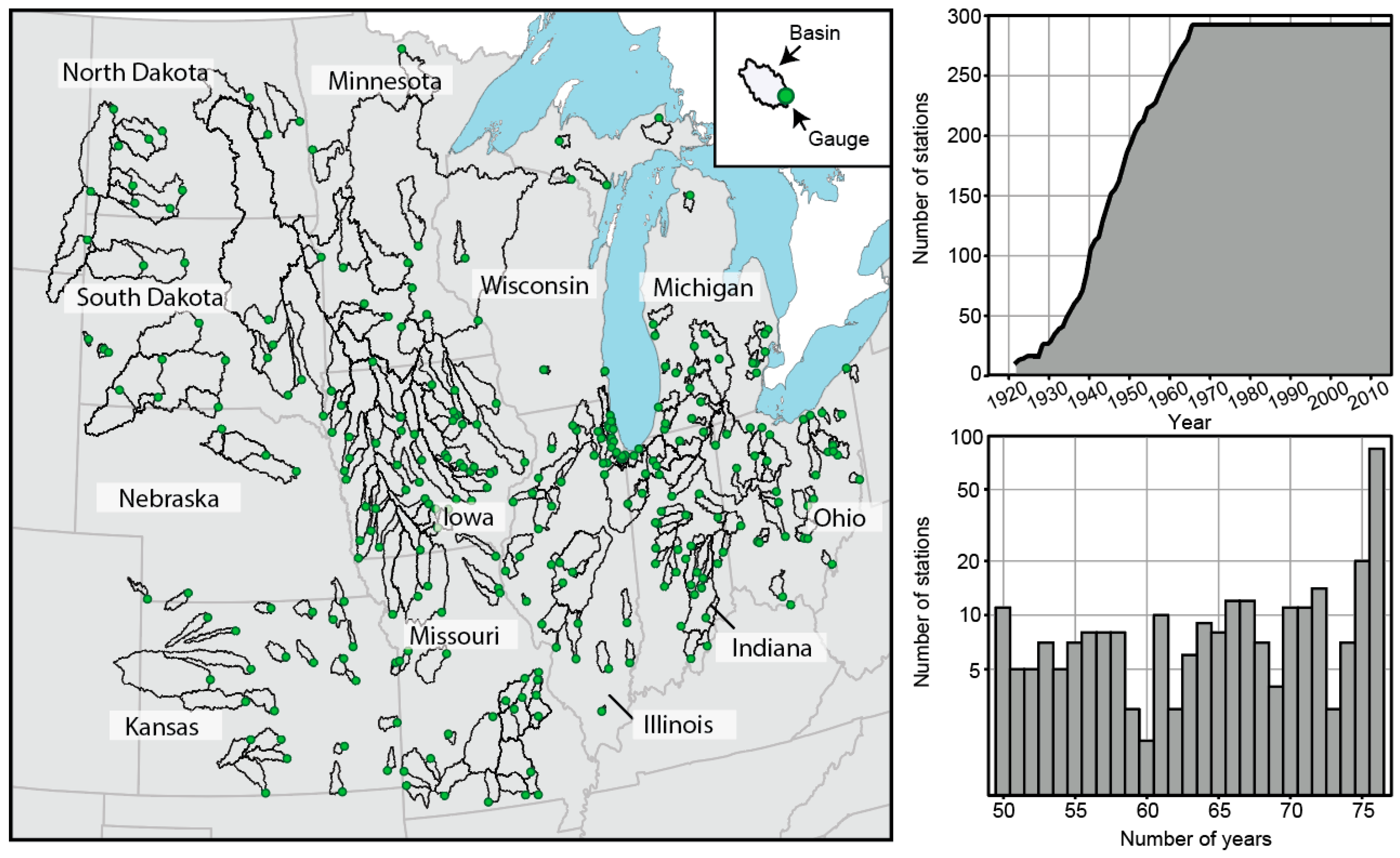
Figure 1. Location of the 290 study sites and their contributing drainage basins across the Midwest. Contributing drainage basins are outlined in black and may extend beyond the region that is shown in the figure. The top right panel shows the number of stations with complete data in every year (a continuous record of at least 50 years before 2015 is required). The bottom right panel shows the histogram of record length for the 290 stations.
Water 09 00695 g001
Figure 2. Location of agricultural and urban drainage basins. Gauging stations are indicated as red circles, and contributing drainage basins as black outlines: (Left) percent of the basin that is planted as corn and soybean in 2014, ranging from yellow (0–5%) to dark green (>95%); (Right) urban areas (blue) and urban drainage basins (with a population density of more than 50 persons/km2).
Water 09 00695 g002
Figure 3. Examples of one agricultural and one urban site: (Left) South Raccoon River at Redfield, Iowa (agricultural); (Right) Du Page River at Shorewood, Illinois (urban). Rows indicate time series of five basin-averaged predictors (1940–2015). Row 1: Agricultural land cover (% of basin; black circles); the horizontal black line shown at 33% is the cut off point for selecting agricultural basins. Row 2: Population density (persons/km2); the horizontal line shown at 50 persons/km2 is the cutoff point for selecting urban basins. Row 3: Streamflow quantiles ranging from Q0 to Q1, with a step of 0.05, on a logarithmic scale. Row 4: Total seasonal precipitation (mm). Row 5: Mean seasonal temperature (°C). In Rows 4 and 5, each season is shown with a different symbol: winter (pluses), summer (squares), spring (triangles), and fall (circles). See Figure S1 for plots of streamflow and predictors at all 290 sites.
Water 09 00695 g003
Figure 4. Time series illustrating probabilistic model fits at two sites (1940–2015): model P.PA at the South Raccoon River at Redfield, Iowa (site 05484000), and model P.Ppop at the Du Page River at Shorewood, Illinois (site 05540500). Two seasons are shown: spring (top); and summer (bottom). Within each panel, the rows correspond to three streamflow quantiles: low flow (Q0.05), median flow (Q0.5) and high flow (Q0.95). The fitted distribution is shown in three colors: a pale blue ribbon (5th–95th percentiles), a dark blue ribbon (25th–75th percentiles), and a white line passing through the middle (50th percentile). The white-filled circles indicate the observed values. For time series of model fits at all other sites, see Figure S2.
Water 09 00695 g004
Figure 5. Best-fitting model selection, by flow quantile and season. For every measured quantile, within every season, we compute the number of times (%) that each of the seven models was selected (based on the smallest AIC of the models that were fit for the given site, season and flow quantile). Thus, for example, for the summer low flows (Q0), P.PA.M was the best-fitting model at 31% of the sites. The four panels indicate the seasons, rows indicate the seven models, and colors indicate the number of times that each model was selected for the given quantile, ranging from less than <5% (yellow) to >45% (dark orange). Grey indicates that the model was not available for selection (Mixed model in winter) or that no sites were selected. The absolute number of sites where the given model was selected is indicated within each color box.
Water 09 00695 g005
Figure 6. Best-fitting model, by quantile and season. Colored circles indicate the best-fitting model based on the smallest AIC for all of the models that were fit at every site. Rows indicate the four seasons (winter, spring, summer and fall), and columns the three selected flow quantiles for low, median and high flow (Q0.05, Q0.5, and Q0.95). The models are indicated as: yellow (Mixed model), blue (P), orange (P.M), green (P.PA), magenta (P.PA.M), black (P.Ppop) and red (P.T). For maps of the best-fitting models for every one of the 21 flow quantiles and for every season, see Figure S3.
Water 09 00695 g006
Figure 7. Correlation coefficient for the best-fitting model at each site. Each panel indicates the correlation coefficient between the best model’s median and observations, as indicated in Figure 5, by flow quantile and season. The legend indicates the value of the correlation coefficient (R) ranging from blue (−1) to red (1), with values centered around 0 shown in white (−0.025 to +0.025). The fits for the best models at each site are shown in the Figure S2. For comparison, Figure S6 shows the same information as Figure 7 but computed with Spearman’s rho instead of Pearson’s correlation coefficient R (nonparametric equivalent).
Water 09 00695 g007
Figure 8. Correlation coefficient for the best-fitting model at each site based on cross-validation, shown by flow quantile and season. The symbology is the same as in Figure 7, to facilitate the comparison between the model fit and the cross-validation. Cross-validation is shown for all quantiles in Figure S5. For comparison, Figure S7 shows the same information as Figure 8 but computed with Spearman’s rho instead of Pearson’s R (nonparametric equivalent).
Water 09 00695 g008
Figure 9. Influence of additional predictors on model fits. The fits are assessed here using the correlation coefficient (R) at all models where model P is not the best fit (18,815 model fits, across every site, flow quantile and season). The four panels indicate the four seasons: within each panel, the boxplots on the left indicate the correlation coefficient for Model P; those on the right indicate the correlation coefficient for the best-fitting model at each site (i.e., with additional predictors). The top right panel shows the absolute difference between the correlation coefficients (𝛿R) for the best-fitting model and Model P at each site. For comparison, Figure S8 shows the same information as Figure 9 but computed with Spearman’s rho instead of Pearson’s correlation coefficient R (nonparametric equivalent). [Note that this figure indicates R for the models, not the CV.]
Water 09 00695 g009
Figure 10. Sensitivity analyses for three models based on a change in each predictor (precipitation, population density or agriculture) within three models: P, P.Ppop and P.PA. The four panels indicate a change in each predictor of +10%, +5%, −5% and −10%, from top to bottom. Within each panel, spring and summer seasons are shown (top and bottom, respectively). All streamflow quantiles are shown (x-axis). The percent change in streamflow resulting from a given change in each of the predictors is indicated in colors ranging from dark blue (strong decrease in streamflow) to dark red (strong increase in streamflow).
Water 09 00695 g010
Table 1. Description of the seven models, their predictors and formulation.
Model AcronymPredictorsModel Formulation#
P x p : precipitation { l o g ( μ 1 ) = α 1 + β 1 · x p l o g ( σ 1 ) = κ 1 1
P.T x t : temperature { l o g ( μ 2 ) = α 2 + β 2 · x p + γ 2 · x t l o g ( σ 2 ) = κ 2 2
P.M x m : antecedent wetness { l o g ( μ 3 ) = α 3 + β 3 · x p + γ 3 · x m l o g ( σ 3 ) = κ 3 3
P.PA x a : agricultural land cover (%) { l o g ( μ 4 ) = α 4 + β 4 · x p + γ 4 · x p · x a l o g ( σ 4 ) = κ 4 4
P.Ppop x p o p : population { l o g ( μ 5 ) = α 5 + β 5 · x p + γ 5 · x p · x p o p l o g ( σ 5 ) = κ 5 5
P.PA.Mas above { l o g ( μ 6 ) = α 6 + β 6 · x p + γ 6 · x p · x a + δ 6 · x p · x m l o g ( σ 4 ) = κ 6 6
Mixed (spring) x t m a r a p r : mean March–April temperature { l o g ( μ 7 , s p r i n g ) = α 7 + β 7 · x p + γ 7 · x m + δ 7 · x t m a r a p r l o g ( σ 7 , s p r i n g ) = κ 7 7a
Mixed (summer and fall) x t s u m m e r : mean June–August temperature { l o g ( μ 7 , s u m m e r / f a l l ) = α 7 + β 7 · x p + γ 7 · x m + δ 7 · x t s u m m e r l o g ( σ 7 , s u m m e r ) = κ 7 7b