Agreement of Four Equations for Computing Dewfall in Northern Germany

Abstract

The energy balance (EB), turbulent vapour transport (TVT), Penman-Monteith (PM) and Bowen ratio energy balance (BREB) equation were used to estimate dewfall based on meteorological data. Initially there were big disagreements between the estimates from these four equations. However, after multiplying the heat and vapour conductance terms by 0.33 the agreement was much better. This implies that the disagreements derived from improper conductance values. Initially we did not consider the effect of atmospheric stability on the conductances. With stability correction the conductances were on average 0.5 times the values without stability correction. To arrive at the aforementioned 0.33, the conductances with stability correction still need to be lower by a factor of 0.66. The value of the von Karman constant and the relationships for the zero plane displacement and the roughness length we used in our conductance computations are widely used, but not the only possible ones. With different values and relationships also suggested in the literature one can reach this factor. However, it is also possible that our wind speed data contributed to the fact that the conductances we computed were too high. Their computation for a given canopy—atmosphere system requires wind speeds from a wind profile in equilibrium with the vegetation. This in turn requires an adequate fetch around the investigated surface. The highly varied vegetation in and around the site where the study was conducted makes adequate fetch rather doubtful. To obtain valid conductance values the atmospheric stability conditions must be considered, the appropriate values for the von Karman constant, the zero plane displacement and roughness length must be used, and there must be adequate fetch. The BREB equation does not contain a conductance term and therefore does not suffer from the problems just stated. The other three equations do. However, the BREB, like the EB and TVT equations, need the surface temperature which is not routinely measured. This then leaves the PM equation from which this temperature has been eliminated as the only option. Hence, in a future study dewfall estimates from the PM equation should be compared with direct measurements with a high precision weighing lysimeter.

1. Introduction

Water vapour condensed on the surface of an object is referred to as dew. Dew occurs only when the surface temperature drops to or below the dew point temperature of the ambient air. Dew is a form of precipitation. However, it is usually ignored because of its small amount which is normally in the range 0.3–0.5 mm per night [1]. While dew contributes only a small percentage to the annual precipitation in most regions of the world, it is an important water supply for plants in some arid regions [2,3,4]. In addition, some studies show that dew can contribute to the stabilisation of sand dunes [5,6]. Dew can also improve the internal water balance of plants [7,8,9,10], prolong the survival of tree seedlings [11,12], and delay the wilting of leaves [11].

Dew amounts can be measured with various dew gauges, but there is still no standard method of measurement. Lysimeters are a very promising tool to quantify dewfall [13]. However, they are not widespread, because they are expensive. Hence, one often needs to consider other ways to determine dewfall. One alternative is to compute it from meteorological data under consideration of the properties of the surface [14,15,16]. Dewfall represents a flux of latent heat towards the surface, the opposite of evaporation. It is therefore possible to compute the amount of dew formation with methods developed for computing evaporation. Based on these methods there is a large body of literature on computing dew formation. The most widely used methods are the energy balance (EB), turbulent vapour transport (TVT), Penman-Monteith (PM) and Bowen ratio energy balance (BREB) equation.

Since dewfall represents a latent heat flux at a surface, it can be estimated from the energy balance of an atmosphere–canopy system, if the other components of the EB are available either from measurement or calculation [17,18,19,20,21]. Dewfall estimated with the EB equation is generally in good agreement with measurements.

The TVT equation was developed by [14] and applies the principles of turbulent transport to water vapour. Using routine meteorological data it can estimate dewfall on grass or bare surfaces. Ref. [14] found that dewfall estimated with this equation was close to that measured by a dew gauge at the same site.

The PM equation was originally developed to calculate evaporation and transpiration, but is now also used to estimate dewfall [22]. This equation takes into account the transport of energy and vapour in the atmosphere. It has been applied to studies of dew formation on various types of vegetation and in different regions [1,3,23,24,25,26,27,28]. The results have proven that the PM equation can estimate dewfall with high precision.

Finally, the BREB equation was developed based on the EB equation. It was simplified by introducing a ratio into the equation [29] which eventually became known as the Bowen ratio. The BREB equation was successfully used to determine above-crop vapour flux towards the canopy, i.e., dewfall [30,31,32].

In previous studies estimates from these equations were usually compared with different measurements rather than each other. For example, the BREB equation was tested against an eddy covariance system, and latent and sensible heat fluxes from both were in good agreement [33]. Likewise, the EB equation was tested against a microlysimeter, and calculated dewfall amounts gave reasonable estimates of daily dewfall [34]. The objective here is to compare dewfall estimated with these equations and evaluate their performance. We shall then discuss possible reasons for differences in the estimates and ways to overcome them. Finally, we shall identify the equation most suitable for everyday use.

2. Materials and Methods

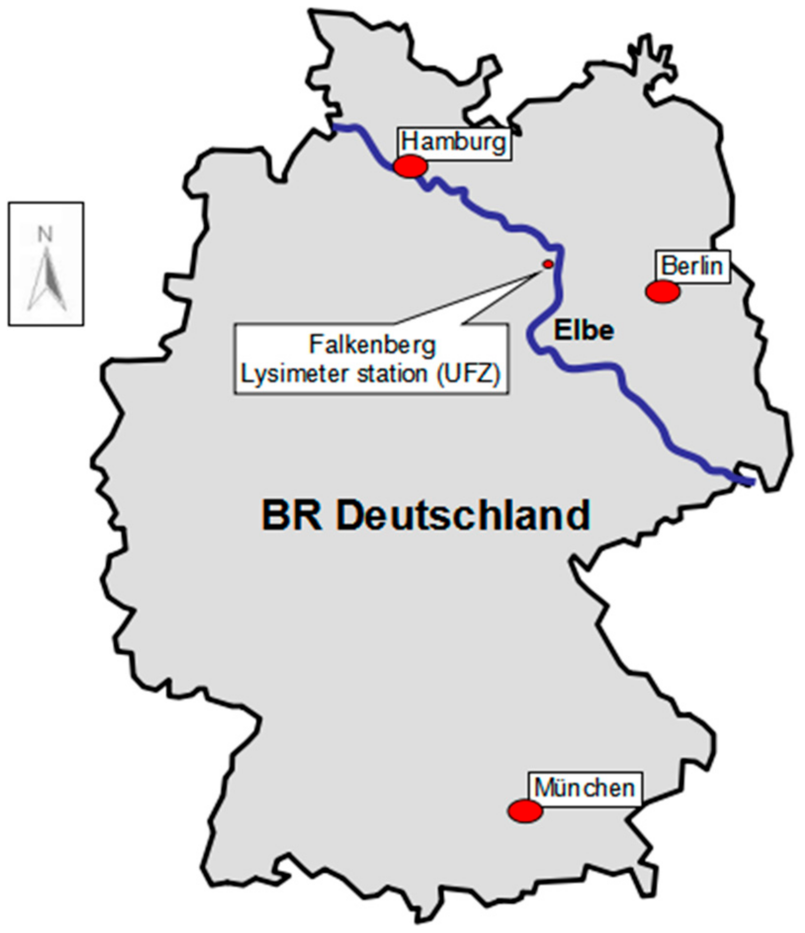
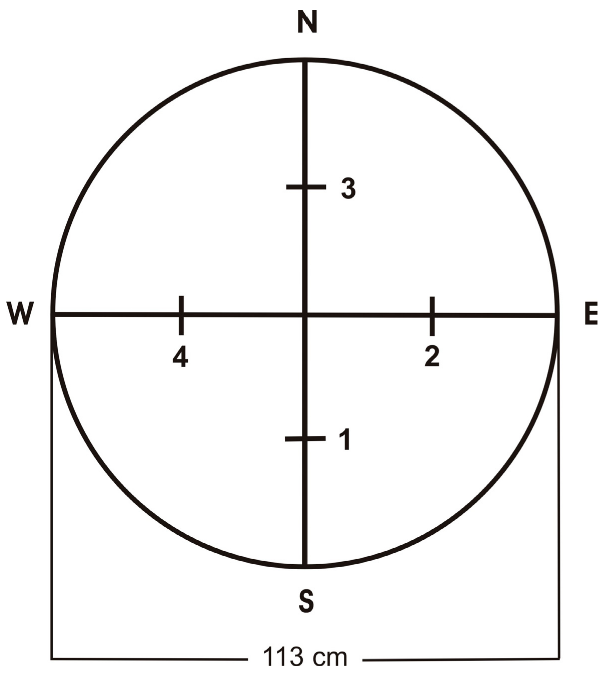
2.1. Data Collection

The computations were made for a 20 cm tall grass surface at the Falkenberg lysimeter station of the Helmholtz Centre for Environmental Research which is located some 120 km northwest of Berlin, Germany (Figure 1). The site is 21 m above sea level, its mean annual precipitation is 588 mm with a maximum in July (69 mm) and a minimum in February (29 mm). Its potential annual evapotranspiration is 565 mm, also with a maximum in July (106 mm) and a minimum in February (8 mm). The surrounding area is plain and mainly under grassland [13].

The necessary meteorological data were collected from 19 to 21 November 2009. Air temperature was measured 2 m above ground over a grass surface with platinum resistance elements (809 LO-100, Wilh. Lambrecht GmbH, Göttingen, Germany) ventilated in an Assmann psychrometer shield. Relative humidity was measured at the same height with a shielded sensor (Mela CPC1/5-ME, MELA Sensortechnik GmbH, Mohlsdorf, Germany). Wind speed was measured with a cup anemometer (Wind Sensor Meteorology 14576-24V, Wilh. Lambrecht GmbH, Göttingen, Germany) at 10 m height. These measurements were logged automatically as 10 min averages throughout the day. Two temperature sensors (Pt100, Temperaturmeßtechnik Geraberg, Martinroda, Germany) were buried at 5 cm and 10 cm depth, respectively, and a thermal conductivity probe (Thermolink, Decagon Devices, Pullman, WA, USA) was buried at a depth of 7.5 cm to compute soil heat flux. Soil temperature and thermal conductivity were recorded every half hour.

Net radiation was measured with a net radiometer (NR Lite, Kipp and Zonen, Delft, The Netherlands) at 1 m height above the 20 cm tall grass and recorded every ten minutes. Canopy surface and in-canopy temperature of the grass were measured hourly at four different positions in a 1 m² circular sample plot (Figure 2) with a hand-held infrared thermometer (Raynger MX4, Raytek Corporation, Santa Cruz, CA, USA). Surface emissivity was set to 0.95, which is a typical value for soils and plants [35]. Cloud cover was estimated visually every hour. It is not required for the computations, but a useful parameter to interpret the net radiation data.

2.2. Equations

The four equations used here are introduced below. Following convention, all equations are written such that fluxes towards the surface are positive. For a detailed derivation the reader is referred to [36] or the Appendix A.

Energy balance equation (EB):

$$E=-\hspace{0.17em}\left(R_n+G+H\right)=-R_n-k_T\cdot \frac{T_{10}-T_5}{\Delta z}-g_h\cdot c_p\cdot \left(T_a-T_s\right)$$

(1)

Equation for turbulent vapour transport (TVT):

$$E=\lambda \cdot g_v\cdot \frac{\left[e_a-e_s(T_s)\right]}{P}=\lambda \cdot g_v\cdot \frac{h_r\cdot a\cdot \exp \hspace{0.17em}\left(\frac{b\cdot T_a}{T_a+c}\right)-a\cdot \exp \hspace{0.17em}\left(\frac{b\cdot T_s}{T_s+c}\right)}{P}$$

(2)

Penman-Monteith equation (PM):

$$E=\frac{-s\cdot \left[R_n+G\right]+g_v\cdot c_p\cdot \left[e_a-e_s(T_a)\right]}{s+\frac{c_p\cdot P}{\lambda }}=\frac{-\frac{b\cdot c\cdot e_s(T)}{\left(c+T\right){ }^2}\cdot \left[R_n+G\right]+g_v\cdot c_p\cdot \left[e_a-e_s(T_a)\right]}{s+\frac{c_p\cdot P}{\lambda }}$$

(3)

Bowen ratio energy balance equation (BREB):

$$E=-\frac{R_n+G}{\left(1+\beta \right)}=-\frac{R_n+G}{\left(1+\frac{c_p\cdot P}{\lambda }.\frac{\left[T_a-T_s\right]}{\left[e_a-e_s(T_s)\right]}\right)}$$

(4)

where E = latent heat flux between atmosphere and surface (W·m⁻²), R_n = net radiation (W·m⁻²), G = soil heat flux (W·m⁻²), H = sensible heat flux between atmosphere and surface (W·m⁻²), k_T = thermal conductivity of the soil (W·m⁻¹·°C⁻¹), T₁₀ = soil temperature at 10 cm depth (°C), T₅ = soil temperature at 5 cm depth (°C), Δz = distance between the two soil temperature probes (m), g_h = heat conductance of the air between the surface and screen height (mol·m⁻²·s⁻¹), c_p = heat capacity of air (J·mol⁻¹·°C⁻¹), T_a = air temperature (°C), T_s = surface temperature (°C), λ = latent heat of vaporization (J·mol⁻¹), g_v = vapour conductance of the air between the surface and screen height (mol·m⁻²·s⁻¹), e_a = vapour pressure of the ambient air (Pa), e_s (T_s) = saturation vapour pressure of the air at surface temperature (Pa), P = air pressure (Pa), h_r = relative humidity of the air (dimensionless fraction), a = 611 Pa, b = 17.502 (dimensionless), c = 240.97 °C, s = slope of the temperature—saturation vapour pressure curve (Pa·°C⁻¹), e_s (T_a) = saturation vapour pressure of the air at air temperature (Pa), T = mean of air and surface temperature (°C), and β = Bowen ratio (dimensionless).

Note that in the Penman-Monteith equation s is usually evaluated at air temperature. This introduces some error. It is more precise to use the average of air and surface temperature. Since in our case the surface temperature was known, we employed this average temperature.

We calculated g_h and g_v following [35] as:

$$g_h=g_v=\frac{k^2\cdot {\rho }_a\cdot u}{\ln \hspace{0.17em}\left(\frac{z-d_m}{z_m}\right)\cdot \ln \hspace{0.17em}\left(\frac{z-d_{hv}}{z_{hv}}\right)}$$

(5)

where k = von Karman constant (here 0.4, dimensionless), ρ_a = molar density of air (mol·m⁻³), u = wind speed at height z (m·s⁻¹), z = height of wind speed measurement (m) = screen height, d_m = zero plane displacement for mechanical energy (m) = 0.65·h, z_m = roughness length for mechanical energy (m) = 0.1·h, d_hv = zero plane displacement for heat and vapour movement (m) = 0.6·h, z_hv = roughness length for heat and vapour movement (m) = 0.02·h, and h = canopy height (m). As most people do, [35] assume that the heat and vapour conductance are equal.

3. Results

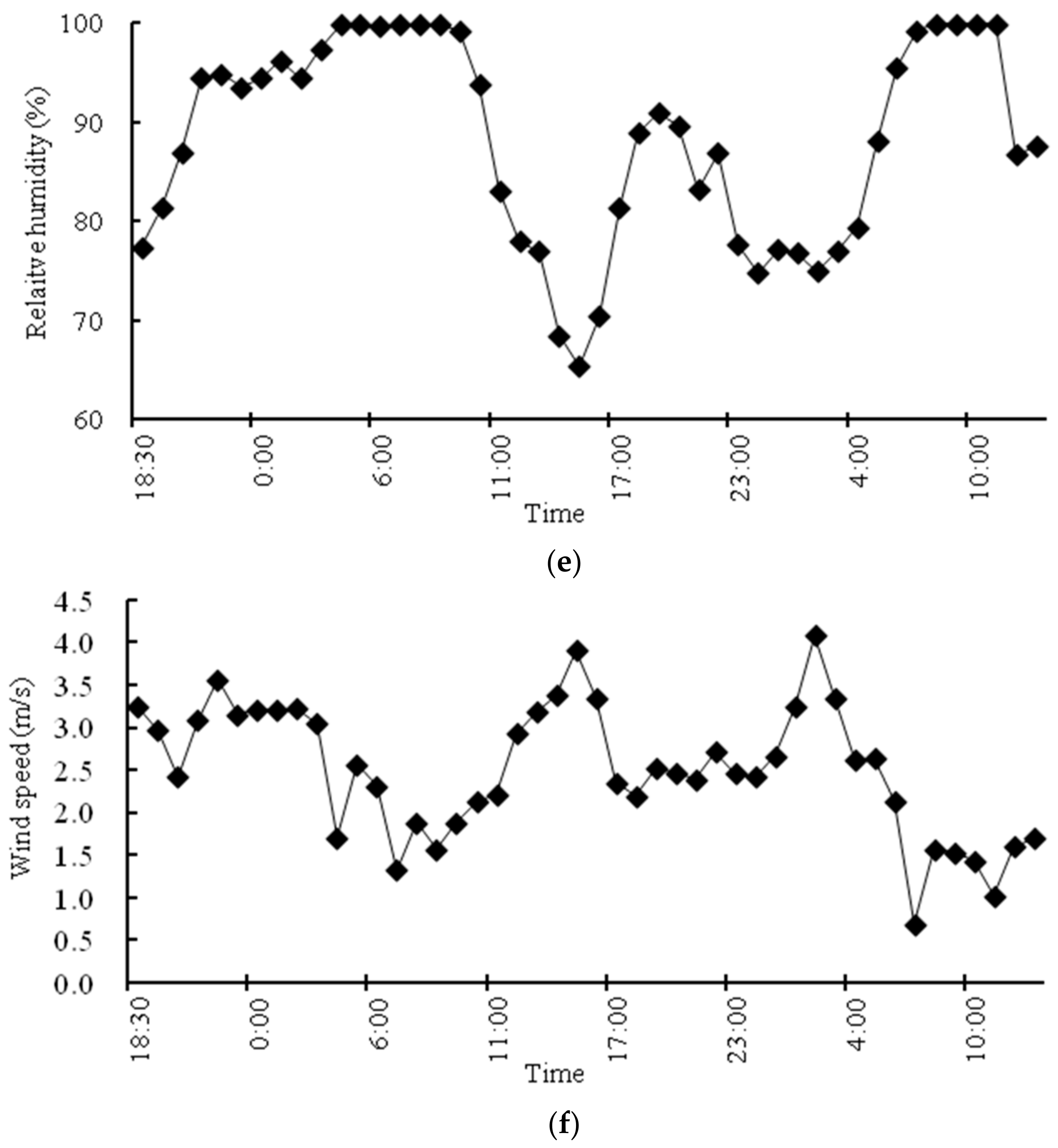
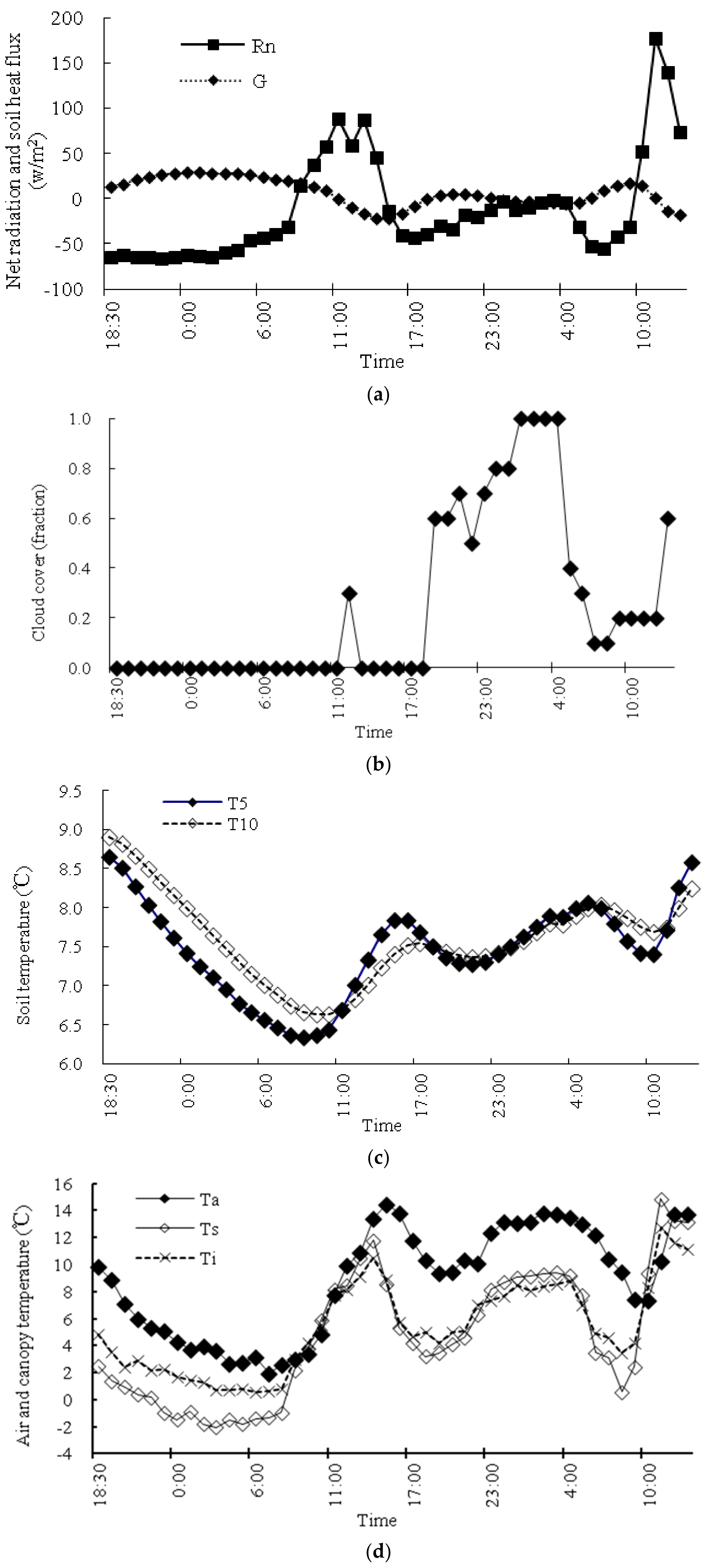
3.1. Meteorological Data

Figure 3 displays the changes in net radiation (R_n), soil heat flux (G), cloud cover, soil temperature at 5 and 10 cm depth (T₅ and T₁₀), air (T_a), canopy surface (T_s) and in-canopy (T_i) temperature, relative humidity, and wind speed from 18:30 on 19 November to 13:00 on 21 November 2009. As state above, any flux towards the surface is given as a positive value, and any flux away from it as a negative value.

Net radiation R_n was directed away from the surface (negative) during the first night (Figure 3a). It remained more or less constant for most of the night, but then increased slowly as sunrise approached. It became positive around 8:30 and then increased rapidly towards a peak around midday from where it decreased again. By 15:00 it was negative. The dip at midday was caused by a brief rise in cloud cover (Figure 3b). At 18:00 on the second night cloud cover increased markedly. In line with this, R_n became less negative and approached zero, because the clouds diminished the radiation loss. At 4:00 cloud cover decreased markedly and R_n became more negative again. As the sun came up R_n increased steeply until 11:00 and then fell due to another increase in cloud cover.

The variations in soil temperature and the associated soil heat flux generally responded to the evolution of R_n (Figure 3c). During the first night the negative R_n resulted in an energy loss and soil temperature decreased. Temperature changes first occurred near the surface and, after a time lag, at greater depths. Hence, T₅ was significantly less than T₁₀ which gave rise to a distinct soil heat flux towards the soil surface (Figure 3a). In the second night the soil temperatures at 5 and 10 cm depth were fairly similar during the hours with cloud cover >0.6 (Figure 3b) when radiation loss was reduced. As a result, there was little soil heat flow in either direction (Figure 3a). At 4:00 the clouds began to disappear, so radiation loss increased again (Figure 3a). This in turn caused T₅ to fall below T₁₀ so that a distinct soil heat flux towards the soil surface developed.

Nightly air temperature (T_a) was always higher than the surface temperature of the grass (T_s) during the night of 19–20 November (Figure 3d). The temperature inside the grass canopy (T_i) was always higher than that at the canopy surface (T_s), too, because of radiative heat loss from the canopy surface and heat gain from G inside the canopy. During most of the day on 20 November T_s was slightly greater than T_i, because of radiation gain at the canopy surface and some heat loss to the soil from inside the canopy. From sunrise on November 20 until the early afternoon T_a rose and then declined again until 19:00, when the decline was first halted due to increasing cloudiness, which reduced radiation loss, and later even reversed as a result of warm air moving across the area. The disappearance of the clouds and of the warm air after 4:00 led to an increase in radiation loss and, consequently, to falling temperatures. They began to climb again sometime after sunrise as R_n increased. T_a was always above T_s in the night of 20–21 November, too. T_s was above T_i during the hours when the warm air moved across and cloudiness was high. In the other night hours T_s was below T_i.

During the first night, relative humidity increased as the air cooled (Figure 3e). It reached almost 100% around 4:00 and remained at that level until warming after sunrise. With the rise in air temperature the relative humidity dropped until 16:00. Thereafter it rose again as the air cooled. This rise was stopped at 19:00 due to increasing cloudiness and later reversed as the warm air passed by. After 4:00, when the clouds and the warm air had gone, relative humidity quickly increased to nearly 100%.

Wind speed is displayed in Figure 3f. It was quite low during the whole period and shows no distinct pattern.

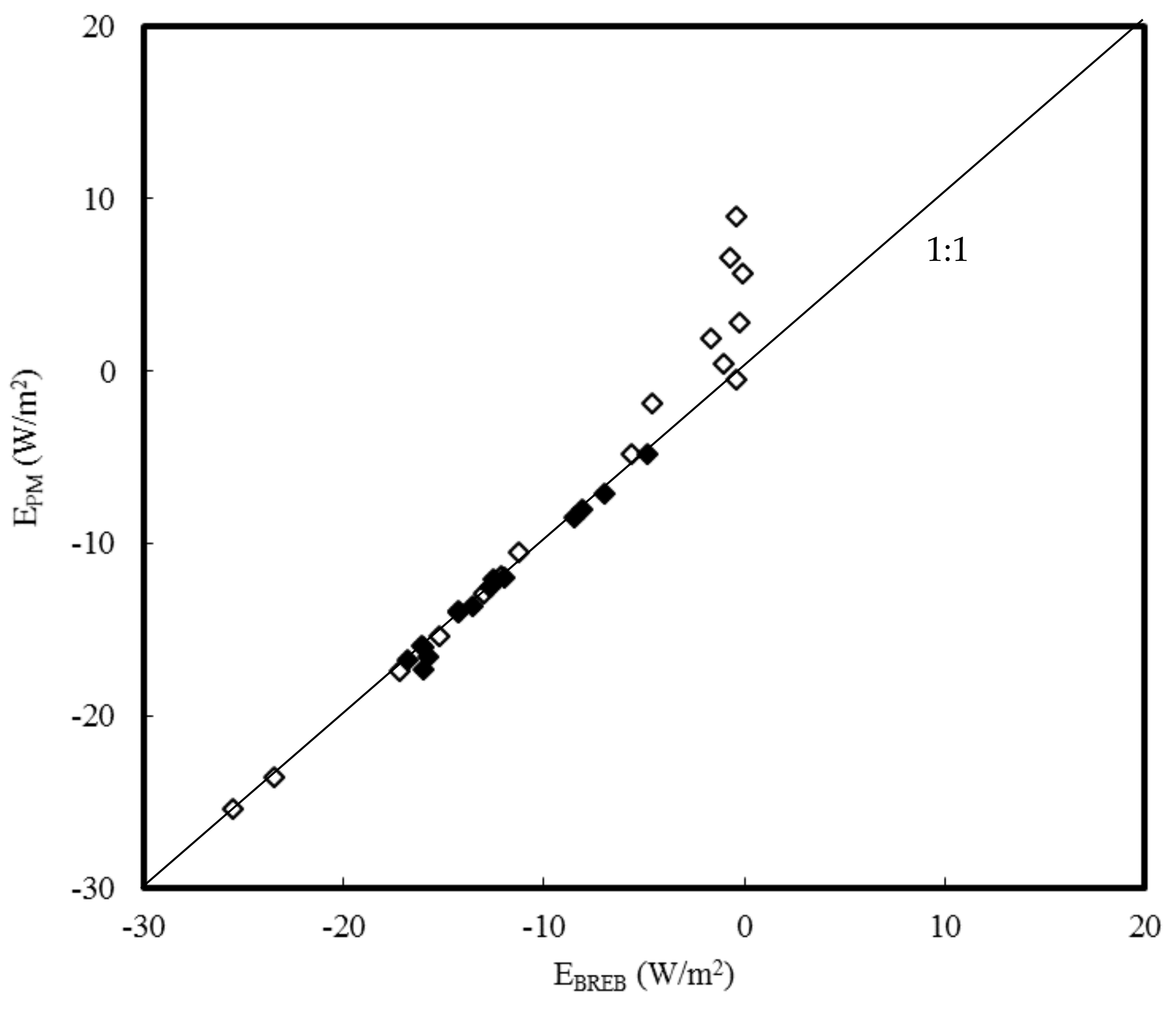
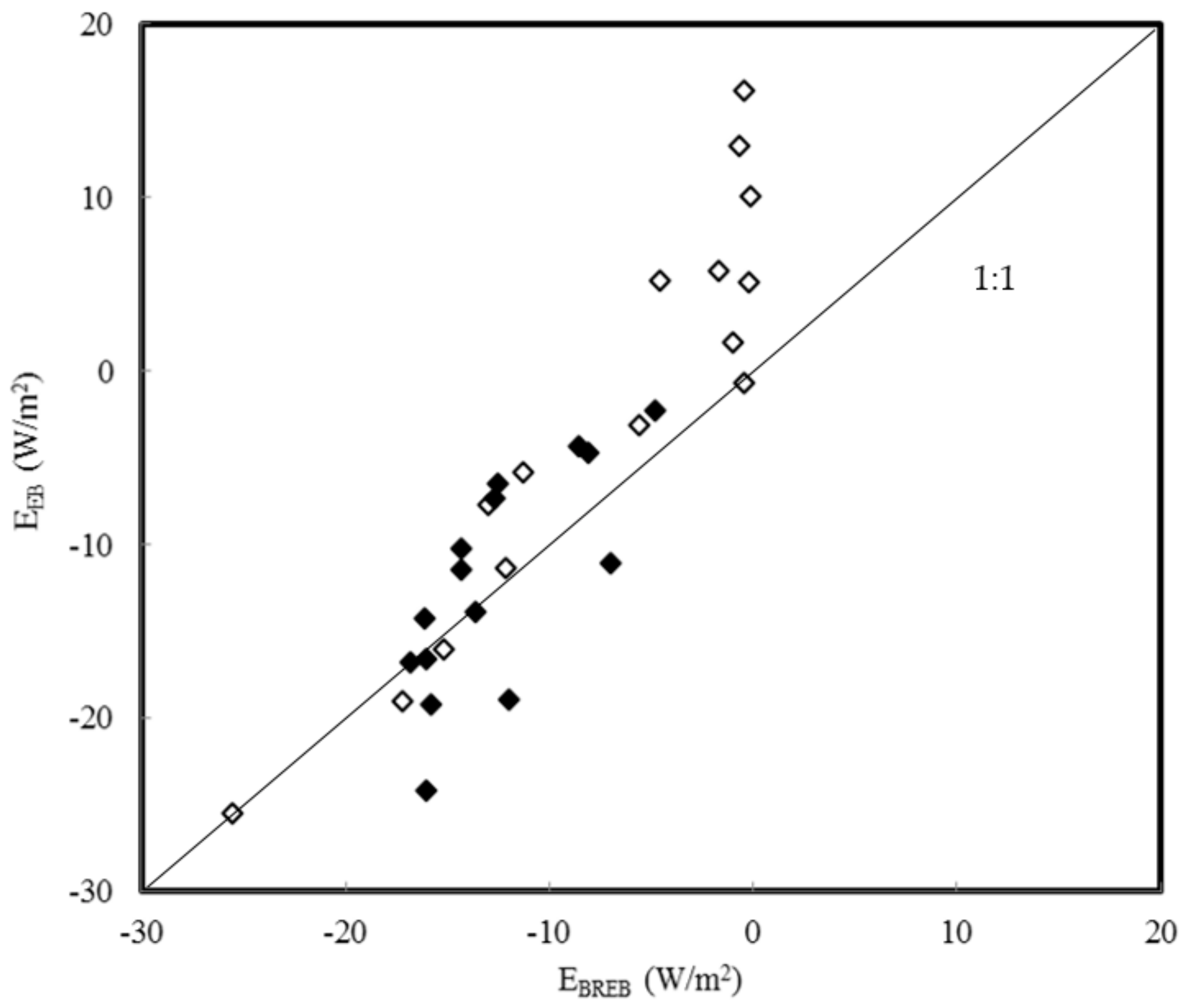
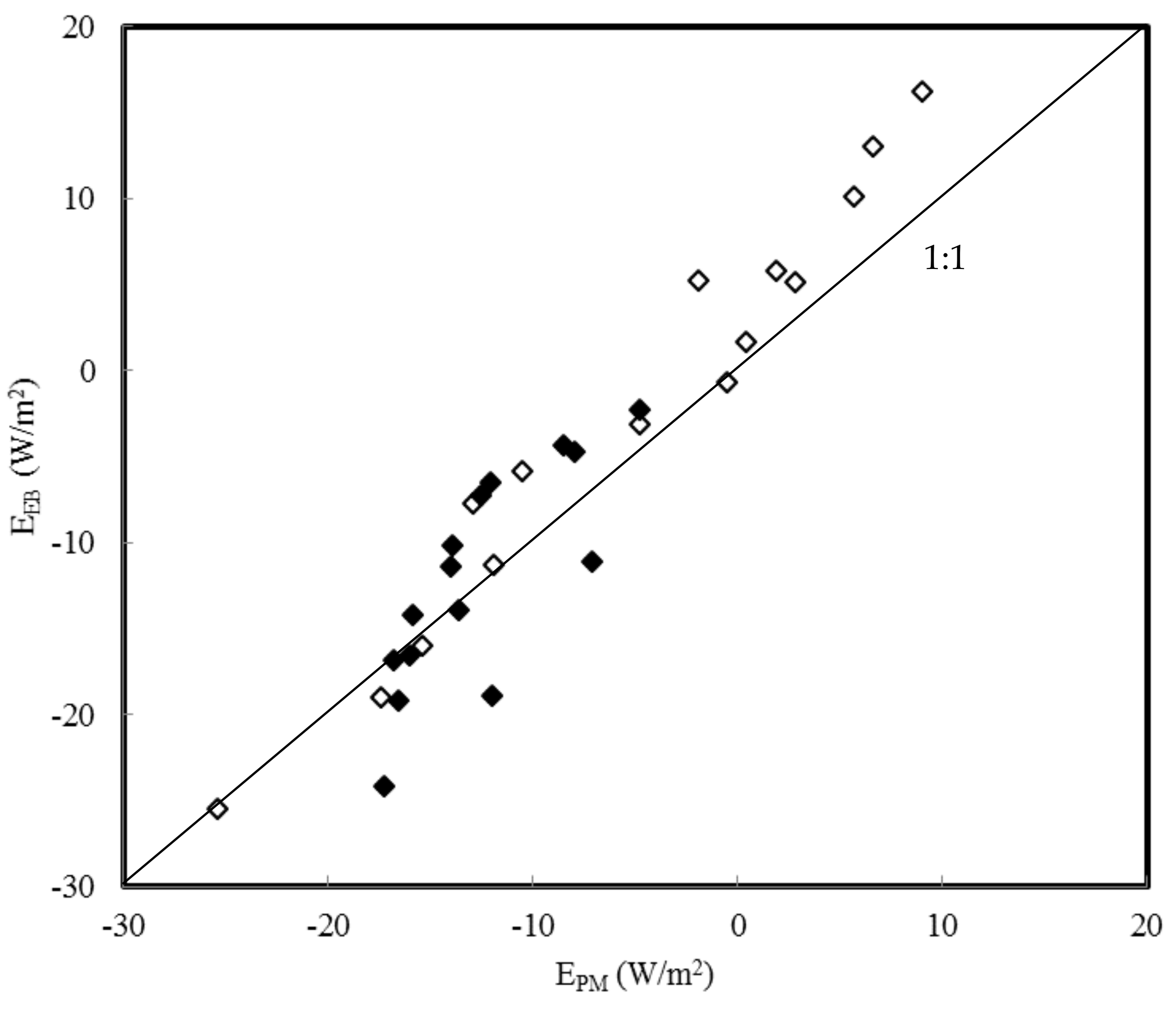
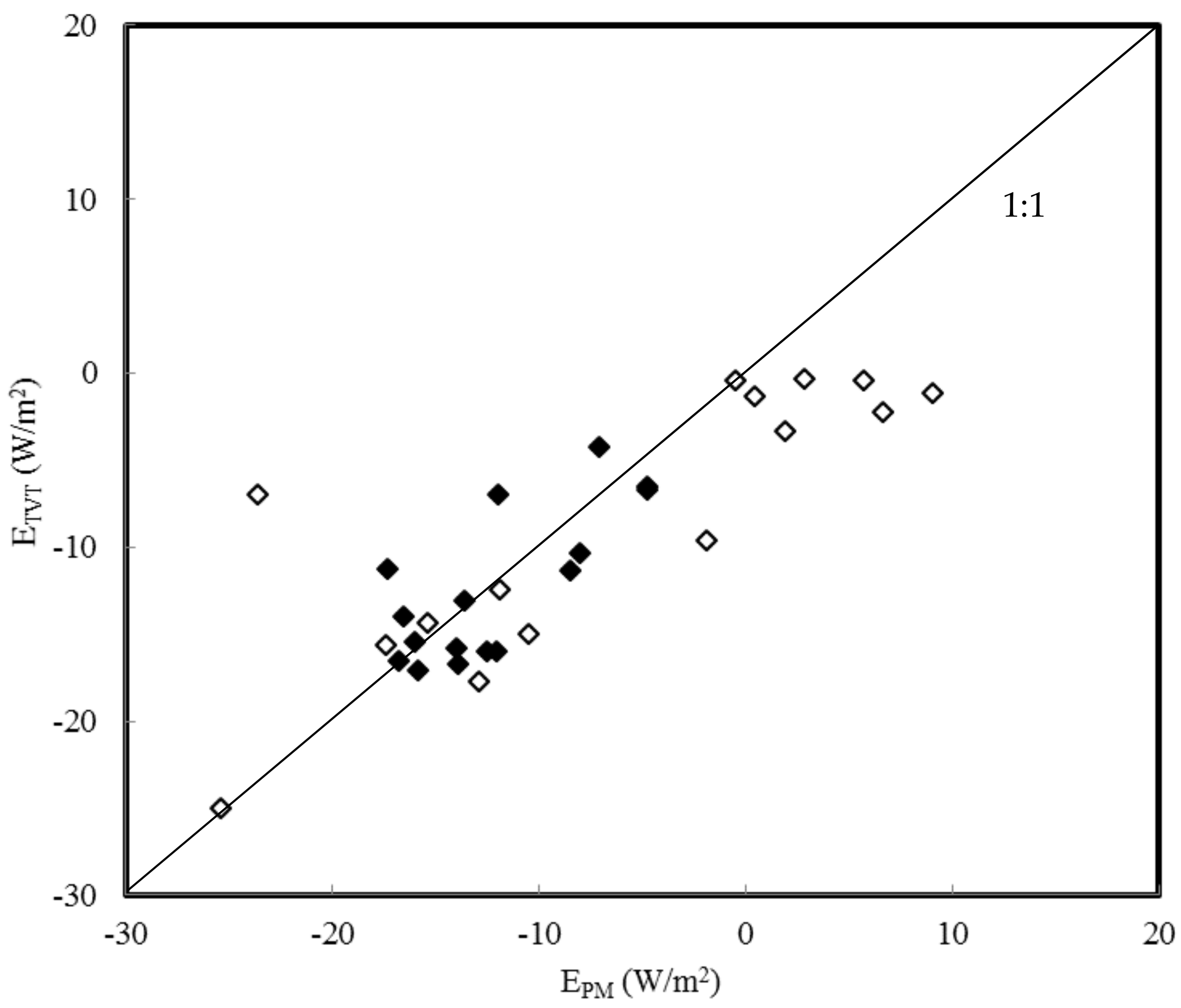
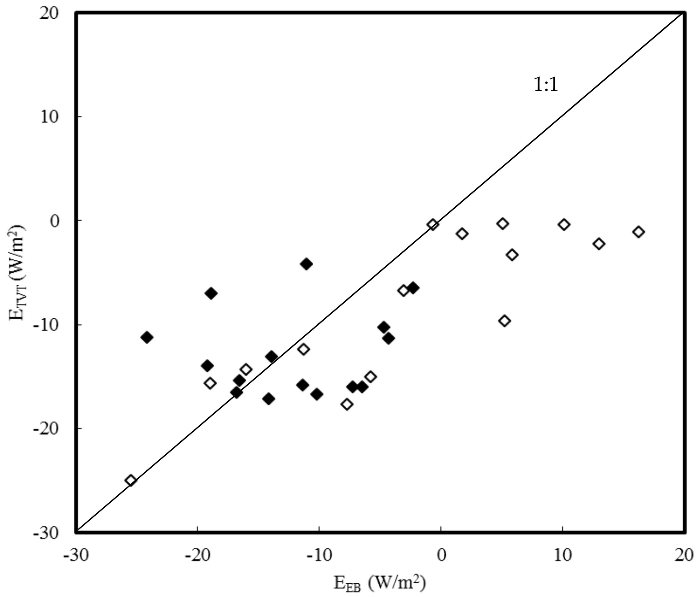
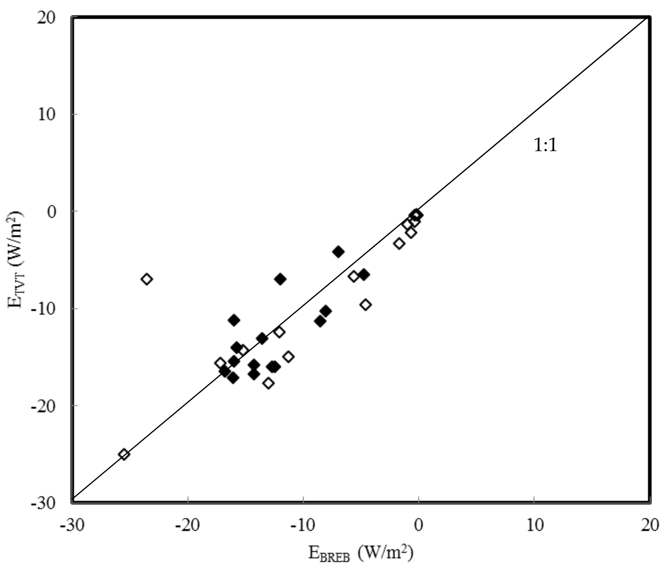
3.2. Performance of the Equations

Due to the varying assumptions implied in the equations, they cannot be expected to produce exactly the same values, but they should be similar. Columns 2 to 5 in

Table 1. Dewfall (latent heat flux) estimated with the energy balance (E_EB), turbulent vapour transport (E_TVT), Penman-Monteith (E_PM), and Bowen ratio energy balance (E_BREB) equation. Columns 2–4 are without, and columns 8–10 with adjustment of the heat and vapour conductance computed with Equation (5) by a factor of 0.33. The E_BREB values are given again in column 11 for easier comparison. Also presented are the conductances computed with Equation (5) (g), and the conductances computed with a stability correction in Equation (5) (g_Ψ).

Time	EEB	ETVT	EPM	EBREB	g	gΨ	EEB	ETVT	EPM	EBREB
	W/m2	W/m2	W/m2	W/m2	mol/m2/s	mol/m2/s	W/m2	W/m2	W/m2	W/m2
Data for 18:30 on 19 November to 8:00 on 20 November 2009
18:30	47.2	−42.4	2.4	−15.8	0.467	0.234	−19.2	−14.0	−16.6	−15.8
19:00	45.5	−46.7	−2.1	−16.0	0.429	0.203	−16.6	−15.4	−16.0	−16.0
20:00	17.7	−34.1	−10.0	−16.0	0.351	0.154	−24.2	−11.2	−17.3	−16.0
21:00	32.2	−50.1	−13.0	−16.8	0.450	0.238	−16.8	−16.5	−16.8	−16.8
22:00	37.8	−51.8	−12.0	−16.1	0.519	0.306	−14.2	−17.1	−15.9	−16.1
23:00	43.9	−50.5	−9.6	−14.3	0.461	0.240	−10.2	−16.7	−13.9	−14.3
0:00	46.2	−48.5	−8.3	−12.5	0.470	0.252	−6.5	−16.0	−12.1	−12.5
1:00	28.0	−39.8	−11.2	−13.6	0.469	0.268	−13.9	−13.1	−13.6	−13.6
2:00	41.5	−47.8	−10.4	−14.3	0.472	0.253	−11.4	−15.8	−14.0	−14.3
3:00	42.3	−48.4	−10.8	−12.7	0.446	0.232	−7.3	−16.0	−12.5	−12.7
4:00	1.5	−21.1	−11.9	−12.0	0.251	0.099	−18.9	−7.0	−12.0	−12.0
5:00	29.1	−34.3	−8.4	−8.5	0.378	0.190	−4.3	−11.3	−8.5	−8.5
6:00	25.1	−31.1	−7.9	−8.1	0.339	0.159	−4.7	−10.3	−8.0	−8.1
7:00	1.4	−12.6	−7.0	−7.0	0.196	0.070	−11.1	−4.2	−7.1	−7.0
8:00	16.7	−19.8	−4.8	−4.8	0.278	0.124	−2.3	−6.5	−4.8	−4.8
Data for 18:00 on 20 November to 8:00 on 21 November 2009
18:00	24.3	−47.3	−11.0	−17.2	0.315	0.123	−19.0	−15.6	−17.4	−17.2
19:00	35.9	−45.6	−4.7	−11.3	0.363	0.166	−5.8	−15.0	−10.5	−11.3
20:00	25.6	−37.6	−5.6	−12.1	0.355	0.166	−11.3	−12.4	−11.9	−12.1
21:00	43.2	−29.1	8.4	−4.6	0.343	0.154	5.2	−9.6	−1.9	−4.6
22:00	25.7	−20.4	4.0	−5.6	0.388	0.214	−3.1	−6.7	−4.8	−5.6
23:00	29.7	−3.9	15.0	−1.0	0.348	0.176	1.7	−1.3	0.4	−1.0
0:00	39.9	−1.1	22.4	−0.1	0.343	0.168	10.1	−0.4	5.7	−0.1
1:00	28.7	−1.1	16.0	−0.4	0.378	0.204	−0.7	−0.4	−0.5	−0.4
2:00	41.2	−0.9	23.3	−0.2	0.458	0.276	5.1	−0.3	2.8	−0.2
3:00	67.1	−3.4	37.6	−0.4	0.578	0.382	16.2	−1.1	9.0	−0.4
3:30	53.1	−6.6	28.1	−0.7	0.473	0.285	13.0	−2.2	6.6	−0.7
4:00	36.7	−10.1	16.9	−1.7	0.372	0.196	5.8	−3.3	1.9	−1.7
5:00	22.2	−43.5	−6.7	−15.2	0.373	0.183	−16.0	−14.3	−15.4	−15.2
6:00	25.7	−75.8	−22.7	−25.5	0.305	0.109	−25.5	−25.0	−25.4	−25.5
7:00	25.4	−21.1	−23.4	−23.5	0.099	0.016	−39.4	−7.0	−23.6	−23.5
8:00	31.2	−53.7	−12.9	−13.0	0.227	0.064	−7.7	−17.7	−12.9	−13.0

show the results of computations with the four equations for the nights of 19–20 and 20–21 November 2009. They differ significantly.

After looking carefully at all terms in the equations we concluded that the most likely cause for these differences were the relationships used in the equations to compute the heat (g_h) and vapour conductance (g_v). The values of some coefficients in the equations are still under discussion. Furthermore, these conductances depend on atmospheric stability which we did not consider here at first. This makes g_h and g_v likely sources of error. If the problem resides in the g terms, then multiplying them by a coefficient whose appropriate value can be found by iteration should improve the agreement between the equations.

Columns 8 to 10 in Table 1 display the dewfall computed with the EB, TVT and PM equation after multiplying the conductance terms in these equation by 0.33. (The BREB does not contain a conductance term so its values are not altered. However, they are given again in column 11 for easier comparison.) Just looking at the numbers one can already see that the agreement between the equations is indeed much better after this adjustment. In Figure 4, Figure 5, Figure 6, Figure 7, Figure 8 and Figure 9 the equations are compared with each other. The agreement between the BREB and the PM equation is excellent (Figure 4). Between the BREB and the EB (Figure 5) and TVT (Figure 6) equation, respectively, it is good. The PM equation on the one hand, and the EB and TVT equation on the other agree rather well, too (Figure 7 and Figure 8). Only the agreement between the EB and TVT equation is not satisfactory (Figure 9).

The largest deviations in the comparisons in Figure 4, Figure 5, Figure 8 and Figure 9 occur in the hours with high cloudiness (and warm air) in the night of 20–21 November. In Figure 6 and Figure 7 these two occurrences do not show such an obvious effect.

In the BREB equation the heat and vapour conductance cancel out in the β term [36]. Hence, calculations with this equation are not affected by any difficulties in obtaining a correct value for g. The good agreement between the BREB and the other equations after adjustment of the g terms in the latter suggests that the g terms were indeed the cause of the initial disagreements.

4. Discussion

While in principle all four equations can be used to compute dewfall, our results show a problem in attaining the correct value of g. This was clearly demonstrated by the fact that all four initially gave different values, but agreed well after adjusting g (columns 8–11 in Table 1 and Figure 4, Figure 5, Figure 6, Figure 7, Figure 8 and Figure 9). In light of this the BREB equation is the best choice, because it does not contain a g term. However, an argument against the BREB equation is that it requires T_s which is not routinely measured. Recall that the EB and TVT equation also require T_s. In many cases the PM equation will therefore be the only alternative, since it is the only one of the four which does not require T_s.

Equation (5) which we used here to compute g only holds for adiabatic (neutral) conditions. In this case there is only mechanical turbulence which is always directed upwards and arises from wind and surface roughness. To account for other atmospheric conditions (stable and unstable) the complete equation for g contains a stability correction [35]. However, it is usually omitted, because it can only be evaluated through an iterative approach. Stable conditions occur when the surface is cooler than the air, unstable conditions when the surface is warmer than the air.

Dewfall occurs when the canopy is cooler than the surrounding air, i.e., under stable conditions. Then the thermal gradient brings about a downward thermal turbulence which works in the opposite direction to the upward mechanical turbulence. As a result, the conductances under stable conditions are smaller than under neutral conditions. This is illustrated in

Table 2. Percent reduction in heat or vapour conductance under stable atmospheric conditions compared to the conductance under neutral conditions as a function of wind speed at 10 m height (u) and the difference between air temperature at 2 m height (T_a) and the surface temperature (T_s) of a 20 cm tall grass stand (ΔT = T_a − T_s). Air temperature was set to 8 °C in all calculations.

ΔT (°C)	u (m/s)
	1	2	3	4	5
1	55.2	32.8	20.6	13.8	9.7
2	64.9	44.3	31.0	22.3	16.5
3	69.7	50.9	37.6	28.3	21.7
4	72.7	55.3	42.4	32.9	25.9
5	75.0	58.6	46.1	36.6	29.4

where conductance values computed according to [35] for neutral and stable conditions are compared. It reveals that the reduction in g compared to neutral conditions becomes larger as the temperature difference between atmosphere and surface increases. This arises because thermal turbulence increases. The reduction becomes smaller as wind speed increases, because mechanical turbulence increases.

To assess the influence of atmospheric stability on g on the nights of 19–20 and 20–21 November 2009 we now computed the g values with stability correction using the above meteorological data. They are given in column 7 of Table 1, next to the g values computed without this correction in column 6. The g values with correction are on average 0.5 times the values without it. As stated above, the four equations agreed best when the conductances in column 6 were multiplied by 0.33. Hence, to arrive at this factor the conductances with stability correction still need to be lower by a factor of 0.66. The stability correction only was obviously not sufficient to produce satisfactory conductance values. There must be other reasons why the equation for conductance applied here did not yield appropriate values.

The value of the von Karman constant and the relationships for the zero plane displacement and roughness length we used in our conductance computations with Equation (5) are widely used, but not the only possible ones. While the von Karman constant is normally taken as 0.40 or 0.41, Ref. [37] indicated it to be 0.34, [38] put forth 0.35, and [39] and [40] stated that the appropriate value as 0.37. The zero plane displacement and roughness length depend on plant density [35,41] and leaf area index [42,43] and can therefore differ by ±20% or more from the values we computed. Probably because of these dependencies, a wide range of coefficients is suggested in the literature for the calculation of the zero plane displacement and roughness length as a function of plant height [23,44,45,46].

Using k = 0.34 and values for d_m, z_m, d_hv and z_hv 20% lower than the ones we originally used in the calculations (with and without stability correction) we obtained conductances 0.68 times smaller. With 30% lower values they were 0.65 times smaller. Hence, the aforementioned factor of 0.66 can be reached by using different inputs into Equation (5). The possible variation in k,d_m, z_m, d_hv and z_hv is considerable and it is difficult to be sure which value is correct. However, to get to the 0.66 one would have to use values at the low end of the reasonable range for all of these five parameters. We therefore think that there must be yet another reason for the inadequate conductance values.

Wind speed is an important variable in the conductance calculations. It could be that the values we measured were too high. Equation (5) assumes that the wind profile is in equilibrium with the investigated surface. This requires adequate fetch, i.e., that a sufficiently large area surrounding the surface of interest is under the same vegetation as the surface so that this equilibrium can develop. The surface of interest here was 1 m² of 20 cm tall grass on top of a lysimeter. The vegetation around it was highly varied, whence equilibrium was unlikely and our measured wind speeds may be too high. So, it is not surprising that Equation (5) did not produce good results, even with a stability correction. To clarify the exact causes of the difficulties in computing proper g values here requires further investigation.

5. Conclusions

There is ample evidence in the literature that the EB, TVT, PM and BREB equation can be successfully used to compute dewfall. However, under our conditions there was a problem in obtaining correct values for the heat and vapour conductances. This severely hindered the use of the EB, TVT and PM equation in which these parameters play a major role. Given the absence of a conductance term, the BREB equation recommends itself as the best alternative.

However, the BREB as well as the EB and TVT equation require the temperature of the surface which is often unavailable. Consequently, the PM equation, from which this temperature has been eliminated, is then the only option.

The precise reasons for the difficulties in obtaining proper conductance values here, even after figuring in a stability correction, are unclear. The uncertainty about some values required in Equation (5) probably played a role. So did the possibility that the wind profile may not have been in equilibrium. This invalidates the equation for computing heat and vapour conductances used here. Confirmation of this will require further investigation.

There are some lessons to be learned from our results for other sites: To obtain valid conductance values the atmospheric stability conditions must be considered in their calculation. Furthermore, the appropriate values for k, d_m, z_m, d_hv and z_hv must be used, which are difficult to ascertain, and there must be adequate fetch around the surface of interest.

References

1. Garratt, J.R.; Segal, M. On the contribution of atmospheric moisture to dew formation. Bound.-Layer Meteorol. 1988, 45, 209–236. [Google Scholar] [CrossRef]
2. Wallin, J.R. Agrometeorological aspects of dew. Agric. Meteorol. 1967, 4, 85–102. [Google Scholar] [CrossRef]
3. Jacobs, A.F.G.; Heusinkveld, B.G.; Berkowicz, S.M. Dew deposition and drying in a desert system: A simple simulation model. J. Arid Environ. 1999, 42, 211–222. [Google Scholar] [CrossRef]
4. Li, X.Y. Effect of gravel and sand mulches on dew deposition in the semiarid region of China. J. Hydrol. 2002, 260, 151–160. [Google Scholar] [CrossRef]
5. Danin, A.; Bar-Or, Y.; Dor, I.; Yisraeli, T. The role of cyanobacteria in stabilization of sand dunes in southern Israel. Ecol. Mediterr. 1989, 15, 55–64. [Google Scholar]
6. Lange, O.L.; Kidron, G.; Büdel, B.; Meyer, A.; Kilian, E.; Abeliovich, A. Taxonomic composition and photosynthetic characteristics of the “biological soil crusts” covering sand dunes in the western Negev Desert. Funct. Ecol. 1992, 6, 519–527. [Google Scholar] [CrossRef]
7. Baier, W. Studies on dew formation under semi-arid conditions. Agric. Metorol. 1966, 3, 103–112. [Google Scholar] [CrossRef]
8. Tuller, S.E.; Chilton, R. The role of dew in the seasonal moisture balance of a summer-dry climate. Agric. Meteorol. 1973, 11, 135–142. [Google Scholar] [CrossRef]
9. Stewart, J.B. Evaporation from the wet canopy of a pine forest. Water Resour. Res. 1977, 13, 915–921. [Google Scholar] [CrossRef]
10. Barradas, V.L.; Glez-Medellin, M.G. Dew and its effect on two heliophile understory species of a tropical dry deciduous forest in Mexico. Int. J. Biometeorol. 1999, 43, 1–7. [Google Scholar] [CrossRef]
11. Stone, E.C. Dew as an ecological factor. II. The effect of artificial dew on the survival of Pinus ponderosa and associated species. Ecology 1957, 38, 414–422. [Google Scholar] [CrossRef]
12. Fritschen, L.J.; Doraiswamy, P. Dew: An addition to the hydrologic balance of Douglas fir. Water Resour. Res. 1973, 9, 891–894. [Google Scholar] [CrossRef]
13. Meissner, R.; Seeger, J.; Rupp, H.; Seyfarth, M.; Borg, H. Measurement of dew, fog, and rime with a high-precision gravitation lysimeter. J. Plant Nutr. Soil Sci. 2007, 170, 335–344. [Google Scholar] [CrossRef]
14. Neumann, J. Estimating the amount of dewfall. Meteorol. Atmos. Phys. 1956, 9, 197–203. [Google Scholar] [CrossRef]
15. Long, I.F. Some observations on dew. Meteorol. Mag. 1958, 87, 161–168. [Google Scholar]
16. Monteith, J.L. Dew: Facts and fallacies. In The Water Relations of Plants; Rutter, A.J., Whitehead, F.H., Eds.; Wiley: New York, NY, USA, 1963; pp. 37–56. [Google Scholar]
17. Pedro, M.J.; Gillespie, T.J. Estimating dew duration. I. Utilizing micrometeorological data. Agric. Meteorol. 1982, 25, 283–296. [Google Scholar] [CrossRef]
18. Pedro, M.J.; Gillespie, T.J. Estimating dew duration. II. Utilizing standard weather station data. Agric. Meteorol. 1982, 25, 297–310. [Google Scholar] [CrossRef]
19. Severini, M.; Moriconi, M.L.; Tonna, G.; Olivieri, B. Dewfall and evapotranspiration determination during day and nighttime on an irrigated lawn. J. Appl. Meteorol. 1984, 23, 1241–1246. [Google Scholar] [CrossRef]
20. Janssen, L.H.J.M.; Römer, F.G. The frequency and duration of dew occurrence over a year. Tellus B 1991, 43, 408–419. [Google Scholar] [CrossRef]
21. Madeira, A.C.; Gillespie, T.J.; Duke, C.L. Effect of wetness on turfgrass canopy reflectance. Agric. For. Meteorol. 2001, 107, 117–130. [Google Scholar] [CrossRef]
22. Sentelhas, P.C.; Gillespie, T.J. Estimating hourly net radiation for leaf wetness duration using the Penman-Monteith equation. Theor. Appl. Climatol. 2008, 91, 205–215. [Google Scholar] [CrossRef]
23. Sudmeyer, R.A.; Nulsen, R.A.; Scott, W.D. Measured dewfall and potential condensation on grazed pasture in the Collie River basin, southwestern Australia. J. Hydrol. 1994, 154, 255–269. [Google Scholar] [CrossRef]
24. Jacobs, A.F.G.; van Boxel, J.H.; Nieveen, J. Nighttime exchange processes near the soil surface of a maize canopy. Agric. For. Meteorol. 1996, 82, 155–169. [Google Scholar] [CrossRef]
25. Jacobs, A.F.G.; Heusinkveld, B.G.; Berkowicz, S.M. Dew measurements along a longitudinal sand dune transect, Negev Desert, Israel. Int. J. Biometeorol. 2000, 43, 184–190. [Google Scholar] [CrossRef] [PubMed]
26. Jacobs, A.F.G.; Heusinkveld, B.G.; Kruit, R.J.W.; Berkowicz, S.M. Contribution of dew to the water budget of a grassland area in the Netherlands. Water Resour. Res. 2006, 42, 446–455. [Google Scholar] [CrossRef]
27. Jacobs, A.F.G.; Heusinkveld, B.G.; Berkowicz, S.M. Passive dew collection in a grassland area, The Netherlands. Atmos. Res. 2008, 87, 377–385. [Google Scholar] [CrossRef]
28. Luo, W.; Goudriaan, J. Dew formation on rice under varying durations of nocturnal radiative loss. Agric. For. Meteorol. 2000, 104, 303–313. [Google Scholar] [CrossRef]
29. Bowen, I.S. The ratio of heat losses by conduction and by evaporation from any water surface. Phys. Rev. 1926, 27, 779–787. [Google Scholar] [CrossRef]
30. Atzema, A.J.; Jacobs, A.F.G.; Wartena, L. Moisture distribution within a maize crop due to dew. Neth. J. Agric. Sci. 1990, 38, 117–129. [Google Scholar]
31. Jacobs, A.F.G.; van Pul, W.A.J.; van Dijken, A. Similarity moisture dew profiles within a corn canopy. J. Appl. Meteorol. 1990, 29, 1300–1306. [Google Scholar] [CrossRef]
32. Jacobs, A.F.G.; van Pul, A.; El-Kilani, R.M.M. Dew formation and the drying process within a maize canopy. Bound.-Layer Meteorol. 1994, 69, 367–378. [Google Scholar] [CrossRef]
33. Wolf, A.; Nick, S.; Kanat, A.; Johnson, D.A.; Laca, M. Effects of different eddy covariance correction schemes on energy balance closure and comparisons with the modified Bowen ratio system. Agric. For. Meteorol. 2008, 148, 942–952. [Google Scholar] [CrossRef]
34. Jacobs, A.F.G.; Heusinkveld, B.G.; Berkowicz, S.M. A simple model for potential dewfall in an arid region. Atmos. Res. 2002, 64, 85–295. [Google Scholar] [CrossRef]
35. Campbell, G.S.; Norman, J.M. An Introduction to Environmental Biophysics, 2nd ed; Springer: New York, NY, USA, 1998. [Google Scholar]
36. Xiao, H. Factors Affecting Dewfall, Its Measurement with Lysimeters, and Its Estimation with Micrometeorological equations. Ph.D. Thesis, Faculty of Natural Sciences III, Martin-Luther-University Halle-Wittenberg, Halle, Germany, 2010. [Google Scholar]
37. Tennekes, H. Outline of a second-order theory of turbulent pipe flow. AIAA J. 1968, 6, 1735–1740. [Google Scholar] [CrossRef]
38. Businger, J.A.; Wyngaard, J.C.; Izuml, Y.; Bradley, E.F. Flux-profile relationships in the atmospheric surface layer. J. Atmos. Sci. 1971, 28, 181–189. [Google Scholar] [CrossRef]
39. Telford, J.W. A theoretical value for von Karman’s constant. Pure Appl. Geophys. 1982, 120, 648–661. [Google Scholar] [CrossRef]
40. Bergmann, J.C. A physical interpretation of von Karman’s constant based on asymptotic considerations—A new value. J. Atmos. Sci. 1998, 55, 3403–3407. [Google Scholar] [CrossRef]
41. Monteith, J.L.; Unsworth, M.H. Principles of Environmental Physics, 2nd ed.; Arnold: London, UK, 1990. [Google Scholar]
42. Shaw, R.H.; Pereira, A.R. Aerodynamic roughness of a plant canopy: A numerical experiment. Agric. Meteorol. 1982, 26, 51–65. [Google Scholar] [CrossRef]
43. Biftu, G.F.; Gan, T.Y. Assessment of evapotranspiration models applied to a watershed of Canadian Prairies with mixed land-uses. Hydrol. Process. 2000, 14, 1305–1325. [Google Scholar] [CrossRef]
44. Maki, T. Interrelationships between zero-plane displacement, aerodynamic roughness length and plant canopy height. J. Agric. Meteorol. 1975, 31, 7–15. [Google Scholar] [CrossRef]
45. Inclán, M.G.; Forkel, R. Comparison of energy fluxes calculated with the Penman–Monteith equation and the vegetation models SiB and Cupid. J. Hydrol. 1995, 166, 193–211. [Google Scholar] [CrossRef]
46. Madeira, A.C.; Kim, K.S.; Taylor, S.E.; Gleason, M.L. A simple cloud-based energy balance model to estimate dew. Agric. For. Meteorol. 2002, 111, 55–63. [Google Scholar] [CrossRef]
47. Holtslag, A.A.M.; de Bruin, H.A.R. Applied modeling of the nighttime surface energy balance over land. J. Appl. Meteorol. 1988, 27, 689–704. [Google Scholar] [CrossRef]
48. Brutsaert, W. Evaporation into the Atmosphere: Theory, History, and Applications; Reidel: Dordrecht, The Netherlands, 1982. [Google Scholar]
49. Penman, H.L. Natural evaporation from open water, bare soil and grass. Proc. R. Soc. Lond. A 1948, 193, 120–145. [Google Scholar] [CrossRef]
50. Monteith, J.L. Principles of Environmental Physics; Arnold: London, UK, 1973. [Google Scholar]
51. Buck, A.L. New equations for computing vapor pressure and enhancement factor. J. Appl. Meteorol. 1981, 20, 1527–1532. [Google Scholar] [CrossRef]
Figure 1. Location of the Falkenberg lysimeter station in Germany.
Water 09 00607 g001
Figure 2. The four positions where the in-canopy and canopy surface temperature were measured in the 1 m2 sample plot.
Water 09 00607 g002
Figure 3. Time course of (a) net radiation (Rn) and soil heat flux (G); (b) cloud cover; (c) soil temperature at 5 cm (T5) and 10 cm (T10) depth; (d) air (Ta), canopy surface (Ts) and in-canopy temperature (Ti); (e) relative humidity and (f) wind speed from 18:30 on 19 November to 13:00 on 21 November 2009.
Water 09 00607 g003aWater 09 00607 g003b
Figure 4. Correlation between the latent heat fluxes estimated with the Bowen ratio energy balance equation (EBREB) and the Penman-Monteith equation (EPM) after multiplying the g term in the later by 0.33. Data for the nights of 19–20 (18:30–8:00, black rhombi) and 20–21 November 2009 (18:00–8:00, white rhombi).
Water 09 00607 g004
Figure 5. Correlation between the latent heat fluxes estimated with the Bowen ratio energy balance equation (EBREB) and the energy balance equation (EEB) after multiplying the g term in the later by 0.33. Data for the nights of 19–20 (18:30–8:00, black rhombi) and 20–21 November 2009 (18:00–8:00, white rhombi).
Water 09 00607 g005
Figure 6. Correlation between the latent heat fluxes estimated with the Bowen ratio energy balance equation (EBREB) and the turbulent vapour transport equation (ETVT) after multiplying the g term in the later by 0.33. Data for the nights of 19–20 (18:30–8:00, black rhombi) and 20–21 November 2009 (18:00–8:00, white rhombi).
Water 09 00607 g006
Figure 7. Correlation between the latent heat fluxes estimated with the Penman-Monteith equation (EPM) and the energy balance equation (EEB) after multiplying the g terms in both equations by 0.33. Data for the nights of 19–20 (18:30–8:00, black rhombi) and 20–21 November 2009 (18:00–8:00, white rhombi).
Water 09 00607 g007
Figure 8. Correlation between the latent heat fluxes estimated with the Penman-Monteith equation (EPM) and the turbulent vapour transport equation (ETVT) after multiplying the g terms in both equations by 0.33. Data for the nights of 19–20 (18:30–8:00, black rhombi) and 20–21 November 2009 (18:00–8:00, white rhombi).
Water 09 00607 g008
Figure 9. Correlation between the latent heat fluxes estimated with the energy balance equation (EEB) and the turbulent vapour transport equation (ETVT) after multiplying the g terms in both equations by 0.33. Data for the nights of 19–20 (18:30–8:00, black rhombi) and 20–21 November 2009 (18:00–8:00, white rhombi).
Water 09 00607 g009