Two-Dimensional Dam-Break Flood Analysis in Data-Scarce Regions: The Case Study of Chipembe Dam, Mozambique

Abstract
:1. Introduction
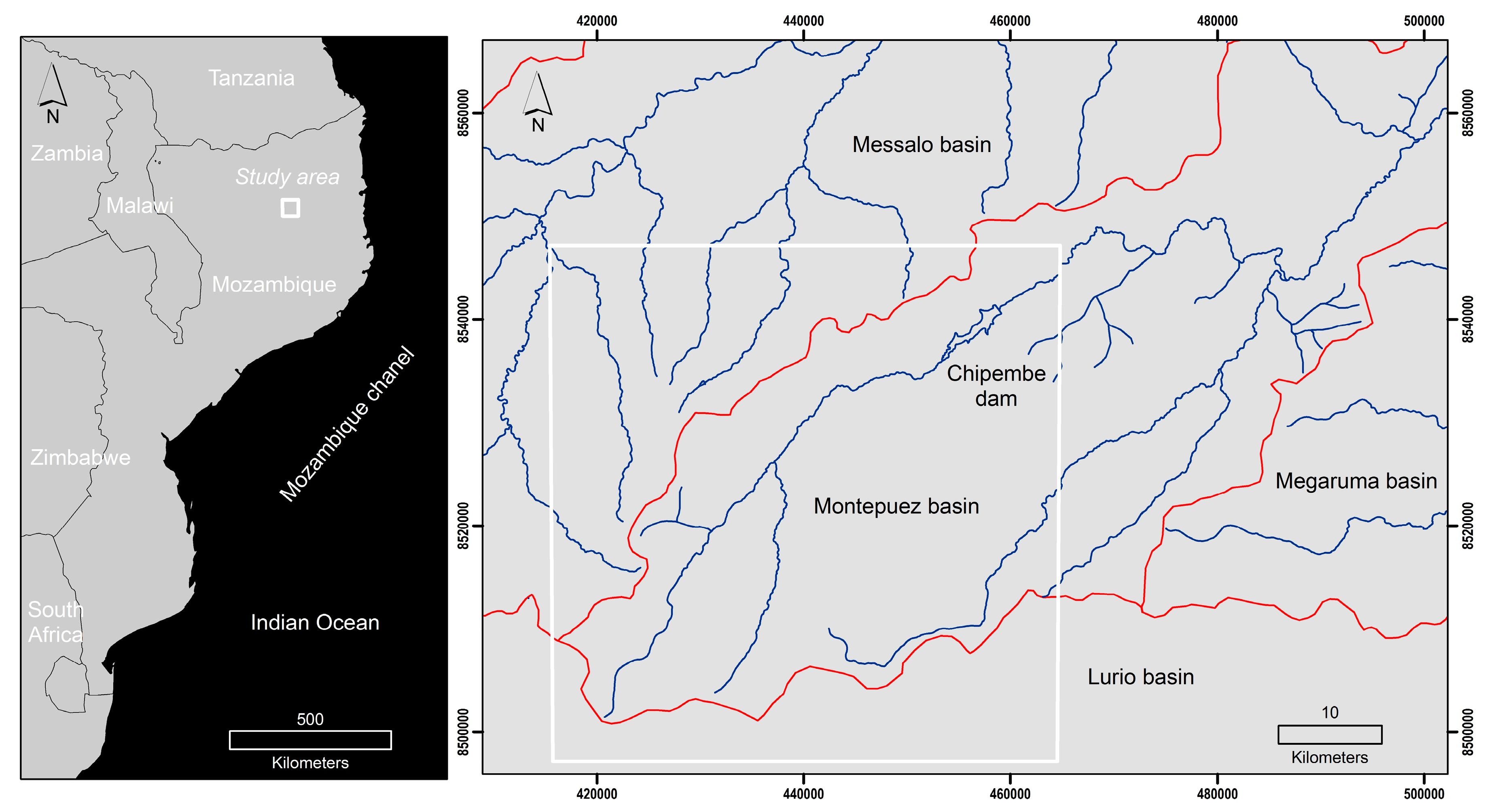
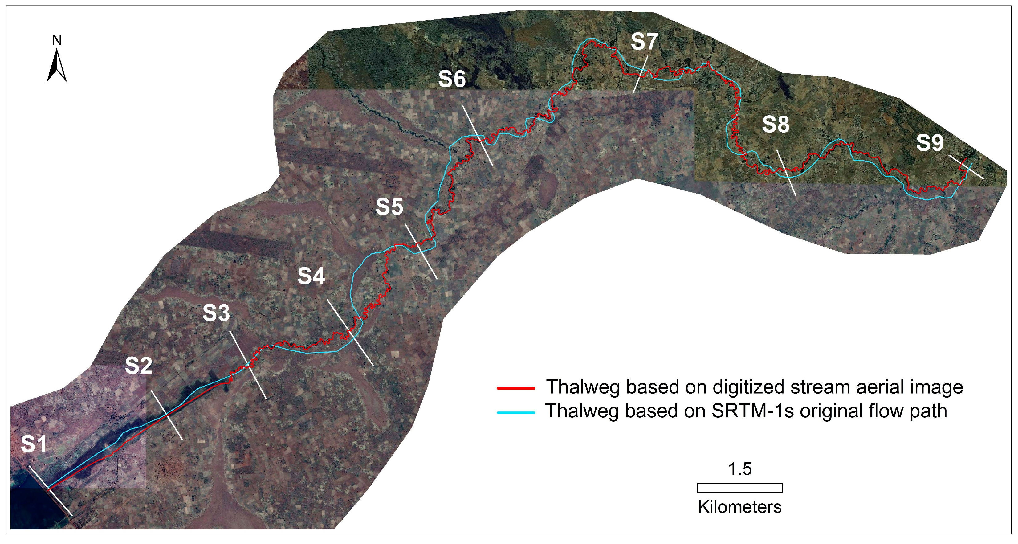
2. Study Site
3. Materials and Methods
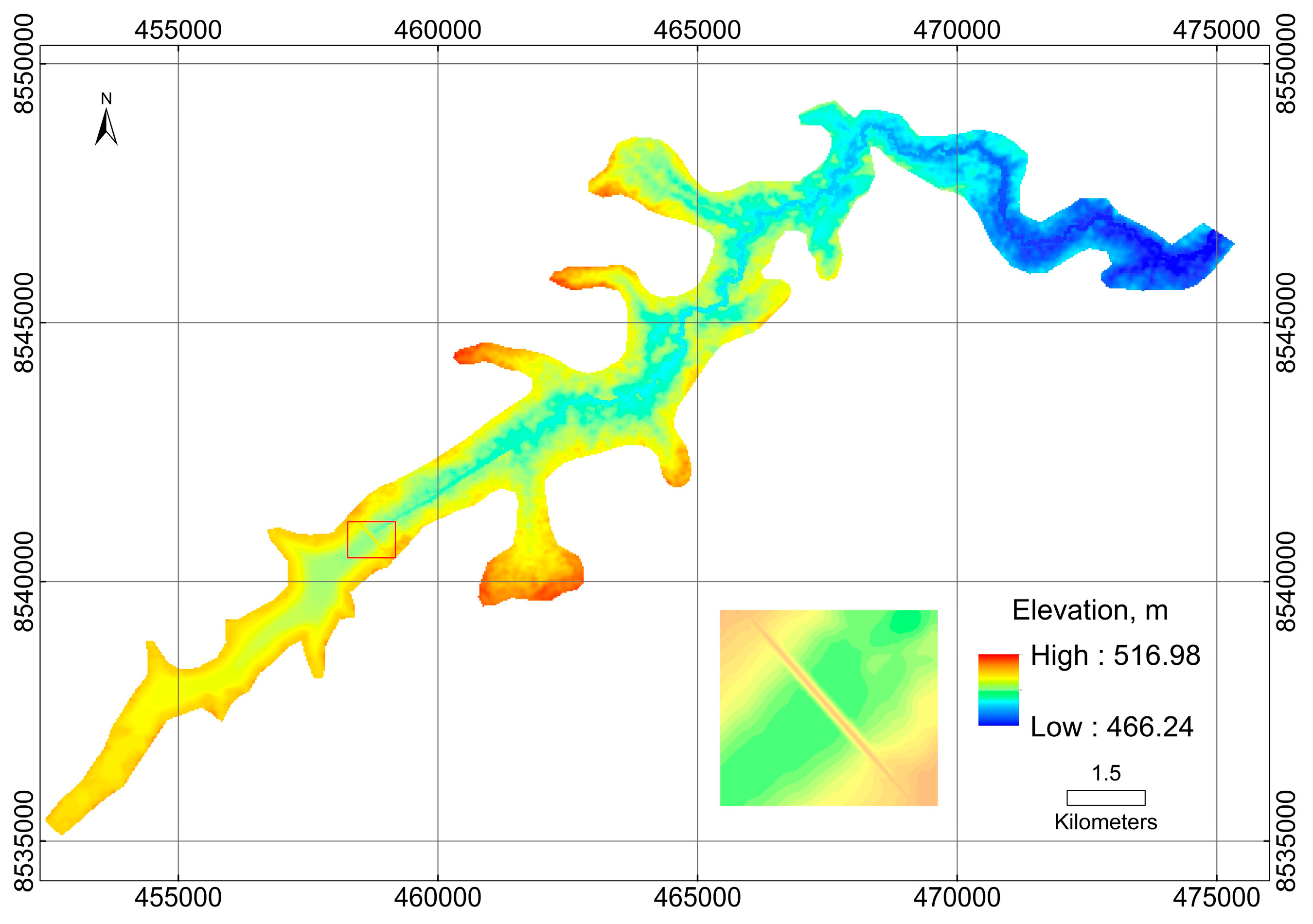
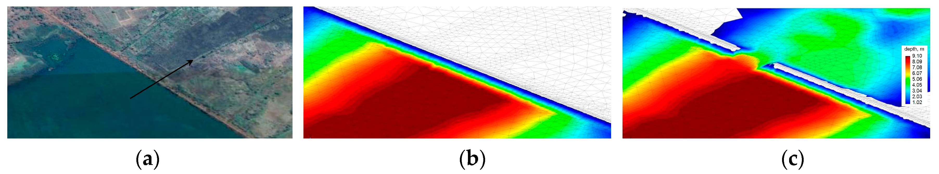
3.1. Cartographic Information
3.2. Hydraulic Model Description
3.3. Model Setup
4. Results and Discussion
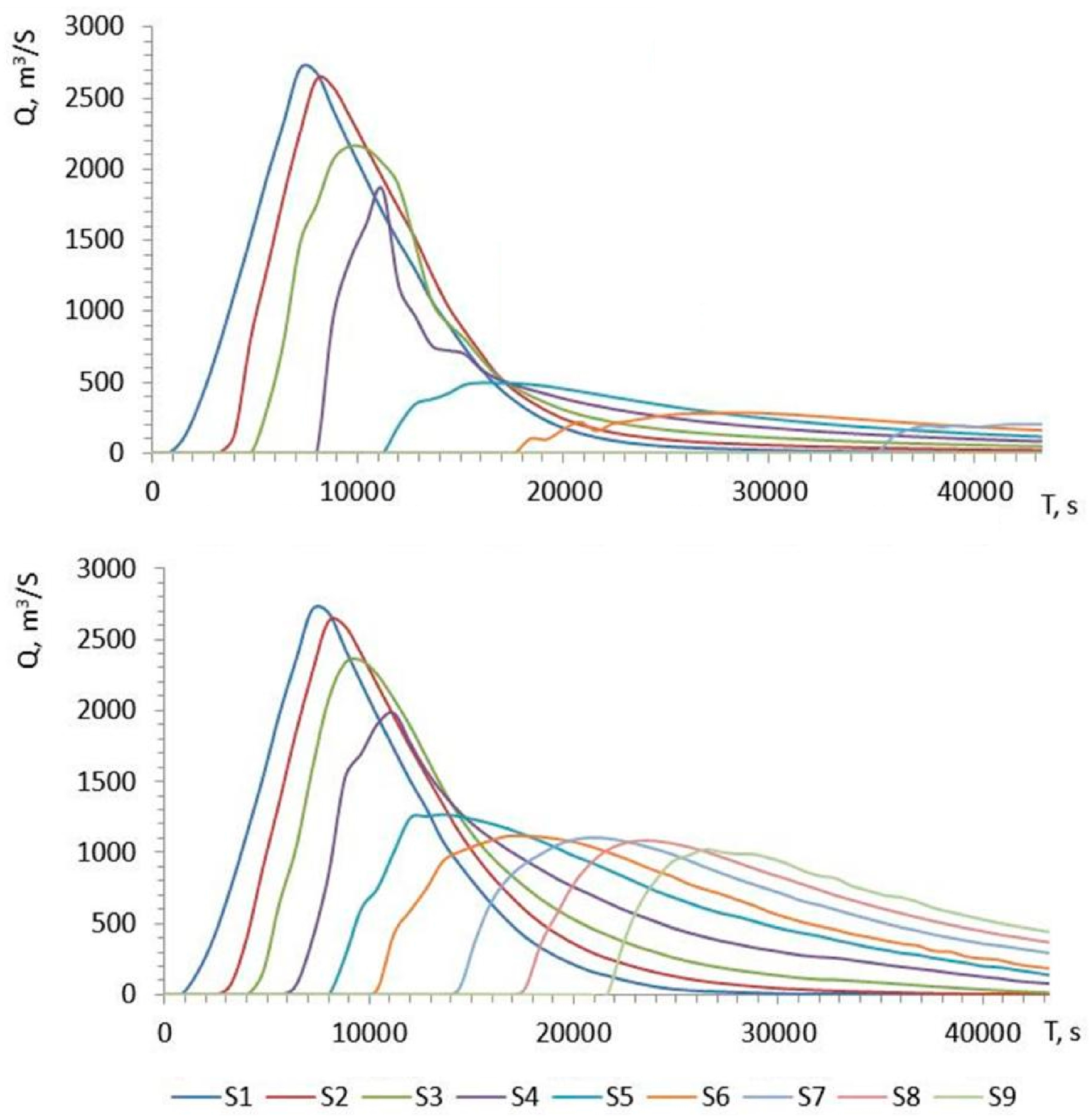
4.1. Peak Flows and Flood Wave Travel Times
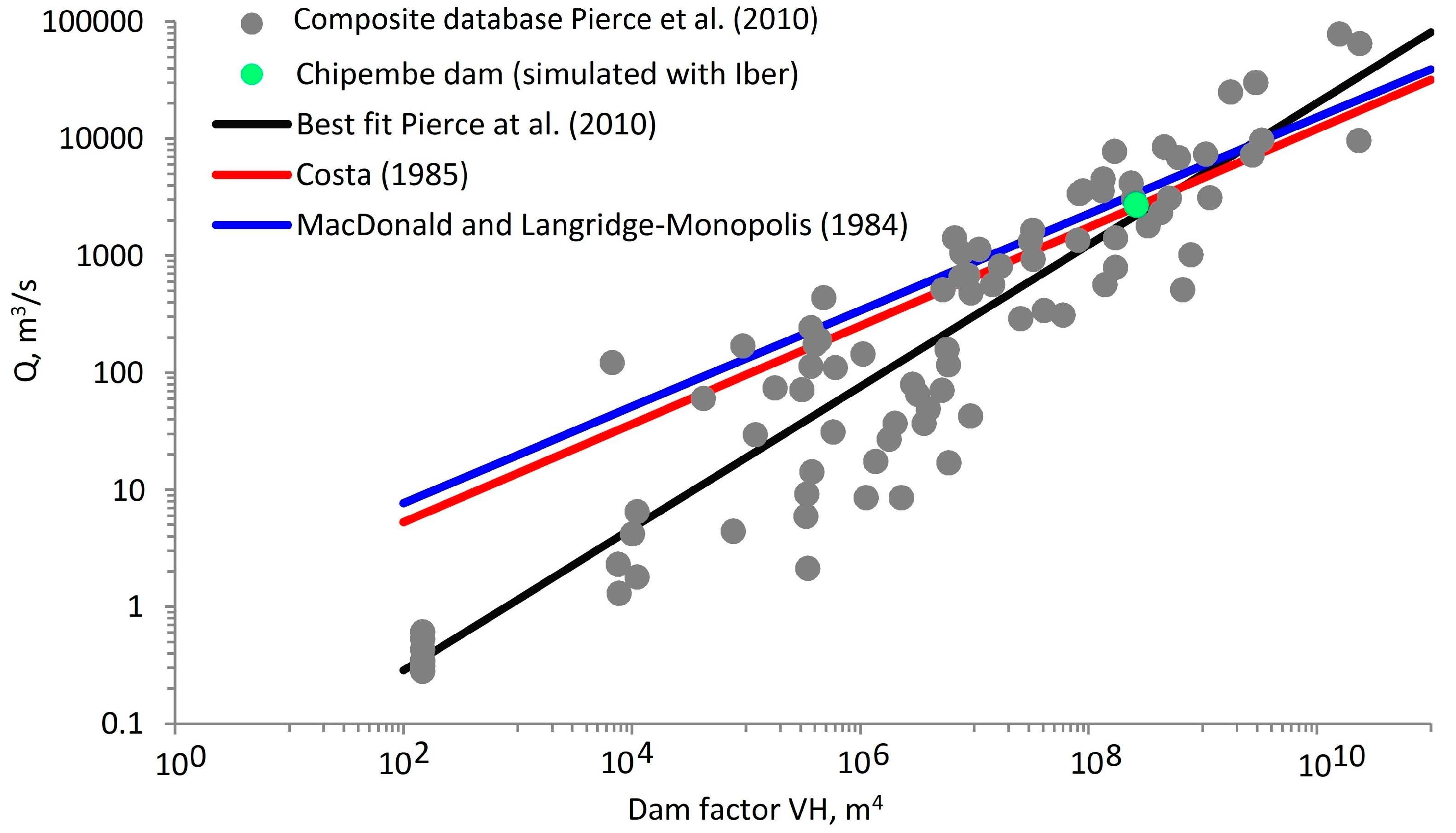
4.2. Comparison with Real Dam Failure Data
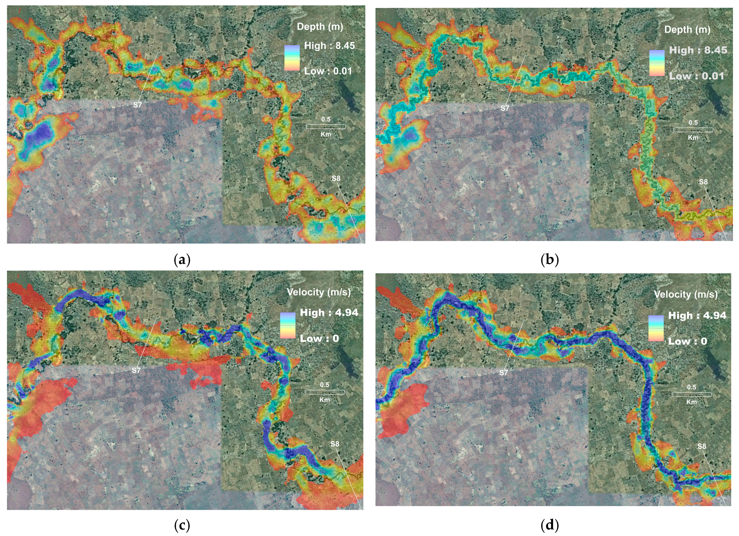
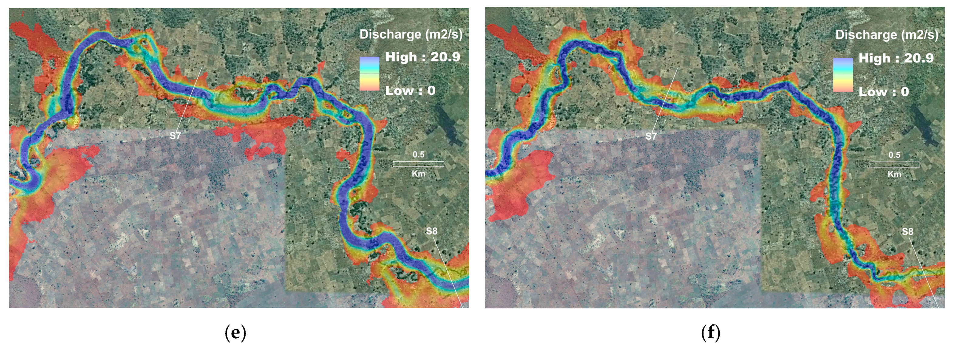
4.3. Flood Extent Delineation
4.4. Flood Hazard Mapping
4.5. Model Applicability
5. Conclusions
- (a)
- Higher peak discharges, up to ~10 times at the downstream section;
- (b)
- Lower peak flow attenuation, from ~90% to ~60% in the lower reach;
- (c)
- Lower time to peak and flood wave arrival time, reaching a 65% reduction at the downstream section;
- (d)
- Lower flood extent and flood width (~19%), and higher average flood depth (~9%).
Acknowledgments
Author Contributions
Conflicts of Interest
References
- Pilotti, M.; Maranzoni, M.; Tomirotti, M.; Valerio, G. 1923 Gleno dam break: Case study and numerical modeling. J. Hydraul. Eng. 2011, 137, 480–492. [Google Scholar] [CrossRef]
- Rogers, D.J. Lessons learned from the St. Francis Dam failure. Geo-Strata 2006, 6, 14–17. [Google Scholar]
- Jansen, R.B. Dam and Public Safety; US Department of the Interior, Water and Power Resources Service: Denver, CO, USA, 1980. [Google Scholar]
- Arthur, H.G. Teton Dam failure. The Evaluation of Dam Safety. In Proceedings of the Engineering Foundation Conference Proceedings, Pacific Grove, CA, USA, 28 November–3 December 1976; American Society of Civil Engineers: New York, NY, USA, 1977; pp. 61–71. [Google Scholar]
- Alcrudo, F.; Mulet, J. Description of the Tous Dam break case study (Spain). J. Hydraul. Res. 2007, 45, 45–57. [Google Scholar] [CrossRef]
- Menescal, R.A.; Vieira, V.P.; Oliveira, S.K. Terminologia para análise de risco e segurança de barragens. In A Segurança de Barragens E a Gestão de Recursos Hídricos; Menescal, R.A., Ed.; Ministério da Integração Nacional: Brasília, Brazil, 2005; pp. 31–39. (In Portuguese) [Google Scholar]
- Saxena, K.R.; Sharma, V.M. DAMS Incidents and Accidents; A.A. Balkema Publishers: Amsterdam, The Netherlands, 2005. [Google Scholar]
- U.S. Department of Interior Bureau of Reclamation (USBR). RCEM—Reclamation Consequence Estimating Methodology. Dam Failure and Flood Event Case History Compilation; U.S. Department of Interior Bureau of Reclamation: Washington, DC, USA, 2015.
- Gallegos, H.A.; Schubert, J.E.; Sanders, B.F. Structural damage prediction in a high-velocity urban dam-break flood: A field-scale assessment of predictive skill. J. Eng. Mech.-ASCE 2012, 138, 1249–1262. [Google Scholar] [CrossRef]
- Gee, D.M.; Brunner, G.W. Dam break flood routing using HEC-RAS and NWS-FLDWAV. In Impacts of Global Climate Change, Proceedings of the World Water and Environmental Resources Congress 2005, Anchorage, AK, USA, 15–19 May 2005; American Society of Civil Engineers: Reston, VA, USA, 2005; pp. 1–9. [Google Scholar] [CrossRef]
- Néelz, S.; Pender, G. Benchmarking the Latest Generation of 2D Hydraulic Modelling Packages; Report No. SC120002; Environment Agency: Bristol, UK, 2013. [Google Scholar]
- Soares-Frazão, S.; Canelas, R.; Cao, Z.; Cea, L.; Chaudhry, H.M.; Die Moran, A.; Kadi, K.E.; Ferreira, R.; Cadórniga, I.F.; Gonzalez-Ramirez, N.; et al. Dam-break flows over mobile beds: Experiments and benchmark tests for numerical models. J. Hydraul. Res. 2012, 50, 364–375. [Google Scholar] [CrossRef]
- Federal Emergency Management Agency. Federal Guidelines for Inundation Mapping of Flood Risks Associated with Dam Incidents and Failures; Federal Emergency Management Agency P-946; Federal Emergency Management Agency: Washington, DC, USA, 2013. [Google Scholar]
- Gallegos, H.A.; Schubert, J.E.; Sanders, B.F. Two-dimensional, high-resolution modeling of urban dam-break flooding: A case study of Baldwin Hills, California. Adv. Water Resour. 2009, 32, 1323–1335. [Google Scholar] [CrossRef]
- Horritt, M.S.; Bates, P.D. Effects of spatial resolution on a raster based model of flood flow. J. Hydrol. 2001, 253, 239–249. [Google Scholar] [CrossRef]
- Legleiter, C.J.; Roberts, D.A. A forward image model for passive optical remote sensing of river bathymetry. Remote Sens. Environ. 2009, 113, 1025–1045. [Google Scholar] [CrossRef]
- Trigg, M.A.; Wilson, M.D.; Bates, P.D.; Horrit, M.S.; Alsdorf, D.E.; Forsberg, B.R.; Vega, M.C. Amazon flood wave hydraulics. J. Hydrol. 2009, 374, 92–105. [Google Scholar] [CrossRef]
- Hodgson, M.E.; Jensen, J.R.; Schmidt, L.; Schill, S.; Davis, B. An evaluation of LIDAR- and IFSAR-derived digital elevation models in leaf-on conditions with USGS Level 1 and Level 2 DEMs. Remote Sens. Environ. 2003, 84, 295–308. [Google Scholar] [CrossRef]
- Smith, M.J.; Edwards, E.P.; Priestnall, G.; Bates, P.D. Exploitation of New Data Types to Create Digital Surface Models for flood Inundation Modeling; FRMRC Research Report UR3; FRMRC: University of Manchester, Manchester, UK, 2006. [Google Scholar]
- Bates, P.D.; Marks, K.J.; Horritt, M.S. Optimal use of high-resolution topographic data in flood inundation models. Hydrol. Process. 2003, 17, 537–557. [Google Scholar] [CrossRef]
- Cobby, D.M.; Mason, D.C.; Horritt, M.S.; Bates, P.D. Two-dimensional hydraulic flood modelling using a finite-element mesh decomposed according to vegetation and topographic features derived from airborne scanning laser altimetry. Hydrol. Process. 2003, 17, 1979–2000. [Google Scholar] [CrossRef]
- Sanders, B.F. Evaluation of on-line DEMs for flood inundation modeling. Adv. Water Resour. 2007, 30, 1831–1843. [Google Scholar] [CrossRef]
- Rabus, B.; Eineder, M.; Roth, A.; Bamler, R. The shuttle radar topography mission—A new class of digital elevation models acquired by spaceborne radar. ISPRS J. Photogramm. Remote Sens. 2003, 57, 241–262. [Google Scholar] [CrossRef]
- Van Zyl, J.J. The shuttle radar topography mission (SRTM): A breakthrough in remote sensing of topography. Acta Astronaut. 2001, 48, 559–565. [Google Scholar] [CrossRef]
- Sampson, C.C.; Smith, A.; Bates, P.D.; Neal, J.C.; Trigg, M.A. Perspectives on open access high resolution digital elevation models to produce global flood hazard layers. Front. Earth Sci. 2016, 3, 1–6. [Google Scholar] [CrossRef]
- Bladé, E.; Cea, L.; Corestein, G.; Escolano, E.; Puertas, J.; Vázquez-Cendón, E.; Dolz, J.; Coll, A. Iber: Herramienta de simulación numérica del flujo en ríos. Iber—River modelling simulation tool. Rev. Int. Métodos Numér. Para Cálc. Diseño Ing. 2014, 30, 1–10. (In Spanish) [Google Scholar] [CrossRef]
- Pierce, M.W.; Thornton, C.I.; Abt, S.R. Predicting peak outflow from breached embankment dams. J. Hydraul. Eng. 2010, 15, 338–349. [Google Scholar] [CrossRef]
- Universidade da Coruña. Manual Técnico de Planificação e Gestão de Infraestructuras Hidráulicas das Bacias Internas de Cabo Delgado; Technical Manual for Planning and Management of Hydraulic Infrastructures in the Interior Catchments of Cabo Delgado; Internal Report; Universidade da Coruña: A Coruña, España, 2014. (In Portuguese) [Google Scholar]
- Jones, A.; Breuning-Madsen, H.; Brossard, M.; Dampha, A.; Deckers, J.; Dewitte, O.; Gallali, T.; Hallett, S.; Jones, R.; Kilasara, M.; et al. Soil Atlas of Africa; European Commission, Publications Office of the European Union: Luxembourg, 2013. [Google Scholar]
- EIA—Avaliação de Impacto Ambiental. Reabilitação da Barragem de Chipembe: Instrução do Processo; Estudo do Impacto Sócio—Ambiental: Pemba, Mozambique, 2013. (In Portuguese) [Google Scholar]
- Farr, T.G.; Rosen, P.A.; Caro, E.; Crippen, R.; Duren, R.; Hensley, S.; Kobrick, M.; Paller, M.; Rodriguez, E.; Roth, L.; et al. The shuttle radar topography mission. Rev. Geophys. 2007, 45, 1–43. [Google Scholar] [CrossRef]
- Yan, K.; Di Baldassarre, G.; Solomatine, D.P.; Schumann, G.J.P. A review of low-cost space-borne data for flood modelling: Topography, flood extent and water level. Hydrol. Process. 2015, 29, 3368–3387. [Google Scholar] [CrossRef]
- Kreiselmeier, J. Development of a Flood Model Based on Globally-Available Satellite Data for the Papaloapan River, Mexico, 2015. (Dissertation). Available online: http://urn.kb.se/resolve?urn=urn:nbn:se:uu:diva-256399 (accessed on 9 June 2017).
- Simard, M.; Pinto, N.; Fisher, J.B.; Baccini, A. Mapping forest canopy height globally with spaceborne lidar. J. Geophys. Res. Biogeosci. 2011, 116, G04021. [Google Scholar] [CrossRef]
- Callow, J.N.; van Niel, K.P.; Boggs, G.S. How does modifying a DEM to reflect known hydrology affect subsequent terrain analysis. J. Hydrol. 2007, 332, 30–39. [Google Scholar] [CrossRef]
- Lindsay, J. The practice of DEM stream burning revisited. Earth Surf. Process. Landf. 2016, 41, 658–668. [Google Scholar] [CrossRef]
- Neal, J.C.; Odoni, N.A.; Trigg, M.A.; Freer, J.E.; Garcia-Pintado, J.; Mason, D.C.; Wood, M.; Bates, P.D. Efficient incorporation of channel cross-section geometry uncertainty into regional and global scale flood inundation models. J. Hydrol. 2015, 529, 169–183. [Google Scholar] [CrossRef]
- Morris, M.W. Concerted Action on Dambreak Modelling—CADAM; Final Report SR 571; HR Wallingford Ltd.: Wallingford, UK, 2000. [Google Scholar]
- Bladé, E.; Cea, L.; Corestein, C. Modelización numérica de inundaciones fluviales. Ing. Agua 2014, 18, 71–81. [Google Scholar] [CrossRef]
- Cea, L.; Bermudez, M.; Puertas, J.; Blade, E.; Corestein, G.; Escolano, E.; Conde, A.; Bockelmann-Evans, B.; Ahmadian, R. IberWQ: New simulation tool for 2D water quality modelling in rivers and shallow estuaries. J. Hydroinform. 2016, 18, 816–830. [Google Scholar] [CrossRef]
- González-Aguirre, J.; Vázquez-Cendón, M.E.; Alavez-Ramírez, J. Simulación numérica de inundaciones en Villahermosa México usando el código Iber (Flood modelling in Villahermosa Mexico with the model Iber). Ing. Agua 2016, 20, 201–218. [Google Scholar] [CrossRef]
- Castillo, L.; Carrillo, J.; Álvarez, M. Complementary Methods for Determining the Sedimentation and Flushing in a Reservoir. J. Hydraul. Eng. 2015, 141, 5015004. [Google Scholar] [CrossRef]
- Castillo, C.; Pérez, R.; Gómez, J. A conceptual model of check dam hydraulics for gully control: Efficiency, optimal spacing and relation with step-pools. Hydrol. Earth Syst. Sci. 2014, 18, 1705–1721. [Google Scholar] [CrossRef]
- Cannata, M.; Marzocchi, R. Two-dimensional dam break flooding simulation: A GIS-embedded approach. Nat. Hazards 2012, 61, 1143–1159. [Google Scholar] [CrossRef]
- Wang, L.; Liang, Q.; Kesserwani, G.; Hall, J. A 2D shallow flow model for practical dam-break simulations. J. Hydraul. Res. 2011, 49, 307–316. [Google Scholar] [CrossRef]
- Roe, P.L. Discrete models for the numerical analysis of time-dependent multi-dimensional gas dynamics. J. Comput. Phys. 1986, 63, 458–476. [Google Scholar] [CrossRef]
- Bermúdez, A.; Dervieux, A.; Desideri, J.A.; Vázquez, M.E. Upwind schemes for the two-dimensional shallow water equations with variable depth using unstructured meshes. Comput. Methods Appl. Mech. Eng. 1998, 155, 49–72. [Google Scholar] [CrossRef]
- Cea, L.; Puertas, J.; Vázquez-Cendón, M.E. Depth averaged modelling of turbulent shallow water flow with wet-dry fronts. Arch. Comput. Methods Eng. State Art Rev. 2007, 3, 303–341. [Google Scholar] [CrossRef]
- Rastogi, A.K.; Rodi, W. Predictions of heat and mass transfer in open channels. J. Hydraul. Div. 1978, 104, 397–420. [Google Scholar]
- Wahl, T.L.; Hanson, G.J.; Courivaud, J.; Morris, M.W.; Kahawita, R.; McClenathan, J.T.; Gee, D.M. Development of next-generation embankment dam breach models. In Proceedings of the US Society of Dams Annual Meeting and Conference 2008, Portland, OR, USA, 28 April–2 May 2008. [Google Scholar]
- Ministerio del Medio Ambiente. Clasificación de Presas en Función del Riesgo Potencial (Guidelines for Dam Classification According to their Potential Risk of Failure); Dirección General de Obras Hidráulicas y Calidad de las Aguas: Madrid, Spain, 1996; p. 64. (In Spanish)
- Wahl, T.L. Uncertainty of predictions of embankment dam breach parameters. J. Hydraul. Eng. 2004, 130, 389–397. [Google Scholar] [CrossRef]
- Wu, W.; Altinakar, M.S.; Bradford, S.F.; Chen, Q.J.; Constantinescu, S.G.; Duan, J.G.; Gee, D.M.; Greimann, B.; Hanson, G.; Zhiguo, H.; et al. Earthen embankment breaching. J. Hydraul. Eng. 2011, 137, 1549–1564. [Google Scholar] [CrossRef]
- Jonkman, S.N.; Vrijling, J.K.; Vrouwenvelder, A.C.W.M. Methods for the estimation of loss of life due to floods: A literature review and a proposal for a new method. Nat. Hazards 2008, 46, 353–389. [Google Scholar] [CrossRef]
- International Committee on Large Dams (ICOLD). Small Dams Design, Surveillance and Rehabilitation; International Committee on Large Dams: Paris, France, 2011; p. 159. [Google Scholar]
- Evans, S.G. The maximum discharge of outburst floods caused by the breaching of man-made and natural dams. Can. Geotech. J. 1986, 23, 385–387. [Google Scholar] [CrossRef]
- Singh, K.P.; Snorrason, A. Sensitivity of outflow peaks and flood stages to the selection of dam breach parameters and simulation models. J. Hydrol. 1984, 68, 295–310. [Google Scholar] [CrossRef]
- MacDonald, T.; Langridge-Monopolis, J. Breaching charateristics of dam failures. J. Hydraul. Eng. 1984, 110, 567–586. [Google Scholar] [CrossRef]
- Costa, J.E. Floods from Dam Failures; Open File Report 85-560; US Geological Survey: Denver, CO, USA, 1985; p. 54.
- Yan, K.; Neal, J.C.; Solomatine, D.P.; Di Baldassarre, G. Global and low-cost topographic data to support flood studies. In Hydro-Meteorological Hazards, Risks, and Disaster, 1st ed.; Shroder, J.F., Paron, P., Di Baldassarre, G., Eds.; Elsevier: Amsterdam, The Netherlands, 2014; pp. 105–124. [Google Scholar]


| Section | L (km) | Qp (m3/s) | Ta (h) | Tp (h) | Qp (m3/s) | Ta (h) | Tp (h) | Qp (m3/s) | Ta (h) | Tp (h) |
|---|---|---|---|---|---|---|---|---|---|---|
| n = 0.02 m−1/3·s | n = 0.03 m−1/3·s | n = 0.04 m−1/3·s | ||||||||
| S1 | 0.1 | 2747.6 | - | 2 | 2702.9 | - | 2.0 | 2673.9 | - | 2.0 |
| S2 | 2.5 | 2716.8 | 0.9 | 2.2 | 2637.3 | 1.1 | 2.2 | 2527.7 | 1.1 | 2.2 |
| S3 | 4.6 | 2271.8 | 1.3 | 2.7 | 2160.1 | 1.3 | 2.7 | 2053.1 | 1.6 | 2.9 |
| S4 | 8.3 | 1901.5 | 2.0 | 2.9 | 1863.7 | 2.0 | 3.1 | 1711.2 | 2.2 | 3.3 |
| S5 | 12.3 | 546.6 | 2.9 | 4.2 | 497.4 | 3.1 | 4.4 | 442.4 | 3.1 | 4.7 |
| S6 | 16.4 | 326.3 | 4.7 | 7.3 | 287.1 | 4.9 | 7.8 | 253.1 | 5.3 | 8.7 |
| S7 | 22.8 | 232.9 | 8.9 | 10.7 | 204.3 | 9.8 | 11.8 | 181.1 | 10.7 | 13.1 |
| S8 | 30.3 | 162.6 | 11.8 | 14.4 | 143.4 | 12.9 | 15.8 | 125.8 | 14.2 | 17.3 |
| S9 | 35.9 | 109.3 | 16.0 | 18.2 | 95.5 | 17.6 | 20.0 | 84.1 | 19.6 | 22.4 |
| n = 0.05 m−1/3·s | n = 0.06 m−1/3·s | - | ||||||||
| S1 | 0.1 | 2619.8 | - | 2.0 | 2556.4 | - | 2.0 | - | - | - |
| S2 | 2.5 | 2451.3 | 1.1 | 2.2 | 2350.9 | 1.1 | 2.2 | - | - | - |
| S3 | 4.6 | 1938.8 | 1.6 | 2.9 | 1801.8 | 1.6 | 3.1 | - | - | - |
| S4 | 8.3 | 1557.9 | 2.4 | 3.3 | 1449.5 | 2.4 | 3.6 | - | - | - |
| S5 | 12.3 | 390.5 | 3.3 | 5.1 | 346.6 | 3.6 | 5.3 | - | - | - |
| S6 | 16.4 | 221.6 | 5.8 | 9.6 | 195.3 | 6.2 | 10.7 | - | - | - |
| S7 | 22.8 | 160.2 | 11.8 | 14.2 | 141.6 | 13.1 | 15.8 | - | - | - |
| S8 | 30.3 | 111.6 | 15.8 | 19.8 | 99.1 | 17.6 | 21.6 | - | - | - |
| S9 | 35.9 | 76.2 | 21.8 | 25.1 | 66.0 | 24.2 | 27.8 | - | - | - |
| Section | L (km) | Qp (m3/s) | Ta (h) | Tp (h) | Qp (m3/s) | Ta (h) | Tp (h) | Qp (m3/s) | Ta (h) | Tp (h) |
|---|---|---|---|---|---|---|---|---|---|---|
| n = 0.02 m−1/3·s | n = 0.03 m−1/3·s | n = 0.04 m−1/3·s | ||||||||
| S1 | 0.1 | 2746.5 | - | 2.0 | 2710.0 | - | 2.0 | 2664.5 | - | 2.0 |
| S2 | 2.5 | 2722.9 | 0.7 | 2.2 | 2629.5 | 0.7 | 2.2 | 2523.1 | 0.89 | 2.4 |
| S3 | 4.6 | 2450.4 | 1.1 | 2.4 | 2354.0 | 1.1 | 2.7 | 2240.8 | 1.33 | 2.7 |
| S4 | 8.3 | 2094.1 | 1.6 | 2.9 | 1981.9 | 1.6 | 3.1 | 1831.2 | 1.78 | 3.1 |
| S5 | 12.3 | 1376.1 | 2.0 | 3.5 | 1268.9 | 2.2 | 3.8 | 1162.3 | 2.44 | 3.8 |
| S6 | 16.4 | 1185.4 | 2.7 | 4.7 | 1117.8 | 2.7 | 4.7 | 1027.1 | 2.89 | 4.9 |
| S7 | 22.8 | 1181.0 | 3.6 | 5.8 | 1104.8 | 3.8 | 5.8 | 1002.5 | 4.22 | 6.2 |
| S8 | 30.3 | 1159.9 | 4.4 | 6.2 | 1083.6 | 4.7 | 6.4 | 978.1 | 5.11 | 7.1 |
| S9 | 35.9 | 1106.7 | 5.6 | 7.1 | 1021.0 | 6.0 | 7.3 | 901.0 | 6.44 | 8.0 |
| n = 0.05 m−1/3·s | n = 0.06 m−1/3·s | - | ||||||||
| S1 | 0.1 | 2587.1 | - | 2.0 | 2532.9 | - | 2.0 | - | - | - |
| S2 | 2.5 | 2441.8 | 0.9 | 2.4 | 2348.5 | 0.9 | 2.4 | - | - | - |
| S3 | 4.6 | 2115.9 | 1.3 | 2.7 | 2005.5 | 1.6 | 2.9 | - | - | - |
| S4 | 8.3 | 1723.5 | 1.8 | 3.3 | 1605.7 | 2.0 | 3.6 | - | - | - |
| S5 | 12.3 | 1076.1 | 2.4 | 4.0 | 990.1 | 2.7 | 4.4 | - | - | - |
| S6 | 16.4 | 939.9 | 3.1 | 5.3 | 855.1 | 3.3 | 5.6 | - | - | - |
| S7 | 22.8 | 911.3 | 4.4 | 6.7 | 827.7 | 4.9 | 7.1 | - | - | - |
| S8 | 30.3 | 885.4 | 5.6 | 7.6 | 801.9 | 6.0 | 8.0 | - | - | - |
| S9 | 35.9 | 824.2 | 6.9 | 8.9 | 739.6 | 7.6 | 9.8 | - | - | - |
| n (m−1/3·s) | Flooded Area (×106 m2) | Average Flood Depth (m) | Maximum Depth (m) | Average Flood Width (m) | ||||
|---|---|---|---|---|---|---|---|---|
| A | B | A | B | A | B | A | B | |
| 0.02 | 13.28 | 10.98 | 2.72 | 2.94 | 9.58 | 8.67 | 368 | 305 |
| 0.03 | 13.30 | 11.06 | 2.75 | 3.02 | 9.61 | 8.69 | 369 | 307 |
| 0.04 | 13.34 | 11.22 | 2.78 | 3.06 | 9.61 | 8.73 | 370 | 312 |
| 0.05 | 13.39 | 11.35 | 2.80 | 3.12 | 9.62 | 8.76 | 372 | 315 |
| 0.06 | 13.45 | 11.49 | 2.82 | 3.15 | 9.62 | 8.77 | 373 | 319 |
© 2017 by the authors. Licensee MDPI, Basel, Switzerland. This article is an open access article distributed under the terms and conditions of the Creative Commons Attribution (CC BY) license (http://creativecommons.org/licenses/by/4.0/).
Share and Cite
Álvarez, M.; Puertas, J.; Peña, E.; Bermúdez, M. Two-Dimensional Dam-Break Flood Analysis in Data-Scarce Regions: The Case Study of Chipembe Dam, Mozambique. Water 2017, 9, 432. https://doi.org/10.3390/w9060432
Álvarez M, Puertas J, Peña E, Bermúdez M. Two-Dimensional Dam-Break Flood Analysis in Data-Scarce Regions: The Case Study of Chipembe Dam, Mozambique. Water. 2017; 9(6):432. https://doi.org/10.3390/w9060432
Chicago/Turabian StyleÁlvarez, Manuel, Jerónimo Puertas, Enrique Peña, and María Bermúdez. 2017. "Two-Dimensional Dam-Break Flood Analysis in Data-Scarce Regions: The Case Study of Chipembe Dam, Mozambique" Water 9, no. 6: 432. https://doi.org/10.3390/w9060432
APA StyleÁlvarez, M., Puertas, J., Peña, E., & Bermúdez, M. (2017). Two-Dimensional Dam-Break Flood Analysis in Data-Scarce Regions: The Case Study of Chipembe Dam, Mozambique. Water, 9(6), 432. https://doi.org/10.3390/w9060432