
Evaluation of Spatio-Temporal Patterns of Remotely Sensed Evapotranspiration to Infer Information about Hydrological Behaviour in a Data-Scarce Region


Abstract
:1. Introduction
2. Material and Methods
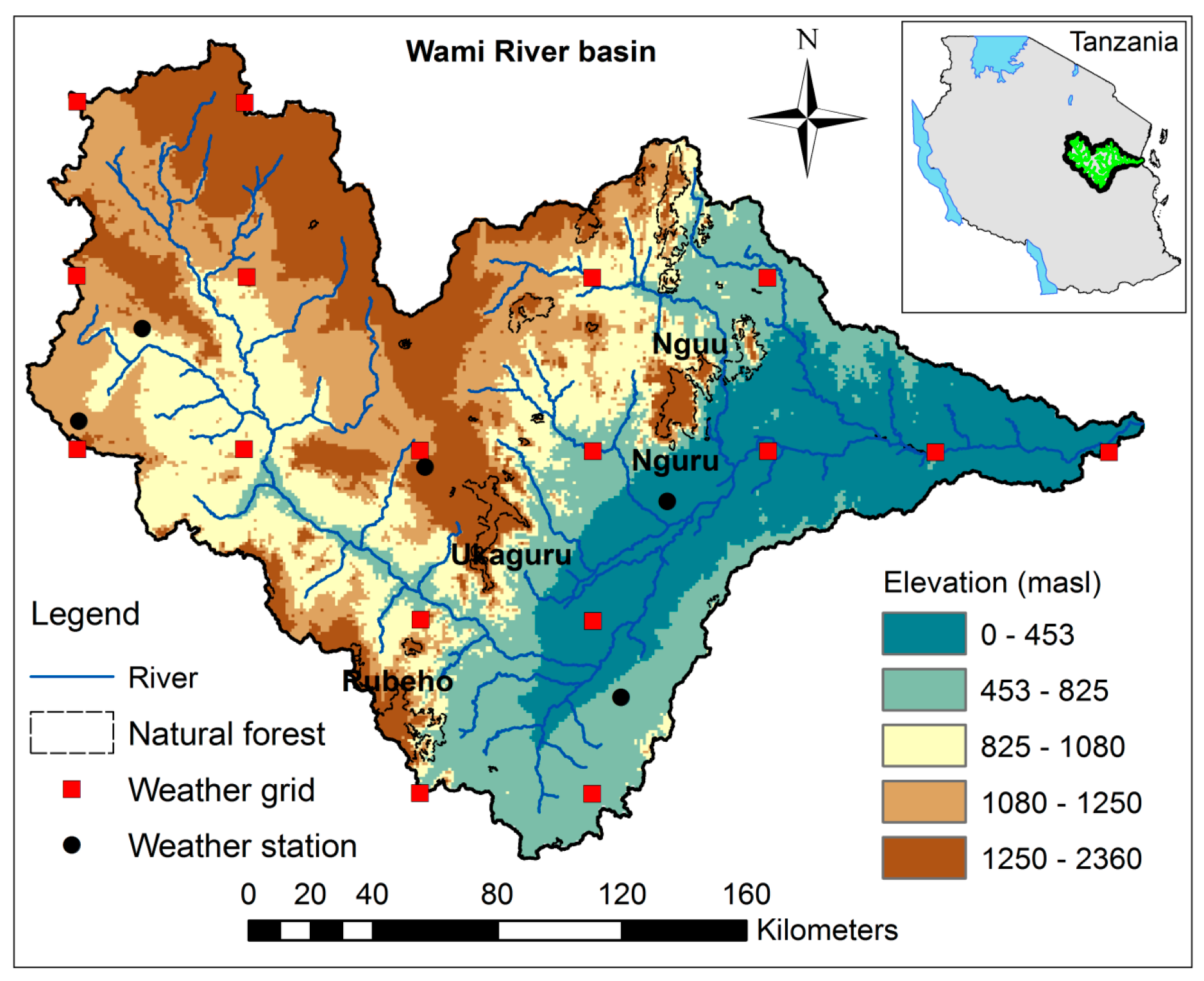
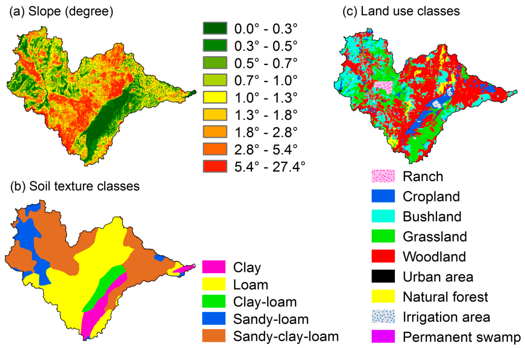
2.1. Study Area
2.2. Data
2.2.1. Land Surface and Meteorological Data
2.2.2. MODIS ET Data and Pre-Processing
2.3. Analysis of Hydrological Behaviour
2.3.1. Principal Component Analysis
2.3.2. Trend Tests
2.4. Land Surface Drivers of Hydrological Behaviour
2.4.1. Statistical Dependence Test for Metric Data
2.4.2. Statistical Difference Test for Nominal Data
3. Results
3.1. Trends in Meteorological Data
3.2. Principal Components
3.2.1. First Principal Component
3.2.2. Second Principal Component
3.2.3. Third Principal Component
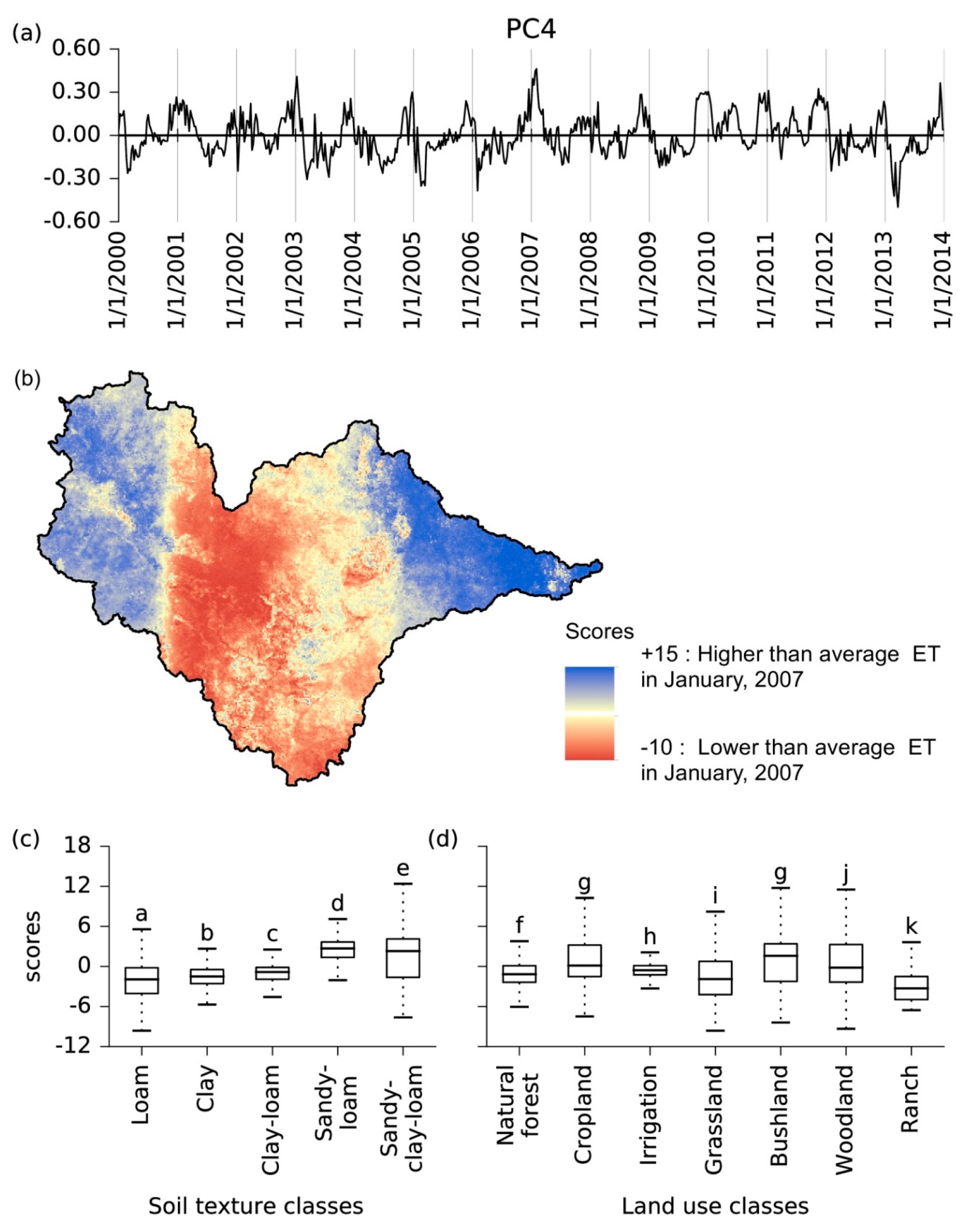
3.2.4. Fourth Principal Component
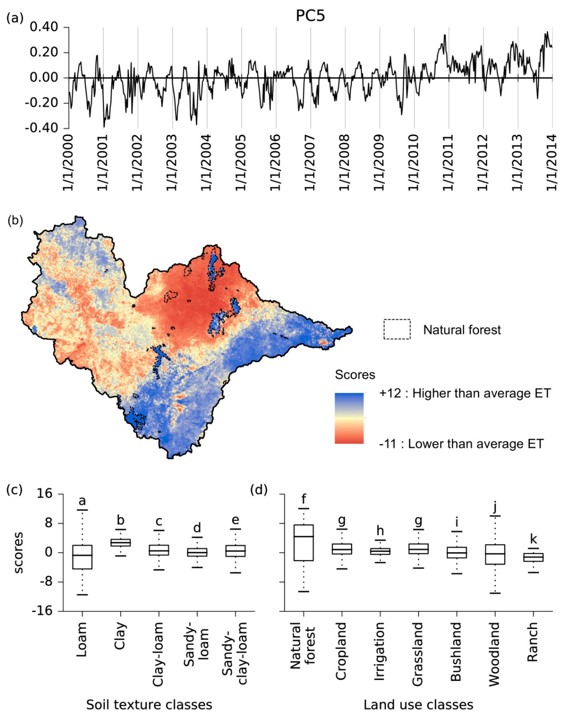
3.2.5. Fifth Principal Component
4. Discussion
4.1. General Approach
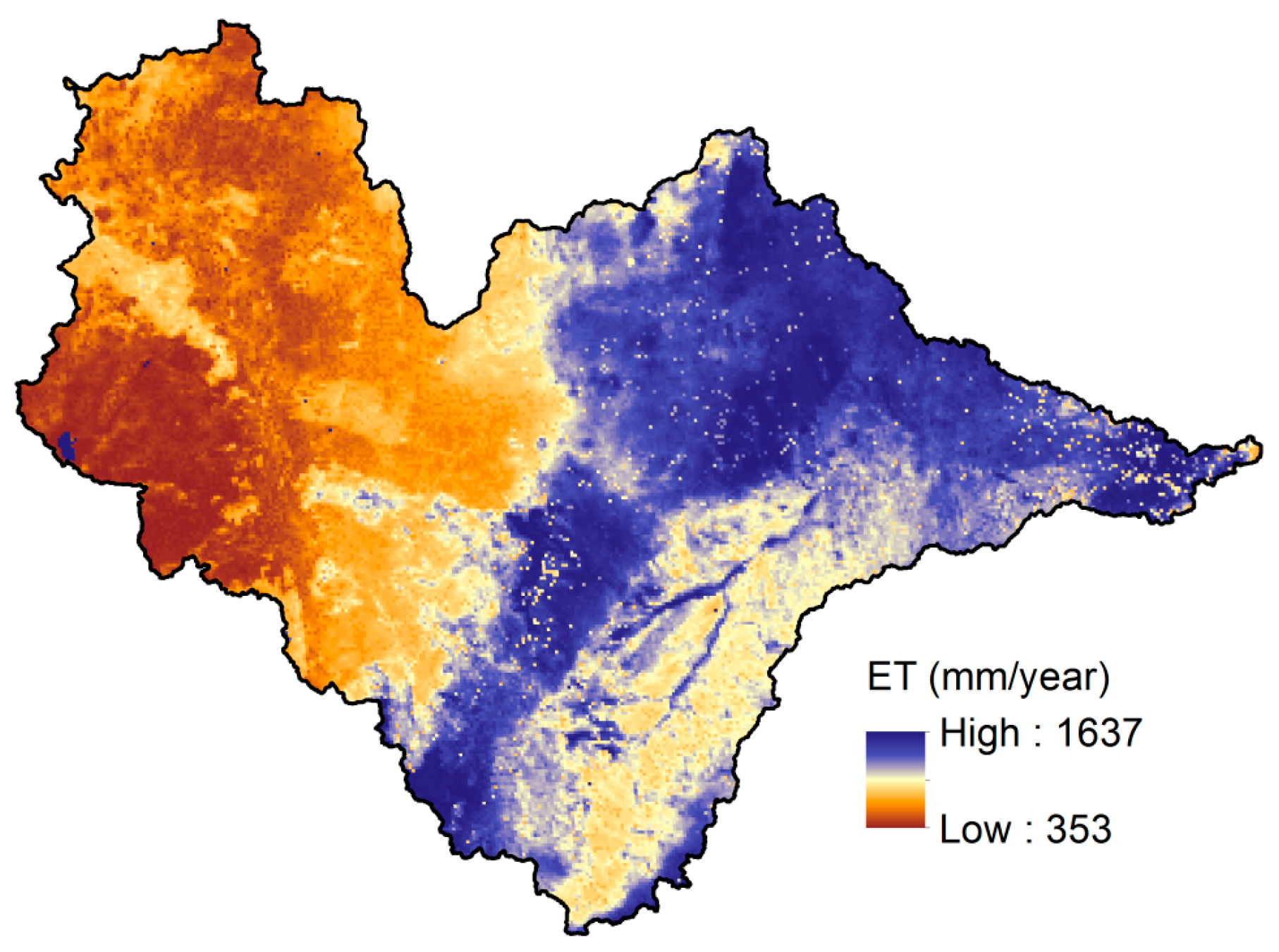
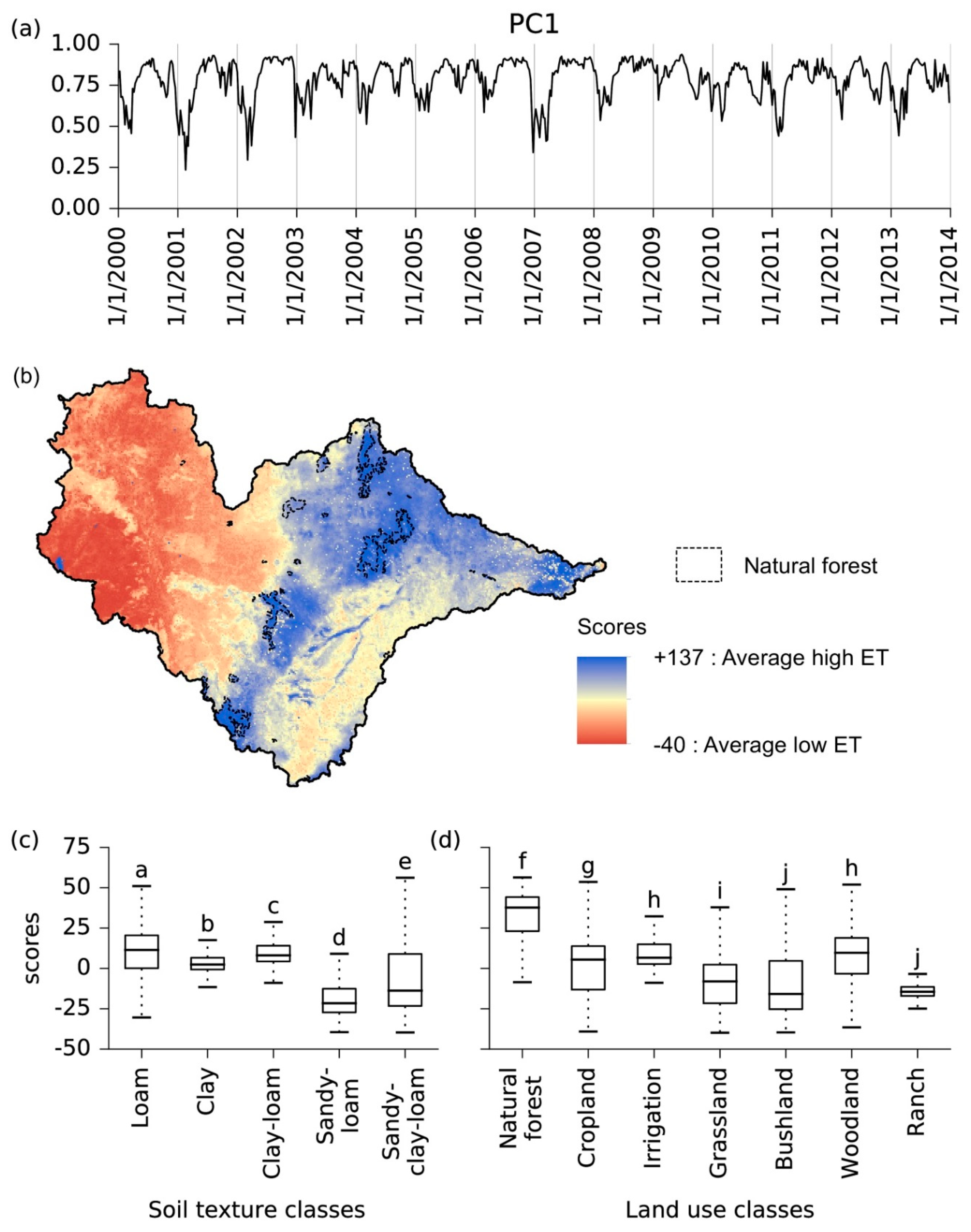
4.2. First Principal Component: Mean Behaviour of ET
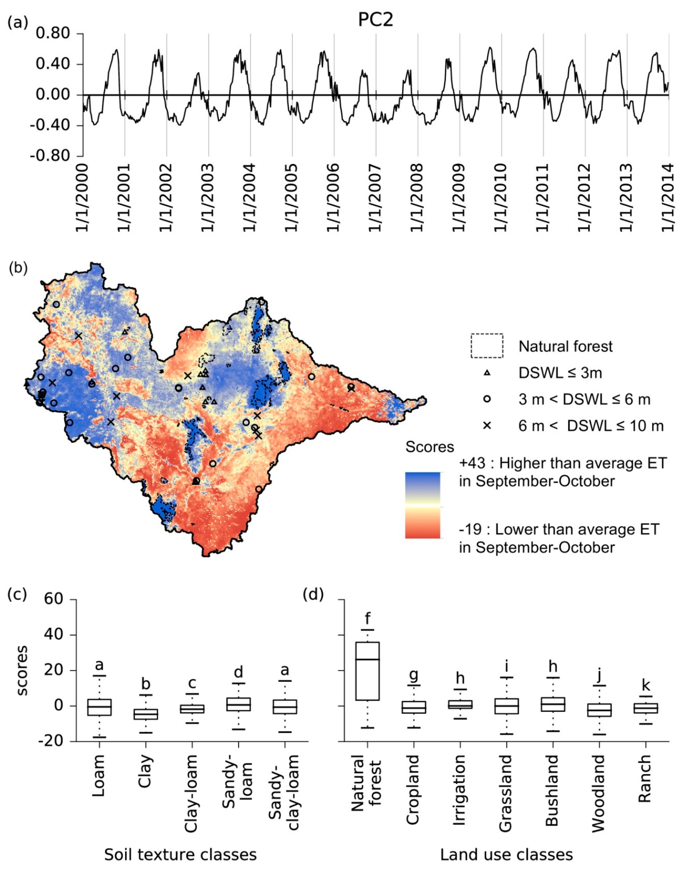
4.3. Second Principal Component: Dry Season Effects
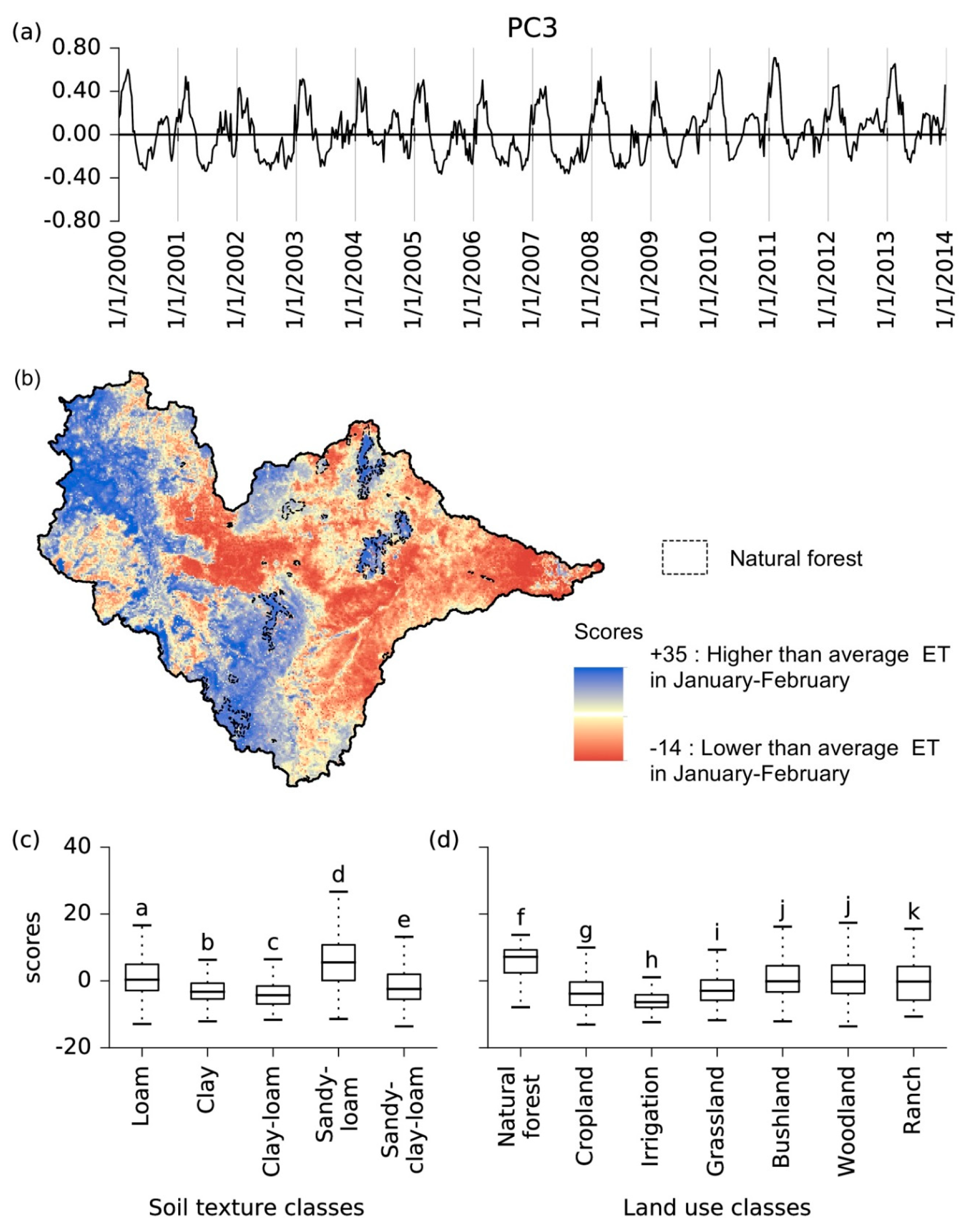
4.4. Third Principal Component: General Spatial Patterns of Rainfall
4.5. Fourth Principal Component: Single Major Rainstorms
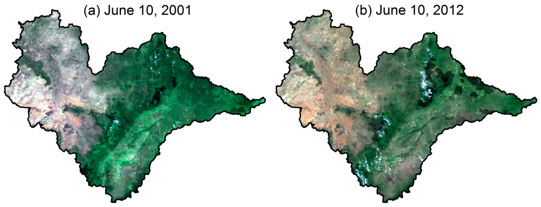
4.6. Fifth Principal Component: Long-Term Trend of Land Use
4.7. Implications for Water Resources Management and Distributed Hydrological Models
5. Conclusions
Supplementary Materialss
Acknowledgment
Author Contributions
Conflicts of Interest
References
- Li, Z.-L.; Tang, R.; Wan, Z.; Bi, Y.; Zhou, C.; Tang, B.; Yan, G.; Zhang, X. A review of current methodologies for regional evapotranspiration estimation from remotely sensed data. Sensors 2009, 9, 3801–3853. [Google Scholar] [CrossRef] [PubMed]
- Eswar, R.; Sekhar, M.; Bhattacharya, B.K. A simple model for spatial disaggregation of evaporative fraction: Comparative study with thermal sharpened land surface temperature data over India. J. Geophys. Res. Atmos. 2013, 118, 12029–12044. [Google Scholar] [CrossRef]
- Kiptala, J.K.; Mohamed, Y.; Mul, M.L.; Van Der Zaag, P. Mapping evapotranspiration trends using MODIS and SEBAL model in a data scarce and heterogeneous landscape in Eastern Africa. Water Resour. Res. 2013, 49, 8495–8510. [Google Scholar] [CrossRef]
- Jovanovic, N.; Mu, Q.; Bugan, R.D.H.; Zhao, M. Dynamics of MODIS evapotranspiration in South Africa. Water SA 2015, 41, 79–90. [Google Scholar] [CrossRef]
- Alemu, H.; Senay, G.B.; Kaptue, A.T.; Kovalskyy, V. Evapotranspiration variability and its association with vegetation dynamics in the Nile Basin, 2002–2011. Remote Sens. 2014, 6, 5885–5908. [Google Scholar] [CrossRef]
- Munch, Z.; Conrad, J.E.; Gibson, L.A.; Palmer, A.R.; Hughes, D. Satellite earth observation as a tool to conceptualize hydrogeological fluxes in the Sandveld, South Africa. Hydrogeol. J. 2013, 21, 1053–1070. [Google Scholar] [CrossRef]
- Ramoelo, A.; Majozi, N.; Mathieu, R.; Jovanovic, N.; Nickless, A.; Dzikiti, S. Validation of global evapotranspiration product (MOD16) using flux tower data in the African Savanna, South Africa. Remote Sens. 2014, 6, 7406–7423. [Google Scholar] [CrossRef]
- Yilmaz, M.T.; Anderson, M.C.; Zaitchik, B.; Hain, C.R.; Crow, W.T.; Ozdogan, M.; Chun, J.A.; Evans, J. Comparison of prognostic and diagnostic surface flux modeling approaches over the Nile River basin. Water Resour. Res. 2014, 50, 386–408. [Google Scholar] [CrossRef]
- Deus, D.; Gloaguen, R. Remote sensing analysis of lake dynamics in semi-arid regions: Implication for Water Resource Management. Lake Manyara, East African Rift, Northern Tanzania. Water 2013, 5, 698–727. [Google Scholar] [CrossRef]
- The Global Water for Sustainability Program-Florida International University (GLOWS-FIU). Water Atlas of Wami/Ruvu Basin, Tanzania; ISBN 978-1-941993-01-9; Florida International University: Miami, FL, USA, 2014. [Google Scholar]
- Rezaei, A.; Sayadi, M.H. Long-term evolution of the composition of surface water from the River Gharasoo, Iran: A case study using multivariate statistical techniques. Environ. Geochem. Health 2015, 37, 251–261. [Google Scholar] [CrossRef] [PubMed]
- Sayyed, G.; Sayadi, M. Variations in the heavy metal accumulations within the surface soils from the Chitgar industrial area of Tehran. Proc. Int. Acad. Ecol. Environ. Sci. 2011, 1, 36–46. [Google Scholar]
- Petersen, W.; Bertino, L.; Callies, U.; Zorita, E. Process identification by principal component analysis of river water-quality data. Ecol. Model. 2001, 138, 193–213. [Google Scholar] [CrossRef]
- Gao, B.-B.; Wang, J.-F.; Fan, H.-M.; Xu, K.; Hu, M.-G.; Chen, Z.-Y. A stratified optimization method for a multivariate marine environmental monitoring network in the Yangtze River estuary and its adjacent sea. Int. J. Geogr. Inf. Sci. 2015, 29, 1332–1349. [Google Scholar] [CrossRef]
- Gao, H.; Lv, C.; Song, Y.; Zhang, Y.; Zheng, L.; Wen, Y.; Peng, J.; Yu, H. Chemometrics data of water quality and environmental heterogeneity analysis in Pu River, China. Environ. Earth Sci. 2015, 73, 5119–5129. [Google Scholar] [CrossRef]
- Hohenbrink, T.L.; Lischeid, G. Does textural heterogeneity matter? Quantifying transformation of hydrological signals in soils. J. Hydrol. 2015, 523, 725–738. [Google Scholar] [CrossRef]
- Lehr, C.; Pöschke, F.; Lewandowski, J.; Lischeid, G. A novel method to evaluate the effect of a stream restoration on the spatial pattern of hydraulic connection of stream and groundwater. J. Hydrol. 2015, 527, 394–401. [Google Scholar] [CrossRef]
- Lischeid, G.; Natkhin, M.; Steidl, J.; Dietrich, O.; Dannowski, R.; Merz, C. Assessing coupling between lakes and layered aquifers in a complex Pleistocene landscape based on water level dynamics. Adv. Water Resour. 2010, 33, 1331–1339. [Google Scholar] [CrossRef]
- Thomas, B.; Lischeid, G.; Steidl, J.; Dannowski, R. Regional catchment classification with respect to low flow risk in a Pleistocene landscape. J. Hydrol. 2012, 475, 392–402. [Google Scholar] [CrossRef]
- Liu, W.-C.; Yu, H.-L.; Chung, C.-E. Assessment of water quality in a subtropical Alpine Lake using multivariate statistical techniques and geostatistical mapping: A case study. Int. J. Environ. Res. Public Health 2011, 8, 1126–1140. [Google Scholar] [CrossRef] [PubMed]
- Wang, Y.; Wang, P.; Bai, Y.; Tian, Z.; Li, J.; Shao, X.; Mustavich, L.F.; Li, B.-L. Assessment of surface water quality via multivariate statistical techniques: A case study of the Songhua River Harbin region, China. J. Hydro-Environ. Res. 2013, 7, 30–40. [Google Scholar] [CrossRef]
- Berman, M.; Phatak, A.; Traylen, A. Some invariance properties of the minimum noise fraction transform. Chemom. Intell. Lab. Syst. 2012, 117, 189–199. [Google Scholar] [CrossRef]
- Luo, G.; Chen, G.; Tian, L.; Qin, K.; Qian, S.-E. Minimum noise fraction versus principal component analysis as a preprocessing step for hyperspectral imagery denoising. Can. J. Remote Sens. 2016, 42, 106–116. [Google Scholar] [CrossRef]
- Moore, F.; Rastmanesh, F.; Asadi, H.; Modabberi, S. Mapping mineralogical alteration using principal-component analysis and matched filter processing in the Takab area, north-west Iran, from ASTER data. Int. J. Remote Sens. 2008, 29, 2851–2867. [Google Scholar] [CrossRef]
- Müller, B.; Bernhardt, M.; Schulz, K. Identification of catchment functional units by time series of thermal remote sensing images. Hydrol. Earth Syst. Sci. 2014, 18, 5345–5359. [Google Scholar] [CrossRef]
- Munyati, C. Use of principal component analysis (PCA) of remote sensing images in wetland change detection on the Kafue Flats, Zambia. Geocarto Int. 2004, 19, 11–22. [Google Scholar] [CrossRef]
- Gupta, R.P.; Tiwari, R.K.; Saini, V.; Srivastava, N. A simplified approach for interpreting principal component images. Adv. Remote Sens. 2013, 2, 111–119. [Google Scholar] [CrossRef]
- Parmentier, B. Characterization of land transitions patterns from multivariate time series using seasonal trend analysis and principal component analysis. Remote Sens. 2014, 6, 12639. [Google Scholar] [CrossRef]
- Li, J.H.; Wang, S.S.; Zhou, F.Q. Time series analysis of long-term terrestrial water storage over Canada from GRACE Satellites using principal component analysis. Can. J. Remote Sens. 2016, 42, 161–170. [Google Scholar] [CrossRef]
- De Almeida, T.I.R.; Penatti, N.C.; Ferreira, L.G.; Arantes, A.E.; do Amaral, C.H. Principal component analysis applied to a time series of MODIS images: The spatio-temporal variability of the Pantanal wetland, Brazil. Wetl. Ecol. Manag. 2015, 23, 737–748. [Google Scholar] [CrossRef]
- Chen, G.; Qian, S.-E. Simultaneous dimensionality reduction and denoising of hyperspectral imagery using bivariate wavelet shrinking and principal component analysis. Can. J. Remote Sens. 2008, 34, 447–454. [Google Scholar] [CrossRef]
- Zabalza, J.; Ren, J.; Yang, M.; Zhang, Y.; Wang, J.; Marshall, S.; Han, J. Novel Folded-PCA for improved feature extraction and data reduction with hyperspectral imaging and SAR in remote sensing. ISPRS J. Photogramm. Remote Sens. 2014, 93, 112–122. [Google Scholar] [CrossRef]
- Liu, X.; Gao, L.; Zhang, B.; Zhang, X.; Luo, W. An improved MNF transform algorithm on hyperspectral images with complex mixing ground objects. In Proceedings of the 2008 Congress on Image and Signal Processing, Sanya, China, 27–30 May 2008; IEEE Computer Society: Washington, DC, USA, 2008; Volume 3, pp. 479–483. [Google Scholar]
- Duveiller, G.; Lopez-Lozano, R.; Cescatti, A. Exploiting the multi-angularity of the MODIS temporal signal to identify spatially homogeneous vegetation cover: A demonstration for agricultural monitoring applications. Remote Sens. Environ. 2015, 166, 61–77. [Google Scholar] [CrossRef]
- Xavier, L.; Becker, M.; Cazenave, A.; Longuevergne, L.; Llovel, W.; Filho, O.C.R. Interannual variability in water storage over 2003–2008 in the Amazon Basin from GRACE space gravimetry, in situ river level and precipitation data. Remote Sens. Environ. 2010, 114, 1629–1637. [Google Scholar] [CrossRef]
- Food and Agriculture Organization of the United Nations-International Soil Reference and Information Centre (FAO-ISRIC). Soil and Terrain Database for Southern Africa (1:2 million scale). FAO Land and Water Digital Media Series 25, ISRC and FAO, Rome. Available online: http://geonode.isric.org/layers/geonode:soter_saf_map_unit#more (accessed on 23 November 2014).
- Food and Agriculture Organization of the United Nations (FAO). The Multipurpose Africover Database for the Environmental Resources. Available online: http://www.fao.org/geonetwork/srv/en/main.search?title=africover%20landcover (accessed on 16 November 2014).
- Burgess, N.D.; Butynski, T.M.; Cordeiro, N.J.; Doggart, N.H.; Fjeldså, J.; Howell, K.M.; Kilahama, F.B.; Loader, S.P.; Lovett, J.C.; Mbilinyi, B.; et al. The biological importance of the Eastern Arc Mountains of Tanzania and Kenya. Biol. Conserv. 2007, 134, 209–231. [Google Scholar] [CrossRef]
- Burgess, N.D.; Hales, J.D.A.; Ricketts, T.H.; Dinerstein, E. Factoring species, non-species values and threats into biodiversity prioritisation across the ecoregions of Africa and its islands. Biol. Conserv. 2006, 127, 383–401. [Google Scholar] [CrossRef]
- Fisher, B.; Turner, R.K.; Burgess, N.D.; Swetnam, R.D.; Green, J.; Green, R.E.; Kajembe, G.; Kulindwa, K.; Lewis, S.L.; Marchant, R.; et al. Measuring, modeling and mapping ecosystem services in the Eastern Arc Mountains of Tanzania. Prog. Phys. Geogr. 2011, 35, 595–611. [Google Scholar] [CrossRef]
- Schaafsma, M.; Morse-Jones, S.; Posen, P.; Swetnam, R.D.; Balmford, A.; Bateman, I.J.; Burgess, N.D.; Chamshama, S.A.O.; Fisher, B.; Green, R.E.; et al. Towards transferable functions for extraction of Non-timber Forest Products: A case study on charcoal production in Tanzania. Ecol. Econ. 2012, 80, 48–62. [Google Scholar] [CrossRef]
- Madoffe, S.; Hertel, G.D.; Rodgers, P.; O’Connell, B.; Killenga, R. Monitoring the health of selected eastern arc forests in Tanzania. Afr. J. Ecol. 2006, 44, 171–177. [Google Scholar] [CrossRef]
- Doggart, N.D.; Burgess, N.D. State of the Arc in 2005. East. Arc Mt. Monit. Baselines 2005, 19, 1–32. [Google Scholar]
- Madulu, N.F. Environment, poverty and health linkages in the Wami River basin: A search for sustainable water resource management. Phys. Chem. Earth 2005, 30, 950–960. [Google Scholar] [CrossRef]
- Wambura, F.J. Stream flow response to skilled and non-linear bias corrected GCM precipitation change in the Wami River Sub-basin. Br. J. Environ. Clim. Chang. 2014, 4, 389–408. [Google Scholar] [CrossRef]
- Wambura, F.J.; Ndomba, P.M.; Kongo, V.; Tumbo, S.D. Uncertainty of runoff projections under changing climate in Wami River sub-basin. J. Hydrol. Reg. Stud. 2015, 4, 333–348. [Google Scholar] [CrossRef]
- Jarvis, A.; Reuter, H.I.; Nelson, A.; Guevara, E. Hole-Filled SRTM for the Globe Version 4. The CGIAR-CSI SRTM 90m Database. 2008. Available online: http://srtm.csi.cgiar.org (accessed on 13 November 2014).
- Weedon, G.P.; Balsamo, G.; Bellouin, N.; Gomes, S.; Best, M.J.; Viterbo, P. The WFDEI meteorological forcing data set: WATCH Forcing Data methodology applied to ERA-Interim reanalysis data. Water Resour. Res. 2014, 50, 7505–7514. [Google Scholar] [CrossRef]
- Japan International Cooperation Agency (JICA). The Study on Water Resources Management and Development in Wami/Ruvu Basin in the United Republic of Tanzania; Japan International Cooperation Agency (JICA) on behalf of Tanzanian Ministry of Water: Dar es Salaam, Tanzania, 2013. [Google Scholar]
- Wang, L.; Wang, Y.; Xin, J.; Li, Z.; Wang, X. Assessment and comparison of three years of Terra and Aqua MODIS Aerosol Optical Depth Retrieval (C005) in Chinese terrestrial regions. Atmos. Res. 2010, 97, 229–240. [Google Scholar] [CrossRef]
- Mu, Q.; Zhao, M.; Running, S.W. Improvements to a MODIS global terrestrial evapotranspiration algorithm. Remote Sens. Environ. 2011, 115, 1781–1800. [Google Scholar] [CrossRef]
- Tasumi, M.; Hirakawa, K.; Hasegawa, N.; Nishiwaki, A.; Kimura, R. Application of MODIS land products to assessment of land degradation of Alpine Rangeland in Northern India with limited ground-based information. Remote Sens. 2014, 6, 9260–9276. [Google Scholar] [CrossRef]
- Byrne, G.F.; Crapper, P.F.; Mayo, K.K. Monitoring land-cover change by principal component analysis of multitemporal landsat data. Remote Sens. Environ. 1980, 10, 175–184. [Google Scholar] [CrossRef]
- Lee, J.; Verleysen, M. Nonlinear Dimensionality Reduction Information Science and Statistics; Springer: New York, NY, USA, 2007. [Google Scholar]
- An, Q.; Wu, Y.Q.; Wang, J.H.; Li, Z.E. Assessment of dissolved heavy metal in the Yangtze River estuary and its adjacent sea, China. Environ. Monit. Assess. 2010, 164, 173–187. [Google Scholar] [CrossRef] [PubMed]
- Huang, J.; Ho, M.; Du, P. Assessment of temporal and spatial variation of coastal water quality and source identification along Macau peninsula. Stoch. Environ. Res. Risk Assess. 2011, 25, 353–361. [Google Scholar] [CrossRef]
- Lu, A.; Wang, J.; Qin, X.; Wang, K.; Han, P.; Zhang, S. Multivariate and geostatistical analyses of the spatial distribution and origin of heavy metals in the agricultural soils in Shunyi, Beijing, China. Sci. Total Environ. 2012, 425, 66–74. [Google Scholar] [CrossRef] [PubMed]
- Chen, Y.; McPhedran, M.N.; Perez-Estrada, L.; El-Din, M.G. An omic approach for the identification of oil sands process-affected water compounds using multivariate statistical analysis of ultrahigh resolution mass spectrometry datasets. Sci. Total Environ. 2015, 511, 230–237. [Google Scholar] [CrossRef] [PubMed]
- Lischeid, G.; Steidl, J.; Merz, C. Functional versus trend analysis to assess anthropogenic impacts on groundwater heads. Grundwasser 2012, 17, 79–89. [Google Scholar] [CrossRef]
- Johansson, J. Introduction to Scientific Computing in Python. 2014. Available online: http://www-star.st-and.ac.uk/~pw31/CompAstro/IntroToPython.pdf (accessed on 6 January 2015).
- Oliphant, T.E. A Guide to NumPy; Trelgol Publishing: Spanish Fork, UT, USA, 2006; Volume 1. [Google Scholar]
- Oliphant, T.E. Python for scientific computing. Comput. Sci. Eng. 2007, 9, 10–20. [Google Scholar] [CrossRef]
- Mann, H.B. Nonparametric tests against trend. Econometrica 1945, 13, 245–259. [Google Scholar] [CrossRef]
- Kendall, M.G. Rank Correlation Methods; Griffin: London, UK, 1975. [Google Scholar]
- Sen, P.K. Estimates of the regression coefficient based on Kendall’s Tau. J. Am. Stat. Assoc. 1968, 63, 1379–1389. [Google Scholar] [CrossRef]
- Yue, S.; Pilon, P.; Phinney, B.; Cavadias, G. The influence of autocorrelation on the ability to detect trend in hydrological series. Hydrol. Processes 2002, 16, 1807–1829. [Google Scholar] [CrossRef]
- Kruskal, W.H.; Wallis, W.A. Use of ranks in one-criterion variance analysis. J. Am. Stat. Assoc. 1952, 47, 583–621. [Google Scholar] [CrossRef]
- Wilcoxon, F. Individual comparisons by ranking methods. Biom. Bull. 1945, 1, 80–83. [Google Scholar] [CrossRef]
- Yang, Y.; Long, D.; Guan, H.; Liang, W.; Simmons, C.; Batelaan, O. Comparison of three dual-source remote sensing evapotranspiration models during the MUSOEXE-12 campaign: Revisit of model physics. Water Resour. Res. 2015, 51, 3145–3165. [Google Scholar] [CrossRef]
- Lewandowski, J.; Lischeid, G.; Nuetzmann, G. Drivers of water level fluctuations and hydrological exchange between groundwater and surface water at the lowland River Spree (Germany): Field study and statistical analyses. Hydrol. Process. 2009, 23, 2117–2128. [Google Scholar] [CrossRef]
- Skarbek, C. A review of endemic species in the Eastern Arc Afromontane Region: Importance, inferences, and conservation. Macalester Rev. Biogeogr. 2008, 1, 3. [Google Scholar]
- Fjeldså, J.; Kiure, J.; Doggart, N.; Hansen, L.; Perkin, A. Distribution of highland forest birds across a potential dispersal barrier in the Eastern Arc Mountains of Tanzania. Steenstrupia 2010, 32, 1–43. [Google Scholar]
- Kijazi, A.L.; Reason, C.J.C. Analysis of the 2006 floods over northern Tanzania. Int. J. Climatol. 2009, 29, 955–970. [Google Scholar] [CrossRef]
- Mapande, A.T.; Reason, C.J.C. Interannual rainfall variability over Western Tanzania. Int. J. Clim. 2005, 25, 1355–1368. [Google Scholar] [CrossRef]
- Forestry and Beekeeping Division (FBD). Forest Area Baseline for the Eastern Arc Mountains; Mbilinyi, B.P., Malimbwi, R.E., Shemwetta, D.T.K., Songorwa, E.Z., Katani, J.Z., Kashaigili, J., Eds.; Conservation and Management of the Eastern Arc Mountain Forests, Forestry and Beekeeping Division: Dar es Salaam, Tanzania, 2006. [Google Scholar]
- Green, J.M.H.; Burgess, N.D.; Green, R.E.; Madoffe, S.S.; Munishi, P.K.T.; Nashanda, E.; Turner, R.K.; Balmford, A. Estimating management costs of protected areas: A novel approach from the Eastern Arc Mountains, Tanzania. Biol. Conserv. 2012, 150, 5–14. [Google Scholar] [CrossRef]
- Bayliss, J.; Schaafsma, M.; Balmford, A.; Burgess, N.D.; Green, J.M.H.; Madoffe, S.S.; Okayasu, S.; Peh, K.S.H.; Platts, P.J.; Yu, D.W. The current and future value of nature-based tourism in the Eastern Arc Mountains of Tanzania. Ecosyst. Serv. 2014, 8, 75–83. [Google Scholar] [CrossRef]
- Rovero, F.; Menegon, M.; Fjeldså, J.; Collett, L.; Doggart, N.; Leonard, C.; Norton, G.; Owen, N.; Perkin, A.; Spitale, D.; et al. Targeted vertebrate surveys enhance the faunal importance and improve explanatory models within the Eastern Arc Mountains of Kenya and Tanzania. Divers. Distrib. 2014, 20, 1438–1449. [Google Scholar] [CrossRef]
- Schaafsma, M.; Morse-Jones, S.; Posen, P.; Swetnam, R.D.; Balmford, A.; Bateman, I.J.; Burgess, N.D.; Chamshama, S.A.O.; Fisher, B.; Freeman, T.; et al. The importance of local forest benefits: Economic valuation of Non-Timber Forest Products in the Eastern Arc Mountains in Tanzania. Glob. Environ. Chang. 2014, 24, 295–305. [Google Scholar] [CrossRef]
- Swetnam, R.D.; Fisher, B.; Mbilinyi, B.P.; Munishi, P.K.; Willcock, S.; Ricketts, T.; Mwakalila, S.; Balmford, A.; Burgess, N.D.; Marshall, A.R.; et al. Mapping socio-economic scenarios of land cover change: A GIS method to enable ecosystem service modelling. J. Environ. Manag. 2011, 92, 563–574. [Google Scholar] [CrossRef] [PubMed]
- Tabor, K.; Burgess, N.D.; Mbilinyi, B.P.; Kashaigili, J.J.; Steininger, M.K. Forest and woodland cover and change in coastal Tanzania and Kenya, 1990 to 2000. J. East Afr. Nat. Hist. 2010, 99, 19–45. [Google Scholar] [CrossRef]


| Principal Component | Eigenvalue | Proportion of Explained Variance (%) | Cumulative Proportion (%) |
|---|---|---|---|
| 1 | 405.9 | 63.0 | 63.0 |
| 2 | 55.8 | 8.7 | 71.7 |
| 3 | 36.5 | 5.7 | 77.4 |
| 4 | 13.5 | 2.1 | 79.5 |
| 5 | 10.9 | 1.7 | 81.2 |
| Principal Component | Mann-Kendall Trend Test (Two-Tailed p Value) | Sen’s Slope (Change of Loading per Annum) |
|---|---|---|
| 1 | 0.43 | 0.00 |
| 2 | 0.00 | +0.01 |
| 3 | 0.00 | +0.01 |
| 4 | 0.03 | 0.00 |
| 5 | 0.00 | +0.02 |
| Principal Component | Elevations | Slopes | ||
|---|---|---|---|---|
| τ | p Value | τ | p Value | |
| 1 | −0.26 | 0.00 | +0.16 | 0.00 |
| 2 | +0.24 | 0.00 | +0.04 | 0.00 |
| 3 | +0.30 | 0.00 | +0.24 | 0.00 |
| 4 | −0.21 | 0.00 | −0.13 | 0.00 |
| 5 | −0.16 | 0.00 | −0.11 | 0.00 |
| PC | Main Features | Inferences for Hydrological Behaviour |
|---|---|---|
| 1 | Spatial pattern of long-term average ET (mean behaviour of ET). | Clear dichotomy between the upstream (low evapotranspiration (ET)) and downstream (high ET) parts of the river basin, partly due to a heavier March-May (MAM) rainy season in the latter. ET was exceptionally high in natural forests and loam soil, and very low in bushland and sandy-loam soil. No significant differences between ET of bushland and ranch areas. Irrigation of rice and sugar cane plantations obviously resulted in ET as high as in woodland. Loam, sandy-clay-loam, bushland and cropland areas have widespread effects on average ET across the river basin. Clay, clay-loam, current irrigation and ranch areas have localized effects on average ET in the river basin. |
| 2 | Regions of extended high ET at the end of the dry season. | Regions of shallow groundwater, accessible by plant roots in the dry season. Outstanding role of fog interception in regions of natural cloud forests. Effect of irrigation not visible during the dry season due to earlier harvest. No significant differences between loam and sandy-clay-loam during the dry season. High importance of this dry season pattern in the June–September periods in the years 2002, 2006, and 2007. |
| 3 | Spatial effect of rainfall seasons. | Unimodal (October-April (ONDJFMA)) and bimodal (October-December (OND) and MAM) rainfall distributions in the upstream and downstream parts of the river basin respectively. ONDJFMA rainfall during the January–February periods increases ET in the upstream part of the river basin, at high elevations and steep slopes. |
| 4 | Lee effect of strong humid easterlies and effects of weak humid westerlies. | Effect on the spatial pattern of ET in the river basin due to strong rainfall from the east and weak rainfall from the west of the Eastern Arc Mountains (EAMs). |
| 5 | Long-term change of land use. | Long-term and spatially almost homogeneous reduction of ET due to massive deforestation of woodland vegetation northwest of the EAMs, except for the forest nature reserves. |
© 2017 by the authors. Licensee MDPI, Basel, Switzerland. This article is an open access article distributed under the terms and conditions of the Creative Commons Attribution (CC BY) license (http://creativecommons.org/licenses/by/4.0/).
Share and Cite
Wambura, F.J.; Dietrich, O.; Lischeid, G. Evaluation of Spatio-Temporal Patterns of Remotely Sensed Evapotranspiration to Infer Information about Hydrological Behaviour in a Data-Scarce Region. Water 2017, 9, 333. https://doi.org/10.3390/w9050333
Wambura FJ, Dietrich O, Lischeid G. Evaluation of Spatio-Temporal Patterns of Remotely Sensed Evapotranspiration to Infer Information about Hydrological Behaviour in a Data-Scarce Region. Water. 2017; 9(5):333. https://doi.org/10.3390/w9050333
Chicago/Turabian StyleWambura, Frank Joseph, Ottfried Dietrich, and Gunnar Lischeid. 2017. "Evaluation of Spatio-Temporal Patterns of Remotely Sensed Evapotranspiration to Infer Information about Hydrological Behaviour in a Data-Scarce Region" Water 9, no. 5: 333. https://doi.org/10.3390/w9050333
APA StyleWambura, F. J., Dietrich, O., & Lischeid, G. (2017). Evaluation of Spatio-Temporal Patterns of Remotely Sensed Evapotranspiration to Infer Information about Hydrological Behaviour in a Data-Scarce Region. Water, 9(5), 333. https://doi.org/10.3390/w9050333