Article

Open Surface Water Mapping Algorithms: A Comparison of Water-Related Spectral Indices and Sensors

1
School of Earth Sciences and Resources, China University of Geosciences, Beijing 100083, China
2
Key Laboratory of Land Surface Pattern and Simulation, Institute of Geographic Sciences and Natural Resources Research, CAS, Beijing 100101, China
3
University of Chinese Academy of Sciences, Beijing 100049, China
4
Department of Microbiology and Plant Biology, Center for Spatial Analysis, University of Oklahoma, Norman, OK 73019, USA
5
Satellite Environment Center, Ministry of Environmental Protection, Beijing 100094, China
*
Authors to whom correspondence should be addressed.
Water 2017, 9(4), 256; https://doi.org/10.3390/w9040256
Submission received: 5 January 2017 / Revised: 19 March 2017 / Accepted: 1 April 2017 / Published: 5 April 2017

Abstract

:
Open surface water bodies play an important role in agricultural and industrial production, and are susceptible to climate change and human activities. Remote sensing data has been increasingly used to map open surface water bodies at local, regional, and global scales. In addition to image statistics-based supervised and unsupervised classifiers, spectral index- and threshold-based approaches have also been widely used. Many water indices have been proposed to identify surface water bodies; however, the differences in performances of these water indices as well as different sensors on water body mapping are not well documented. In this study, we reviewed and compared existing open surface water body mapping approaches based on six widely-used water indices, including the tasseled cap wetness index (TCW), normalized difference water index (NDWI), modified normalized difference water index (mNDWI), sum of near infrared and two shortwave infrared bands (Sum457), automated water extraction index (AWEI), land surface water index (LSWI), as well as three medium resolution sensors (Landsat 7 ETM+, Landsat 8 OLI, and Sentinel-2 MSI). A case region in the Poyang Lake Basin, China, was selected to examine the accuracies of the open surface water body maps from the 27 combinations of different algorithms and sensors. The results showed that generally all the algorithms had reasonably high accuracies with Kappa Coefficients ranging from 0.77 to 0.92. The NDWI-based algorithms performed slightly better than the algorithms based on other water indices in the study area, which could be related to the pure water body dominance in the region, while the sensitivities of water indices could differ for various water body conditions. The resultant maps from Landsat 8 and Sentinel-2 data had higher overall accuracies than those from Landsat 7. Specifically, all three sensors had similar producer accuracies while Landsat 7 based results had a lower user accuracy. This study demonstrates the improved performance in Landsat 8 and Sentinel-2 for open surface water body mapping efforts.

1. Introduction

Global climate change and increasing human activities have been causing large changes in the water bodies on the Earth’s surface [1,2]. Those changes in surface water bodies have been substantially affecting agricultural and industrial production [3,4], as well as ecological and environmental security [5,6,7,8,9,10]. The information about the spatial distribution and area of water bodies is critical for regional economic development and environmental protection [11,12].
With the rapid development of remote sensing technology in recent years, water mapping and change detection based on satellite remote sensing images has become a main approach [13,14,15,16,17,18]. Synthetic Aperture Radar (SAR) data has been used to identify surface water area [19]; however, relatively limited availability of SAR data has blocked large scale and long term applications in water body mapping. Meanwhile, Landsat data has the longest period of archive with more than three decades [20,21,22,23], which can track water body changes back to the 1970s. For example, Pekel et al. [24] used all the Landsat images to detect surface water body changes in the last three decades for the entire globe. The methods of water body extraction can generally be divided into two categories; one is the traditional supervised and unsupervised classifications using a single band or multiple bands [25,26,27], and the other one is the water-related spectral index- (water index for short) and threshold-based approach [28,29,30,31,32]. Generally, supervised classification technologies based on spectral signature analysis can effectively identify and detect large water bodies, but these approaches are constrained when performing a rapid and reproducible large scale water body mapping [33]. Hence, the water index-based algorithm become an important approach for rapid implementation of water body mapping in large scale regions [34]. The water index- and threshold-based approach has been widely used to identify water bodies, due to the unique spectral characteristics of water bodies in the visible and infrared bands.
The water index- and threshold-based water body mapping approaches have undergone a succession of evolution. In the early stage, the spectral band based approach was used for water body extraction. Then a set of water indices were proposed for water body mapping. For example, early in 1985, Crist [35,36] put forward the tasseled cap wetness index (TCW) derived from six bands of surface reflectance data and set a threshold of 0 to separate water and non-water objects. McFeeters [37] proposed the normalized difference water index (NDWI) in 1996 using the value of the green band minus the near-infrared (NIR) band and divided by the sum of the two bands, and water bodies have positive values while the non-water body features have negative values. Though the NDWI could suppress and remove non-water features to a large degree, it failed to suppress built-up land signals efficiently. As a result, the extracted features could be a mixture of water and built-up land noises [38]. Based on the NDWI, Xu [38] proposed a modified normalized difference water index (mNDWI) in 2006, and made a change by replacing the NIR band with the shortwave-infrared (SWIR) band, which helped to remove the disturbances from built-up lands. However, the optimal thresholds vary in different locations and time, and the method could also not remove the shadow noises effectively in some areas. Beeri et al. [39] put forward a combination of indices of Sum457, ND5723, and ND571 to form a water extraction model. Among the three indices, Sum457 has been proposed and applied for separating water from the surrounding materials by Al-Khudhairy et al. [40] in 2002, and the two additional indices introduced (ND5723 and ND571) could further minimize the effects of aerosols and other atmospheric interface if the data has been normalized. Feyisa et al. [41] proposed an automated water extraction index (AWEI) in 2013, and furthermore, they used different formats of AWEI for scenes with shadows (AWEIsh) and without shadows (AWEInsh). This separated and systematic technique improved the water body mapping accuracy. Another scheme was the application of the land surface water index (LSWI) for water body or flooding identification, based on the relationship between the LSWI and a vegetation greenness index like the normalized difference vegetation index (NDVI) and enhanced vegetation index (EVI) [42]. Menarguez [43] put forward a new method by combining each of the three water indices (LSWI, mNDWI, and NDWI) with EVI and NDVI, and the results revealed that this integrated method was more sensitive to water bodies, especially the mixed water and vegetation pixels. Despite the improvements of water index- and threshold-based approaches, a systematic assessment among all the water index-based approaches has not yet been conducted.
All the methods proposed above were originally tested in a certain sensor, and the accuracies of the water body extraction results may vary when different sensors are used. Landsat TM/ETM+ images with medium spatial and moderate temporal resolutions have been used to map land surface water bodies for a long time [44]. With evolutionary technical improvements, Landsat 8 OLI has more bands and an improved bandwidth design [45]. Sentinel-2A was launched on 23 June 2015 and carries an innovative wide swath high-resolution multispectral imager with 13 spectral bands for a new perspective of our land. The combination of high resolution, novel spectral capabilities, a swath width of 290 km, and frequent revisit times will provide unprecedented views of Earth. How the different water index-based approaches respond to different sensors has not been documented yet.
Given the uncertainties in open surface water body mapping, especially the effects from different water indices and sensors, a study area in the Poyang Lake Basin was selected to examine the performances of different water body mapping algorithms in terms of various water indices and sensors. Specifically, nine algorithms based on the six water indices (TCW, NDWI, mNDWI, SNN, AWEI, and LSWI) or the combination of the water index and vegetation index and three medium resolutions of sensors (Landsat 7 ETM+, Landsat 8 OLI, and Sentinel-2 MSI) were selected to evaluate the performances of different open surface water body mapping strategies, by considering not only deep water bodies but also shallow fresh water bodies. This study expects to provide useful experiences and knowledge for large scale open surface water body mapping and the selection of sensors and algorithms.

2. Materials and Methods
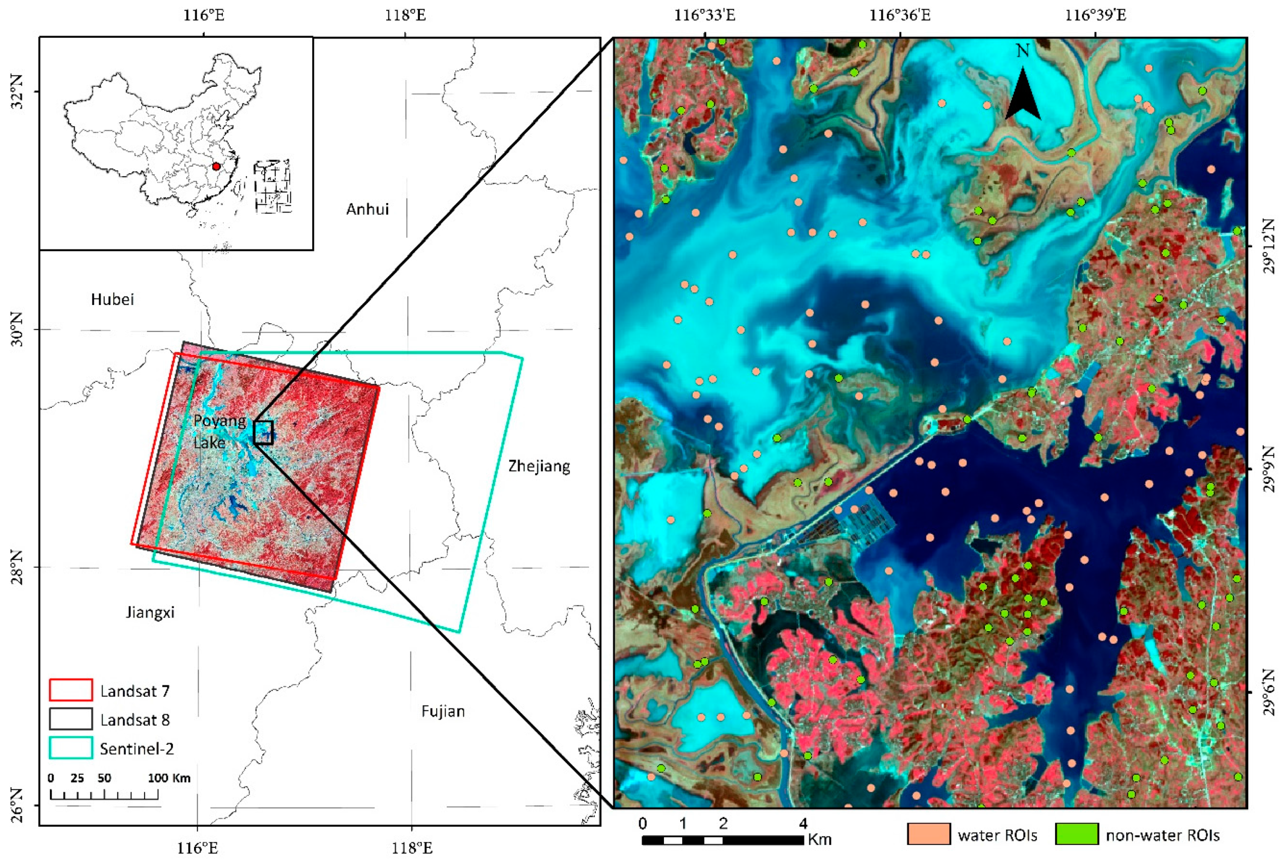
2.1. Study Area

We chose a case region in the Poyang Lake Basin as our study area. Poyang Lake is the largest freshwater lake in China, and is located in the north of the Jiangxi Province and the south-west border of the Anhui Province. The study area was selected deliberately to ensure that the water surface there remains submerged throughout the year. Relatively shallow and deep freshwater bodies both exist in the study area, and the water bodies in the northern half are shallower than those in the southern half. We also made sure that the case region had effective observations from Landsat 7 ETM+, Landsat 8 OLI, and Sentinel-2 MSI. The detailed location is shown in Figure 1.

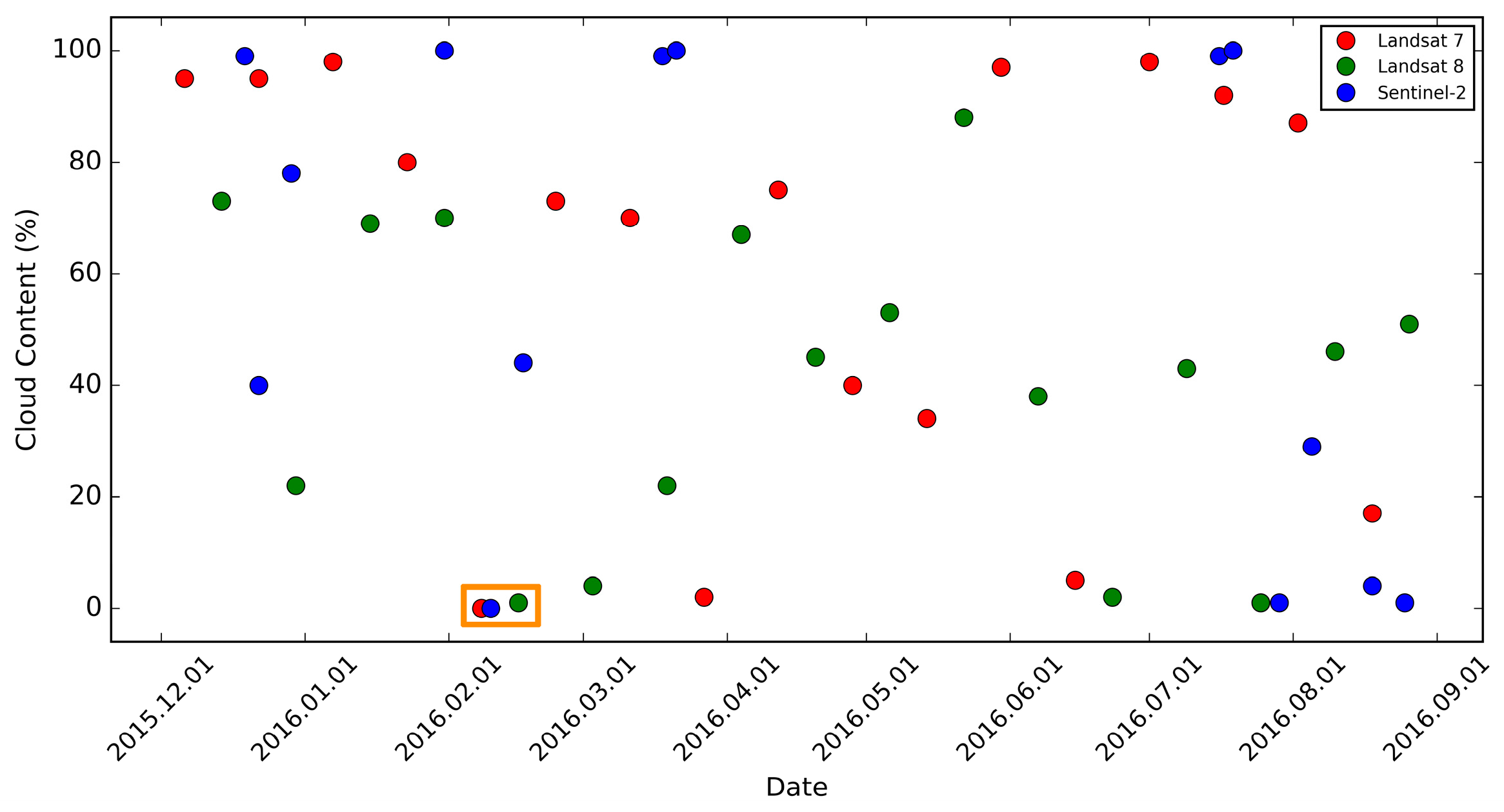
2.2. Data Acquisition and Processing

The Landsat 7 satellite is equipped with the Enhanced Thematic Mapper Plus (ETM+), including seven 30 m visible, near-infrared, and shortwave infrared bands, one 60 m thermal band, and one 15 m panchromatic band (Table 1). The Landsat 8 OLI satellite carries two Earth observing sensors of the Operational Land Imager (OLI) and the Thermal Infrared Sensor (TIRS), and the OLI collects image data for nine spectral bands with a spatial resolution of 30 m (15 m panchromatic band) and the TIRS collects image data for two thermal infrared spectral bands with a spatial resolution of 100 m. Both sensors provide a 15-degree field-of-view covering a 185 km across-track ground swath from an altitude of 705 km [46]. Sentinel-2 carries the Multi Spectral Instrument (MSI) with 13 bands covering the visible, NIR, and SWIR wavelength regions, including four 10 m visible and near-infrared bands, six 20 m vegetation red edge and short wave infrared bands, and three 60 m coastal aerosol, water vapor, and SWIR-Cirrus bands [47]. The band comparison of the three sensors (Landsat 7 ETM+, Landsat 8 OLI, and Sentinel-2 MSI) is shown in Table 1. The sun zenith angles of the selected Landsat 7 ETM+, Landsat 8 OLI, and Sentinel-2 MSI images were 50.46°, 48.41°, and 47.80°, respectively, while the sun azimuth angles were 147.50°, 145.23°, and 154.01°, respectively.
The water storage of lakes may be different over time, even in different days during a month. In order to make the water level consistent during the study period, the time selection requirement of images was strict in this study. Images of the three sensors (Landsat 7 ETM+, Landsat 8 OLI, and Sentinel-2 MSI) in the same or close period with less cloud coverage were chosen for this specific study. To achieve this aim, we checked all the availability and cloud percentages of the three datasets during their overlaid period (2015 December–present, Figure 2). As the surface water body extents may change quickly, we selected a period within which all the three kinds of quantified (low cloud coverage) images were available. Finally, we selected the images of Landsat 7 ETM+ (8 February 2016, Path/Row = 121/40), Landsat 8 OLI (16 February 2016, Path/Row = 121/40), and the Sentinel-2 MSI image (10 February 2016). The Level 1 Terrain Corrected (L1T) products of Landsat 7 and 8 surface reflectance data were derived from the U.S. Geological Survey (USGS) [48]. The Sentinel-2 MSI image was downloaded from the Sentinel Scientific Data Hub web site as a Level 1C (L1C) product. The Sentinel-2 L1C products were provided in Standard Archive Format for Europe (SAFE) file format [49], and the products were Top Of Atmosphere (TOA) reflectance data [50,51], with 12-bit dynamic range, and each image was in the Universal Transverse Mercator (UTM) map projection. We used the Sen2Cor algorithm on the SentiNel Application Platform (SNAP) developed by European Space Agency (ESA) to perform atmospheric correction to convert the images into product 2A which is the Bottom Of Atmosphere (BOA) reflectance data [48,52]. The Sentinel-2 MSI data has multiple bands, and the resolutions of the shortwave infrared bands (20 m) were different from that of the visible and near infrared bands (10 m) [53,54,55]. In order to make the Sentinel-2 data and Landsat data comparable, we resampled the visible and near infrared bands to 20 m to conduct further comparisons in this study. Before calculating the water indices, we used the nearest neighbor approach to resample the data of the visible and NIR bands to make the resolutions of the six bands used in this study consistent.

2.3. Methods

2.3.1. Water Index-Based Approaches

The index TCW developed by Crist [35,36] used all the six bands together with the coefficients empirically determined through analyzing both the simulated and actual data [36,56]. Due to the theory that water absorbs almost all incident radiant flux while the land surface reflects significant amounts of energy in near- and shortwave-infrared bands, and the reflectance in the green band is much higher for water compared to the land surface, McFeeters [37] put forward the NDWI using the value of the green band minus the near-infrared (NIR) band, divided by the sum of the two bands. As a result, water features have positive values and thus are enhanced, while the land surface has zero or negative values and is therefore suppressed or eliminated. However, water bodies are often mixed with built-up land noises in NDWI-images due to similar reflectance characteristics in the green and NIR bands between the water and built-up land. Xu [38] proposed the mNDWI by replacing the NIR band with SWIR-1 based on the above theory, achieving a satisfied result in suppressing built-up land noise. Due to water bodies having a relatively low reflectance, especially in the NIR to SWIR bands, Al-Khudhairy et al. [40] developed the Sum457 using the NIR, SWIR-1, and SWIR-2 bands of the Landsat Thematic Mapper (TM) data to delineate water bodies. Xiao et al. [57] developed the LSWI by considering the two bands of NIR and SWIR to estimate water content of the land surface. AWEI was developed by Feyisa et al. [41] to extract surface water with improved accuracy, and the coefficients that were used and the combinations of the chosen bands were determined based on critical examination of the reflectance properties of various land cover types.
In this study, we used nine water index-based algorithms, based on six water indices (TCW, NDWI, mNDWI, SNN, AWEI, and LSWI) or the combination of the water index and vegetation index, as well as three different sensors (Landsat 7 ETM+, Landsat 8 OLI, and Sentinel-2 MSI) of data to extract open surface water bodies. More detailed information about the open surface water body mapping algorithms in this study can be found in Table 2.

2.3.2. Validation and Method Comparison
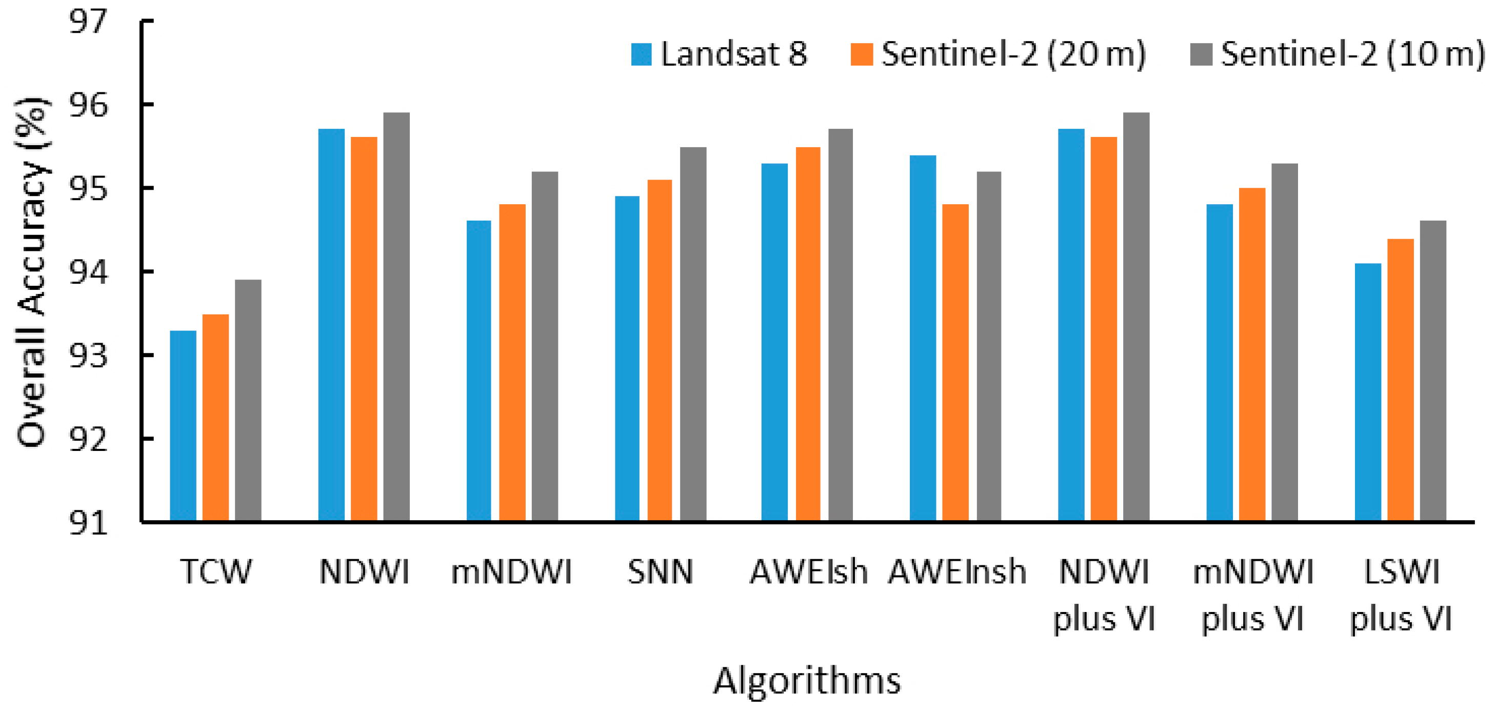
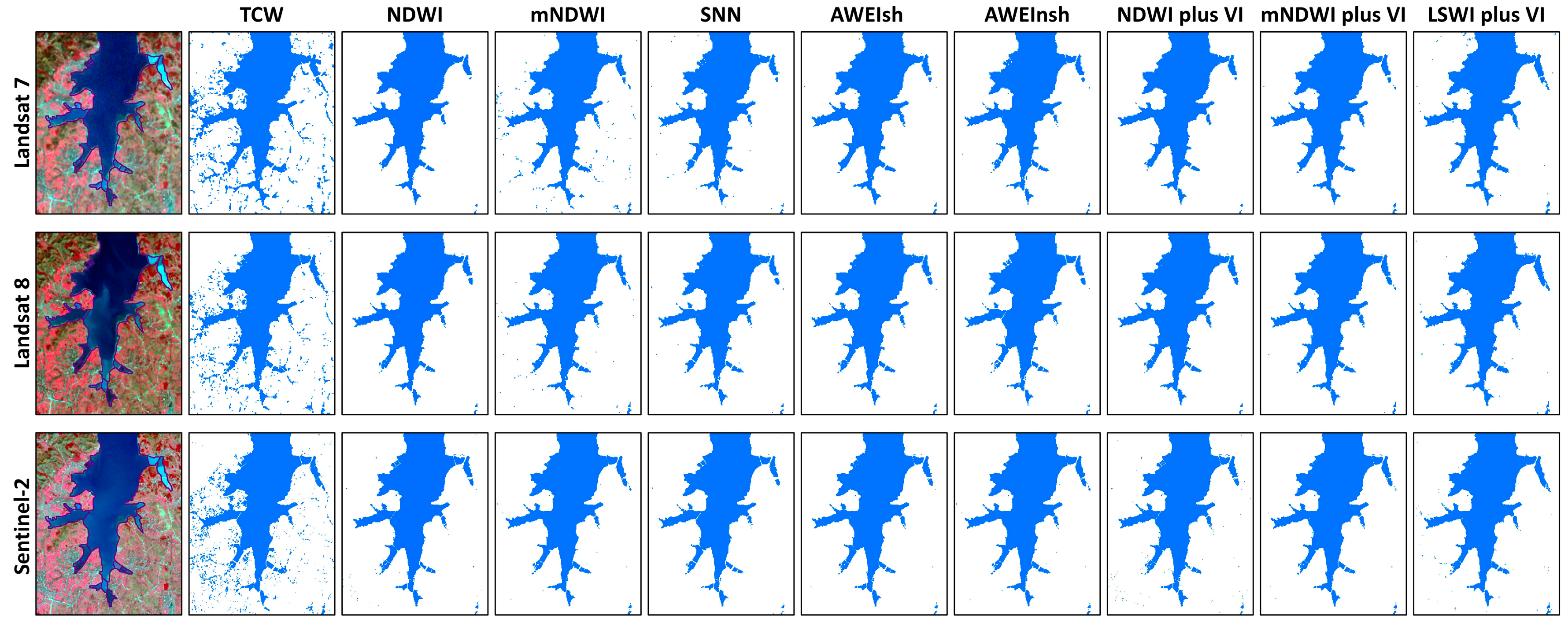
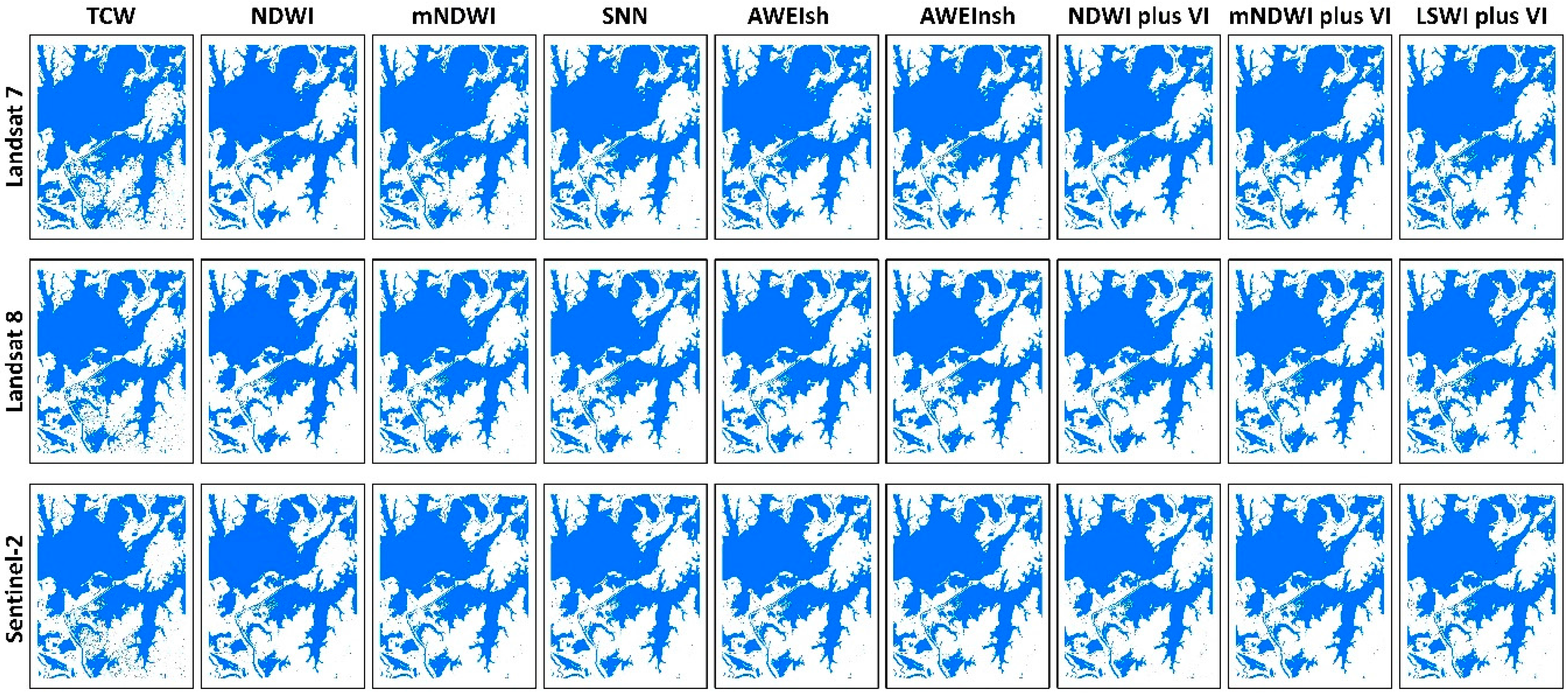
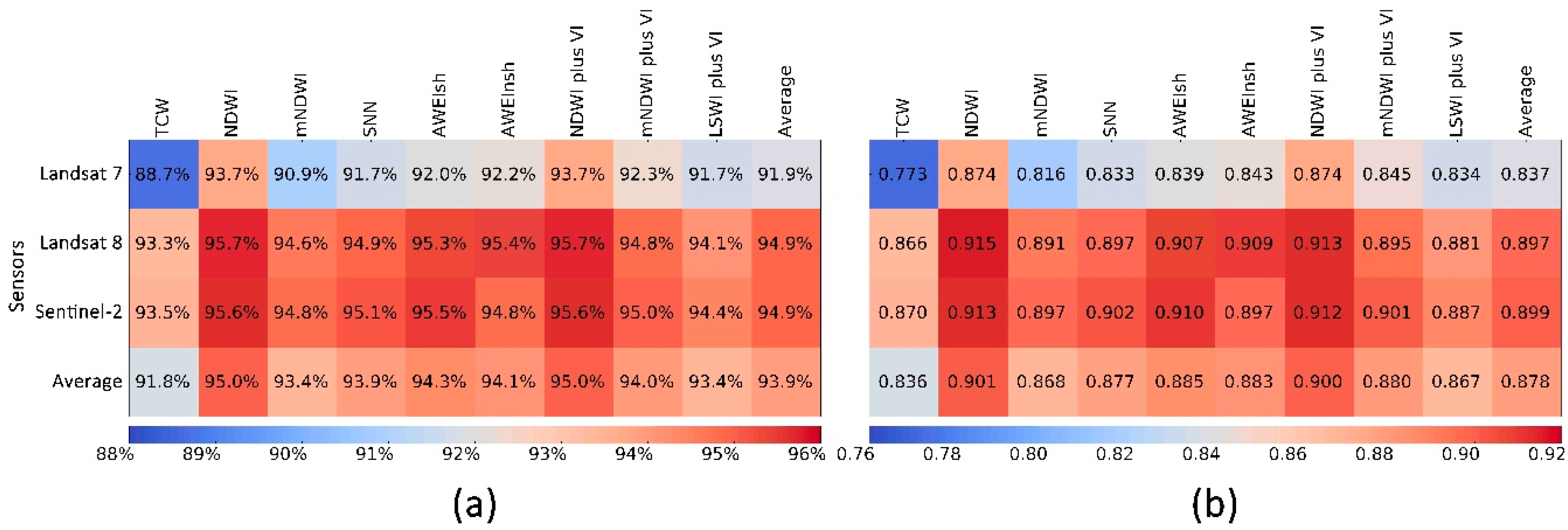
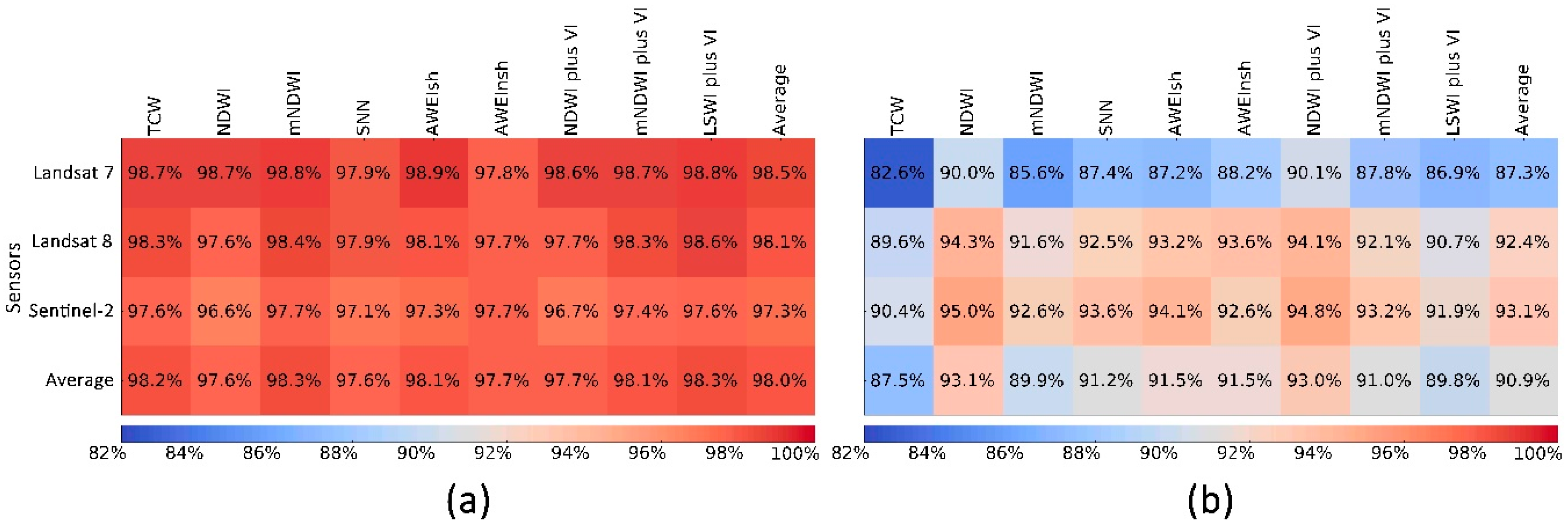
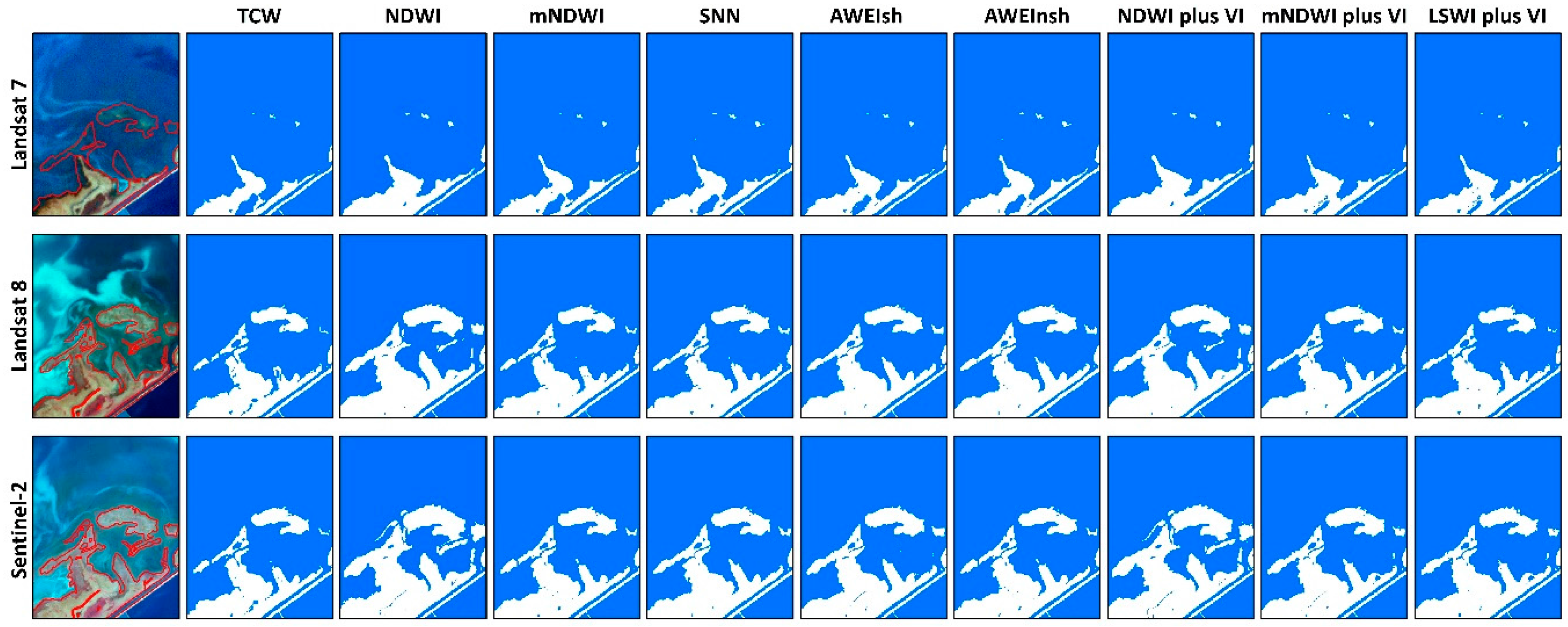
The open surface water body mapping results from the different approaches and sensors were evaluated by comparing against the very high resolution (VHR) imagery. In order to guarantee the temporal consistency of the results and ground truth data, we chose the reference VHR images obtained within ±8 days around the study period. A stratified random sampling method was used for the collection of the reference data. A primary water/non-water map was used to set up the strata, then 150 random points were generated in each stratum, and the sample numbers matched the proportions of the water and non-water areas. Then the buffers (circles of 100 m radius) of those points were generated as region of interests (ROIs) and used to be interpreted with the VHR images from the DigitalGlobe, Centre National d'Etudes Spatiales (CNES)/Astrium on the Google Earth platform, and Gaofen-3 (GF-3) for the recognition of land cover information. We deleted the ROIs with mixed pixels by visually checking the Google Earth platform. Finally, a total of 98 water and 93 non-water body ROIs were chosen (Figure 1). Confusion matrices for all the results from the combinations of the three sensors and nine algorithms were generated on the ENVI 5.3 software for accuracy assessment.

3. Results

The resultant open surface water body maps from the 27 combinations of the nine algorithms and three sensors are shown in Figure 3. Visually, all the results showed similar patterns of water bodies, while the Landsat-7 based results showed higher water areas than that from the other two sensors. Overall accuracies and Kappa coefficients are shown in Figure 4. All the results had an average overall accuracy of 93.9%, ranging from 88.7% to 95.7%. The two lowest accuracies were from the combinations of the TCW-based algorithm and Landsat 7 ETM+ data (TCW + Landsat 7 ETM+ for abbreviation) and the mNDWI + Landsat 7 ETM+; while the two highest accuracies were from the combinations of the NDWI + Landsat 8 OLI and the NDWI plus VI + Landsat 8 OLI. There was a small difference in the Kappa coefficients of the two methods with the highest overall accuracies (95.7%), the combination of the NDWI + Landsat 8 OLI had a Kappa coefficient of 0.915 while the combination of the NDWI plus VI + Landsat 8 OLI had a slightly lower Kappa coefficient of 0.913.
In terms of the performances of the nine algorithms, the NDWI-based algorithm and NDWI plus VI-based algorithm were stable and they shared the same highest overall accuracy for each sensor, while the TCW-based algorithm had the lowest accuracy for each sensor. Both the NDWI-based algorithm and NDWI plus VI-based algorithm had the same highest average overall accuracy of the three sensors (95.0%), followed by those algorithms based on AWEIsh (94.3%), AWEInsh (94.1%), mNDWI plus VI (94.0%), SNN (93.9%), mNDWI (93.4%), and LSWI plus VI (93.4%), while the TCW-based algorithm had the lowest average overall accuracy of 91.8%. The NDWI-based algorithm and the NDWI plus VI-based algorithm had high Kappa coefficients of ~0.90 for the three sensors. Specifically, the NDWI-based algorithm and NDWI plus VI-based algorithm had the same Kappa coefficients (0.874) when using Landsat 7 ETM+ data; while the Kappa coefficient was higher (~0.91) with a slight difference when using the Landsat 8 OLI and Sentinel-2 MSI data.
We also found different sensitivities of water body mapping for the three sensors. Landsat 8 OLI performed best with the highest overall accuracy (95.7%), followed by Sentinel-2 MSI (95.6%) and Landsat 7 ETM+ (93.7%). The average overall accuracies of the nine algorithms for Landsat 8 OLI was the same as that for Sentinel-2 MSI (94.9%), while the value for Landsat 7 ETM+ was the lowest (91.9%). The average Kappa coefficients of the nine algorithms for Sentinel-2 MSI was the highest (0.899), immediately followed by that for Landsat 8 OLI (0.897), and Landsat 7 ETM+ had a lower Kappa coefficient (0.837). Note that the Landsat 8 OLI based results always had higher overall accuracies than that of Landsat 7 ETM+ for all the algorithms, which implies the reliability of the improved design of the Landsat 8 OLI bandwidth.
For each algorithm, the omission error using the Landsat 7 ETM+ data was the lowest among the three kinds of data, and the producer accuracy using the Landsat 7 ETM+ data was slightly higher than those using the Landsat 8 OLI data and Sentinel-2 MSI data (Figure 5a). As the commission error of each algorithm using Landsat 7 ETM+ data was much higher than that using the other two kinds of data, the user accuracy of each algorithm using the Landsat 8 OLI data and Sentinel-2 MSI data was higher than that using the Landsat 7 ETM+ data to a large extent (Figure 5b). It can be seen that the user accuracy difference among the three sensors for each algorithm was the main factor that caused the lowest accuracy of each algorithm using the Landsat 7 ETM+ data. From the perspective of algorithm performance, the producer accuracies of the NDWI-based algorithm and the NDWI plus VI-based algorithm were not the highest for each sensor, and the producer accuracy difference of the nine algorithms was subtle; however, the user accuracy of the NDWI-based and NDWI plus VI-based algorithms was much higher than that of the other algorithms, and the user accuracy differences of all of the nine algorithms were larger than those of the producer accuracies of all the algorithms. That was the main reason for why the NDWI-based and NDWI plus VI-based algorithms performed best with the same highest overall accuracy among the nine algorithms, while the TCW-based algorithm performed the worst with the lowest accuracy due to the largest commission error in the study area.

4. Discussion

4.1. Comparison of Different Water Indices in Water Body Extraction

Among the various water indices, we found that the NDWI-based and NDWI plus VI-based algorithms had slightly higher accuracies in our study area, no matter which sensor was used. Xu [38] proposed the mNDWI by replacing the NIR band with SWIR at the base of NDWI, and demonstrated that mNDWI can largely suppress the noise of built-up lands better than NDWI, especially in the areas where buildings dominate. In this specific study, we did not find a higher accuracy of the mNDWI-based algorithm compared to the NDWI-based algorithm for each sensor, probably because there were limited mixed water and built-up land pixels in the study area (Figure 1). The user accuracy of the NDWI-based algorithm was larger than that of the mNDWI-based algorithm, so the commission error of NDWI was lower than that of mNDWI; which implied that the mNDWI-based algorithm could have better performance of water body mapping in complex landscapes, while the NDWI had higher sensitivity for water body extraction in pure open surface water body regions. Menarguez [43] tried to improve the performances of the NDWI- or mNDWI-based algorithms by involving vegetation indices (EVI and NDVI), that could help take care of the mixed pixels of water and vegetation. That could be particularly meaningful when used in flood monitoring, e.g., paddy rice transplant monitoring [42,58,59].
TCW achieved the lowest accuracy among the nine algorithms no matter which data source was used. Due to the many non-water pixels that were mistakenly classified into water pixels, the commission error of TCW was larger than that of the other eight algorithms, so the user accuracy was the lowest among the nine algorithms (Figure 5b).
In order to minimize the errors of atmospheric correction, Beeri et al. [39] proposed an integrated indicator by considering Sum457, ND5723, and ND571. We found this integrated indicator performed well for Landsat 8 OLI (OA = 95.7%); however, it showed a lower accuracy compared to the NDWI-based algorithms when using the Landsat 7 ETM+ and Sentinel-2 MSI data. This study implied that the integrated approach by considering more indices could not necessarily be more robust than a simple combination of NIR and green bands in the identification of open surface water bodies.
As an initial effort, we selected a simple and ideal case region, generally covered by pure open surface water bodies. There was no shadow area due to the flat terrain, and no high-albedo surfaces such as snow and ice because of the warm weather in the Poyang Lake Basin. Also, very limited urban areas existed in the area. Therefore, we found both AWEInsh- and AWEIsh-based algorithms achieved reasonably high accuracies.

4.2. Comparison of Different Sensors in Water Body Extraction

As for the performance comparison among the three sensors, the Landsat 8 OLI and Sentinel-2 MSI performed better than the Landsat 7 ETM+, and the average overall accuracy of all of the nine algorithms using the Landsat 8 OLI data was almost the same as that using the Sentinel-2 MSI data (Average OA = 94.9%), while the value of Landsat 7 ETM+ was lower (91.9%). The overall accuracies of all of the nine algorithms using the Landsat 8 OLI data were higher than that using the Landsat 7 ETM+ data, and was due to the significant improvements of several aspects made in Landsat 8 OLI compared to Landsat 7 ETM+. Landsat 8 OLI improved the signal-to-noise ratio (SNR) [60] and the measurement of subtle variability in the ground by quantizing data to twelve bits as compared to the eight-bit data produced by Landsat 7 ETM+ [23,61].
The highly reflective surfaces such as snow, clouds, and sun-glint over water bodies may saturate, and especially the sun-glint over water bodies is an important factor that could cause the saturation of the reflective wavebands due to the flat terrain in the Poyang Lake Basin. The visible bands in Landsat 7 ETM+ tend to saturate more frequently compared to the bands in Landsat 8 OLI, which improved the dynamic range to reduce band saturation over highly reflective objects [62]. Regarding the improvements of the waveband design in Landsat 8 OLI, the OLI bands are spectrally narrower and cover different spectral ranges compared to Landsat 7 ETM due to the band edges that have been modified to avoid atmospheric absorption features, which can add additional uncertainties to the reflected wave from water bodies. The most significant change is that the NIR and SWIR-1 bands of Landsat 8 OLI are substantially narrower than those of Landsat 7 ETM+, which obviously avoids a water absorption feature that occurs in the NIR band and SWIR-1 band of Landsat 7 ETM+. Generally, the SNR is smaller in the narrower band, but Landsat 8 OLI overcome this limitation by implementing a pushbroom imager, allowing for longer dwell times and a greater range of the sensed signal. So, the SNR of Landsat 8 OLI is 6 to 10 times better than that of Landsat 7 ETM+ for the different spectral bands, which has allowed narrowing down of its spectral bandwidths to avoid atmospheric absorption to the reflected wave from water bodies [61,62]. An additional cirrus band of Landsat 8 (1.36–1.38 μm) and Sentinel-2 (1.365–1.385 μm) can be used to detect clouds, which is especially helpful for detecting high altitude clouds [62,63,64,65]. Some water indices were defined to be calculated by the surface reflectance data of each band, so the original TOA reflectance data needs to conduct atmospheric corrections to be converted into surface reflectance data, to remove the impacts of several factors such as atmospheric gases and aerosols in space. As the band designs of Landsat 8 OLI were more focused on minimizing atmospheric impacts, and the atmospheric correction models of Landsat 8 OLI have been improved compared to Landsat 7 ETM+ [61,66], the surface reflectance data of Landsat 8 OLI is closer to the true values of the surface reflectance compared to Landsat 7 ETM+. Based on the above points, we concluded that Landsat 8 OLI is more applicable to extract water bodies than Landsat 7 ETM+ [67].
In terms of the performance difference between Landsat 8 OLI and Sentinel-2 MSI, the overall performance was almost the same. The average of the overall accuracy of all of the nine algorithms using the Landsat 8 OLI data was the same as that using the Sentinel-2 MSI data (Average OA = 94.9%). This could be attributed to the similar band wavelength of the two sensors, specifically, the central wavelength of band SWIR-1 in both sensors is 1.61 µm. The radiometric resolution of Sentinel-2 MSI is as same as Landsat 8 OLI (12-bit) [68] despite the higher spatial resolution of Sentinel-2 MSI.
This study showed a similar performance between the 20 m Sentinel-2 data and the 30 m Landsat 8 data. Note that we compared Sentinel-2 and Landsat 8 using different resolutions of data. That is, the capability of the Sentinel-2 data could be partly attributed to the higher spatial resolution. Moreover, we added more analyses based on the 10 m Sentinel-2 data (resampling 20 m SWIR Bands into 10 m resolution) and found that the 10 m Sentinel-2 results had an improved accuracy compared to those based on the 20 m Sentinel-2 data and the 30 m Landsat 8 data (Figure 6).
More variables such as the seasonal and daily difference of the sun angle, atmospheric composition, changes in water body properties, and even the choice of atmospheric correction methods may also affect the accuracy of water body extraction. Those are beyond the scope of this specific study and need to be explored in a future study.

4.3. Sensitivities of Sensors and Water Body Mapping Algorithms in Different Water Conditions

As for various water conditions, different sensors and water mapping algorithms could have different performances. We compared the results in a shallow water body area (Figure 7) where the bottom albedo could contribute to observed radiance and affect the accuracies of algorithms. As can be seen in Figure 7, Landsat 7 ETM+ performed the worst and a lot of non-water pixels were classified into water pixels in the shallow water body area where a large amount of silt sediments exist, which caused a high commission error. In the border region of water and land, Landsat 7 ETM+ also had higher commission errors (Figure 8).
Among the nine algorithms, the NDWI-based and NDWI plus VI-based algorithms performed better than the others in either shallow water conditions (Figure 7) or mixed water and land conditions (Figure 8), no matter which sensor was used. TCW performed worst with the lowest overall accuracy and user accuracy, as many built-up lands were identified as water bodies (Figure 8) and caused a high commission error. The mNDWI-based algorithm also had higher commission errors than that of the NDWI-based algorithm (Figure 8).
Different types of water bodies have different reflectance patterns [56]; for example, reflectance peaks occur in the green band for the water bodies with high concentrations of phytoplankton, while the water bodies with a high concentration of sediments such as silt have reflectance peaks in the red band. Given that each water index has its own specific combination of spectral bands, it would have a better performance in extracting a certain kind of water body. Thus it would not be effective to just use only one water index to extract the water bodies in a large scale region where various types of water bodies are mixed. It could achieve a higher accuracy in large scale water body mapping using a combination of different water indices. More characteristics of those water indices and their sensitivities to different water cover types should be further explored and compared in the future.

5. Conclusions

In this study, we evaluated the performances of 27 water body extraction strategies by combining nine water index-based algorithms and three sensors in an open surface water body region inside the Poyang Lake Basin. The overall accuracy, Kappa coefficient, producer accuracy, and user accuracy for each result were calculated to evaluate the performance of each method. We found that all the methods generally had reasonable overall accuracies ranging from 88.7% to 95.7% and Kappa Coefficients ranging from 0.77 to 0.92. The two lowest accuracies were from the combinations of TCW + Landsat 7 ETM+ and mNDWI + Landsat 7 ETM+; while the two highest accuracies were from the combinations of NDWI + Landsat 8 OLI and NDWIplusVI + Landsat 8 OLI. The combinations of NDWI + Landsat 8 OLI as well as NDWIplusVI + Landsat 8 OLI had the highest accuracies.
Among the three sensors, Landsat 8 OLI and Sentinel-2 MSI performed better with higher accuracies than Landsat 7 ETM+ in the extraction of water bodies for almost all of the algorithms. Regarding the performance difference between Landsat 8 OLI and Sentinel-2 MSI, their accuracies were almost the same. As for the performances of the nine algorithms, the NDWI- and NDWI plus VI-based algorithms performed best with the highest average overall accuracy (95.0%) and Kappa coefficient (0.913–0.915), followed by the algorithms based on AWEIsh, AWEInsh, mNDWI plus VI, SNN, mNDWI, LSWI plus VI, and TCW. However, these findings may not able to be simply applied to other regions, as they were based on the limited study area dominated by the pure open surface water body. The performances of those water index based algorithms in more complex situations, e.g., the mixed water + soil, or mixed water + vegetation conditions, could be different and should be explored in future studies.
Above all, all the three sensors and nine algorithms based on different water indices had reasonable good performances in open surface water body mapping, while Landsat 8 and Sentinel-2 as well as NDWI had extraordinary advantages for accurate water body mapping in the study area. This study provided valuable implications for the selection of water indices and sensors for large scale open surface water body mapping efforts.

Acknowledgments

This study is funded by the Key Research Program of Frontier Sciences, the Chinese Academy of Sciences (QYZDB-SSW-DQC005), the “Thousand Youth Talents Plan”, the National Natural Science Foundation of China (41501117), the National Science Foundation EPSCoR program (OIA-1301789), and the National Institutes of Health NIAID (1R01AI101028-01A2).

Author Contributions

Jinwei Dong, Xiangming Xiao, and Yan Zhou conceived and designed the experiments; Yan Zhou performed the experiments; Jinwei Dong, Xiangming Xiao, Yan Zhou, Tong Xiao, Zhiqi Yang, Guosong Zhao, Zhenhua Zou, and Yuanwei Qin analyzed the data and wrote the paper.

Conflicts of Interest

The authors declare no conflict of interest. The founding sponsors had no role in the design of the study; in the collection, analyses, or interpretation of data; in the writing of the manuscript, and in the decision to publish the results.

References

  1. Tao, S.; Fang, J.; Zhao, X.; Zhao, S.; Shen, H.; Hu, H.; Tang, Z.; Wang, Z.; Guo, Q. Rapid loss of lakes on the Mongolian Plateau. PNAS 2015, 112, 2281–2286. [Google Scholar] [CrossRef] [PubMed]
  2. Yang, Y.; Liu, Y.; Zhou, M.; Zhang, S.; Zhan, W.; Sun, C.; Duan, Y. Landsat 8 OLI image based terrestrial water extraction from heterogeneous backgrounds using a reflectance homogenization approach. Remote Sens. Environ. 2015, 171, 14–32. [Google Scholar] [CrossRef]
  3. Sharma, R.; Tateishi, R.; Hara, K.; Nguyen, L. Developing Superfine Water Index (SWI) for Global Water Cover Mapping Using MODIS Data. Remote Sens. 2015, 7, 13807–13841. [Google Scholar] [CrossRef]
  4. Anderson, M.C.; Allen, R.G.; Morse, A.; Kustas, W.P. Use of Landsat thermal imagery in monitoring evapotranspiration and managing water resources. Remote Sens. Environ. 2012, 122, 50–65. [Google Scholar] [CrossRef]
  5. Palmer, S.C.J.; Kutser, T.; Hunter, P.D. Remote sensing of inland waters: Challenges, progress and future directions. Remote Sens. Environ. 2015, 157, 1–8. [Google Scholar] [CrossRef]
  6. Stokstad, E. High Court Asks Army Corps To Measure Value of Wetlands. Science 2006, 312, 1870. [Google Scholar] [CrossRef] [PubMed]
  7. Yamazaki, D.; Trigg, M.A.; Ikeshima, D. Development of a global ~90m water body map using multi-temporal Landsat images. Remote Sens. Environ. 2015, 171, 337–351. [Google Scholar] [CrossRef]
  8. Du, Y.; Zhang, Y.; Ling, F.; Wang, Q.; Li, W.; Li, X. Water Bodies’ Mapping from Sentinel-2 Imagery with Modified Normalized Difference Water Index at 10-m Spatial Resolution Produced by Sharpening the SWIR Band. Remote Sens. 2016, 8, 354. [Google Scholar] [CrossRef]
  9. Du, J.; Kimball, J.S.; Jones, L.A.; Watts, J.D. Implementation of satellite based fractional water cover indices in the pan-Arctic region using AMSR-E and MODIS. Remote Sens. Environ. 2016, 184, 469–481. [Google Scholar] [CrossRef]
  10. Liu, J.; Zhang, Y.; Yuan, D.; Song, X. Empirical Estimation of Total Nitrogen and Total Phosphorus Concentration of Urban Water Bodies in China Using High Resolution IKONOS Multispectral Imagery. Water 2015, 7, 6551–6573. [Google Scholar] [CrossRef]
  11. Donchyts, G.; Schellekens, J.; Winsemius, H.; Eisemann, E.; van de Giesen, N. A 30 m Resolution Surface Water Mask Including Estimation of Positional and Thematic Differences Using Landsat 8, SRTM and OpenStreetMap: A Case Study in the Murray-Darling Basin, Australia. Remote Sens. 2016, 8, 386. [Google Scholar] [CrossRef]
  12. Santoro, M.; Wegmüller, U.; Lamarche, C.; Bontemps, S.; Defourny, P.; Arino, O. Strengths and weaknesses of multi-year Envisat ASAR backscatter measurements to map permanent open water bodies at global scale. Remote Sens. Environ. 2015, 171, 185–201. [Google Scholar] [CrossRef]
  13. Polizzotto, M.L.; Kocar, B.D.; Benner, S.G.; Sampson, M.; Fendorf, S. Near-surface wetland sediments as a source of arsenic release to ground water in Asia. Nature 2008, 454, 505–508. [Google Scholar] [CrossRef] [PubMed]
  14. Ji, L.; Zhang, L.; Wylie, B. Analysis of Dynamic Thresholds for the Normalized Difference Water Index. Photogramm. Eng. Remote Sens. 2009, 75, 1307–1317. [Google Scholar] [CrossRef]
  15. Chandrasekar, K.; Sesha Sai, M.V.R.; Roy, P.S.; Dwevedi, R.S. Land Surface Water Index (LSWI) response to rainfall and NDVI using the MODIS Vegetation Index product. Int. J. Remote Sens. 2010, 31, 3987–4005. [Google Scholar] [CrossRef]
  16. Crasto, N.; Hopkinson, C.; Forbes, D.L.; Lesack, L.; Marsh, P.; Spooner, I.; van der Sanden, J.J. A LiDAR-based decision-tree classification of open water surfaces in an Arctic delta. Remote Sens. Environ. 2015, 164, 90–102. [Google Scholar] [CrossRef]
  17. Barrett, D.; Frazier, A. Automated Method for Monitoring Water Quality Using Landsat Imagery. Water 2016, 8, 257. [Google Scholar] [CrossRef]
  18. Torres-Rua, A.; Ticlavilca, A.; Bachour, R.; McKee, M. Estimation of Surface Soil Moisture in Irrigated Lands by Assimilation of Landsat Vegetation Indices, Surface Energy Balance Products, and Relevance Vector Machines. Water 2016, 8, 167. [Google Scholar] [CrossRef]
  19. Giustarini, L.; Hostache, R.; Kavetski, D.; Chini, M.; Corato, G.; Schlaffer, S.; Matgen, P. Probabilistic Flood Mapping Using Synthetic Aperture Radar Data. IEEE Trans. Geosci. Remote Sens. 2016, 54, 1–12. [Google Scholar] [CrossRef]
  20. Tulbure, M.G.; Broich, M.; Stehman, S.V.; Kommareddy, A. Surface water extent dynamics from three decades of seasonally continuous Landsat time series at subcontinental scale in a semi-arid region. Remote Sens. Environ. 2016, 178, 142–157. [Google Scholar] [CrossRef]
  21. Pahlevan, N.; Schott, J.R. Characterizing the relative calibration of Landsat-7 (ETM+) visible bands with Terra (MODIS) over clear waters: The implications for monitoring water resources. Remote Sens. Environ. 2012, 125, 167–180. [Google Scholar] [CrossRef]
  22. Vogelmann, J.E.; Gallant, A.L.; Shi, H.; Zhu, Z. Perspectives on monitoring gradual change across the continuity of Landsat sensors using time-series data. Remote Sens. Environ. 2016, 185, 258–270. [Google Scholar] [CrossRef]
  23. Wulder, M.A.; White, J.C.; Loveland, T.R.; Woodcock, C.E.; Belward, A.S.; Cohen, W.B.; Fosnight, E.A.; Shaw, J.; Masek, J.G.; Roy, D.P. The global Landsat archive: Status, consolidation, and direction. Remote Sens. Environ. 2016, 185, 271–283. [Google Scholar] [CrossRef]
  24. Pekel, J.F.; Cottam, A.; Gorelick, N.; Belward, A.S. High-resolution mapping of global surface water and its long-term changes. Nature 2016, 540, 418–422. [Google Scholar] [CrossRef] [PubMed]
  25. Sheng, Y.; Shah, C.A.; Smith, L.C. Automated Image Registration for Hydrologic Change Detection in the Lake-Rich Arctic. IEEE Geosci. Remote Sens. Lett. 2008, 5, 414–418. [Google Scholar] [CrossRef]
  26. Sivanpillai, R.; Miller, S.N. Improvements in mapping water bodies using ASTER data. Ecol. Inf. 2010, 5, 73–78. [Google Scholar] [CrossRef]
  27. Huang, C.; Chen, Y.; Wu, J. Mapping spatio-temporal flood inundation dynamics at large river basin scale using time-series flow data and MODIS imagery. Int. J. Appl. Earth Obs. Geoinf. 2014, 26, 350–362. [Google Scholar] [CrossRef]
  28. Li, W.; Du, Z.; Ling, F.; Zhou, D.; Wang, H.; Gui, Y.; Sun, B.; Zhang, X. A Comparison of Land Surface Water Mapping Using the Normalized Difference Water Index from TM, ETM+ and ALI. Remote Sens. 2013, 5, 5530–5549. [Google Scholar] [CrossRef]
  29. Li, W.; Qin, Y.; Sun, Y.; Huang, H.; Ling, F.; Tian, L.; Ding, Y. Estimating the relationship between dam water level and surface water area for the Danjiangkou Reservoir using Landsat remote sensing images. Remote Sens. Lett. 2015, 7, 121–130. [Google Scholar] [CrossRef]
  30. Xie, H.; Luo, X.; Xu, X.; Tong, X.; Jin, Y.; Pan, H.; Zhou, B. New hyperspectral difference water index for the extraction of urban water bodies by the use of airborne hyperspectral images. J. Appl. Remote Sens. 2014, 8, 085098. [Google Scholar] [CrossRef]
  31. Hui, F.; Xu, B.; Huang, H.; Yu, Q.; Gong, P. Modelling spatial-temporal change of Poyang Lake using multitemporal Landsat imagery. Int. J. Remote Sens. 2008, 29, 5767–5784. [Google Scholar] [CrossRef]
  32. Ji, L.; Geng, X.; Sun, K.; Zhao, Y.; Gong, P. Target Detection Method for Water Mapping Using Landsat 8 OLI/TIRS Imagery. Water 2015, 7, 794–817. [Google Scholar] [CrossRef]
  33. Ouma, Y.O.; Tateishi, R. A water index for rapid mapping of shoreline changes of five East African Rift Valley lakes: An empirical analysis using Landsat TM and ETM+ data. Int. J. Remote Sens. 2006, 27, 3153–3181. [Google Scholar] [CrossRef]
  34. Du, Z.; Li, W.; Zhou, D.; Tian, L.; Ling, F.; Wang, H.; Gui, Y.; Sun, B. Analysis of Landsat-8 OLI imagery for land surface water mapping. Remote Sens. Lett. 2014, 5, 672–681. [Google Scholar] [CrossRef]
  35. Crist, E.P. A TM Tasseled Cap Equivalent Transformation for Reflectance Factor Data. Remote Sens. Environ. 1985, 17, 301–306. [Google Scholar] [CrossRef]
  36. Crist, E.P.; Cicone, R.C. A Physically-Based Transformation of Thematic Mapper Data-The TM Tasseled Cap. IEEE Trans. Geosci. Remote Sens. 1984, 22, 256–263. [Google Scholar] [CrossRef]
  37. McFeeters, S.K. The use of the Normalized Difference Water Index (NDWI) in the delineation of open water features. Int. J. Remote Sens. 1996, 17, 1425–1432. [Google Scholar] [CrossRef]
  38. Xu, H. Modification of normalised difference water index (NDWI) to enhance open water features in remotely sensed imagery. Int. J. Remote Sens. 2006, 27, 3025–3033. [Google Scholar] [CrossRef]
  39. Beeri, O.; Phillips, R.L. Tracking palustrine water seasonal and annual variability in agricultural wetland landscapes using Landsat from 1997 to 2005. Glob. Chang. Biol. 2007, 13, 897–912. [Google Scholar] [CrossRef]
  40. Al-Khudhairy, D.; Leemhuis, C.; Hofhnann, V.; Shepherd, I.; Calaon, R.; Thompson, J.; Gavin, H.; Gasca-Tucker, D.; Zalldls, Q.; Bilas, G.; et al. Monitoring Wetland Ditch Water Levels Using Landsat TM and Ground-Based Measurements. Photogramm. Eng. Remote Sens. 2002, 608, 809–818. [Google Scholar]
  41. Feyisa, G.L.; Meilby, H.; Fensholt, R.; Proud, S.R. Automated Water Extraction Index: A new technique for surface water mapping using Landsat imagery. Remote Sens. Environ. 2014, 140, 23–35. [Google Scholar] [CrossRef]
  42. Dong, J.; Xiao, X.; Menarguez, M.A.; Zhang, G.; Qin, Y.; Thau, D.; Biradar, C.; Moore, B. Mapping paddy rice planting area in Northeastern Asia with Landsat 8 images, phenology-based algorithm and Google Earth Engine. Remote Sens. Environ. 2016, 185, 142–154. [Google Scholar] [CrossRef] [PubMed]
  43. Menarguez, M.A. Global Water Body Mapping from 1984 to 2015 Using Global High Resolution Multispectral Satellite Imagery; University of Oklahoma: Norman, OK, USA, 2015. [Google Scholar]
  44. Halabisky, M.; Moskal, L.M.; Gillespie, A.; Hannam, M. Reconstructing semi-arid wetland surface water dynamics through spectral mixture analysis of a time series of Landsat satellite images (1984–2011). Remote Sens. Environ. 2016, 177, 171–183. [Google Scholar] [CrossRef]
  45. Loveland, T.R.; Irons, J.R. Landsat 8: The plans, the reality, and the legacy. Remote Sens. Environ. 2016, 185, 1–6. [Google Scholar] [CrossRef]
  46. Irons, J.R.; Dwyer, J.L.; Barsi, J.A. The next Landsat satellite: The Landsat Data Continuity Mission. Remote Sens. Environ. 2012, 122, 11–21. [Google Scholar] [CrossRef]
  47. Yan, L.; Roy, D.; Zhang, H.; Li, J.; Huang, H. An Automated Approach for Sub-Pixel Registration of Landsat-8 Operational Land Imager (OLI) and Sentinel-2 Multi Spectral Instrument (MSI) Imagery. Remote Sens. 2016, 8, 520. [Google Scholar] [CrossRef]
  48. Novelli, A.; Aguilar, M.A.; Nemmaoui, A.; Aguilar, F.J.; Tarantino, E. Performance evaluation of object based greenhouse detection from Sentinel-2 MSI and Landsat 8 OLI data: A case study from Almería (Spain). Int. J. Appl. Earth Obs. Geoinf. 2016, 52, 403–411. [Google Scholar] [CrossRef]
  49. Roy, D.P.; Li, J.; Zhang, H.K.; Yan, L. Best practices for the reprojection and resampling of Sentinel-2 Multi Spectral Instrument Level 1C data. Remote Sens. Lett. 2016, 7, 1023–1032. [Google Scholar] [CrossRef]
  50. Storey, J.; Roy, D.P.; Masek, J.; Gascon, F.; Dwyer, J.; Choate, M. A note on the temporary misregistration of Landsat-8 Operational Land Imager (OLI) and Sentinel-2 Multi Spectral Instrument (MSI) imagery. Remote Sens. Environ. 2016, 186, 121–122. [Google Scholar] [CrossRef]
  51. Malenovský, Z.; Rott, H.; Cihlar, J.; Schaepman, M.E.; García-Santos, G.; Fernandes, R.; Berger, M. Sentinels for science: Potential of Sentinel-1, -2 and -3 missions for scientific observations of ocean, cryosphere, and land. Remote Sens. Environ. 2012, 120, 91–101. [Google Scholar] [CrossRef]
  52. Toming, K.; Kutser, T.; Laas, A.; Sepp, M.; Paavel, B.; Nõges, T. First Experiences in Mapping Lake Water Quality Parameters with Sentinel-2 MSI Imagery. Remote Sens. 2016, 8, 640. [Google Scholar] [CrossRef]
  53. Wang, Q.; Shi, W.; Li, Z.; Atkinson, P.M. Fusion of Sentinel-2 images. Remote Sens. Environ. 2016, 187, 241–252. [Google Scholar] [CrossRef]
  54. Herrmann, I.; Pimstein, A.; Karnieli, A.; Cohen, Y.; Alchanatis, V.; Bonfil, D.J. LAI assessment of wheat and potato crops by VENμS and Sentinel-2 bands. Remote Sens. Environ. 2011, 115, 2141–2151. [Google Scholar] [CrossRef]
  55. Van der Meer, F.D.; van der Werff, H.M.A.; van Ruitenbeek, F.J.A. Potential of ESA’s Sentinel-2 for geological applications. Remote Sens. Environ. 2014, 148, 124–133. [Google Scholar] [CrossRef]
  56. Fisher, A.; Flood, N.; Danaher, T. Comparing Landsat water index methods for automated water classification in eastern Australia. Remote Sens. Environ. 2016, 175, 167–182. [Google Scholar] [CrossRef]
  57. Xiao, X.; Boles, S.; Frolking, S.; Salas, W.; Moore, B., III; Li, C.; He, L.; Zhao, R. Observation of flooding and rice transplanting of paddy rice fields at the site to landscape scales in China using VEGETATION sensor data. Int. J. Remote Sens. 2002, 23, 3009–3022. [Google Scholar] [CrossRef]
  58. Dong, J.; Xiao, X.; Kou, W.; Qin, Y.; Zhang, G.; Li, L.; Jin, C.; Zhou, Y.; Wang, J.; Biradar, C.; et al. Tracking the dynamics of paddy rice planting area in 1986–2010 through time series Landsat images and phenology-based algorithms. Remote Sens. Environ. 2015, 160, 99–113. [Google Scholar] [CrossRef]
  59. Xiao, X.; Boles, S.; Liu, J.; Zhuang, D.; Frolking, S.; Li, C.; Salas, W.; Moore, B. Mapping paddy rice agriculture in southern China using multi-temporal MODIS images. Remote Sens. Environ. 2005, 95, 480–492. [Google Scholar] [CrossRef]
  60. Sheng, Y.; Song, C.; Wang, J.; Lyons, E.A.; Knox, B.R.; Cox, J.S.; Gao, F. Representative lake water extent mapping at continental scales using multi-temporal Landsat-8 imagery. Remote Sens. Environ. 2016, 185, 129–141. [Google Scholar] [CrossRef]
  61. Roy, D.P.; Kovalskyy, V.; Zhang, H.K.; Vermote, E.F.; Yan, L.; Kumar, S.S.; Egorov, A. Characterization of Landsat-7 to Landsat-8 reflective wavelength and normalized difference vegetation index continuity. Remote Sens. Environ. 2016, 185, 57–70. [Google Scholar] [CrossRef]
  62. Mishra, N.; Helder, D.; Barsi, J.; Markham, B. Continuous calibration improvement in solar reflective bands: Landsat 5 through Landsat 8. Remote Sens. Environ. 2016, 185, 7–15. [Google Scholar] [CrossRef]
  63. Senay, G.B.; Friedrichs, M.; Singh, R.K.; Velpuri, N.M. Evaluating Landsat 8 evapotranspiration for water use mapping in the Colorado River Basin. Remote Sens. Environ. 2016, 185, 171–185. [Google Scholar] [CrossRef]
  64. Zhu, Z.; Wang, S.; Woodcock, C.E. Improvement and expansion of the Fmask algorithm: Cloud, cloud shadow, and snow detection for Landsats 4–7, 8, and Sentinel 2 images. Remote Sens. Environ. 2015, 159, 269–277. [Google Scholar] [CrossRef]
  65. Hollstein, A.; Segl, K.; Guanter, L.; Brell, M.; Enesco, M. Ready-to-Use Methods for the Detection of Clouds, Cirrus, Snow, Shadow, Water and Clear Sky Pixels in Sentinel-2 MSI Images. Remote Sens. 2016, 8, 666. [Google Scholar] [CrossRef]
  66. Vermote, E.; Justice, C.; Claverie, M.; Franch, B. Preliminary analysis of the performance of the Landsat 8/OLI land surface reflectance product. Remote Sens. Environ. 2016, 185, 46–56. [Google Scholar] [CrossRef]
  67. Olmanson, L.G.; Brezonik, P.L.; Finlay, J.C.; Bauer, M.E. Comparison of Landsat 8 and Landsat 7 for regional measurements of CDOM and water clarity in lakes. Remote Sens. Environ. 2016, 185, 119–128. [Google Scholar] [CrossRef]
  68. Drusch, M.; Del Bello, U.; Carlier, S.; Colin, O.; Fernandez, V.; Gascon, F.; Hoersch, B.; Isola, C.; Laberinti, P.; Martimort, P.; et al. Sentinel-2: ESA’s Optical High-Resolution Mission for GMES Operational Services. Remote Sens. Environ. 2012, 120, 25–36. [Google Scholar] [CrossRef]
Figure 1. The location of the study area and the distribution of the ground truth points for accuracy assessment. The left part is the specific location of the study area in China, while the right part is a red, green, blue (RGB) composite image using the bands near-infrared (NIR), red, and green of Landsat 8 OLI and the distribution of water and non-water region of interests (ROIs).
Water 09 00256 g001
Figure 2. Data availability and cloud contents of Landsat 7 ETM+, Landsat 8 OLI, and Sentinel-2 MSI images from December 2015 to September 2016. The selection of the compared group considered the temporal adjacency among them and cloud effects.
Water 09 00256 g002
Figure 3. Contrast of the resultant open surface water body maps from 27 combinations of the nine algorithms (refer to Table 2) and the three sensors (Landsat 7 ETM+, Landsat 8 OLI, and Sentinel-2 MSI).
Water 09 00256 g003
Figure 4. Overall accuracies (a) and Kappa coefficients (b) of different combinations of the nine algorithms and the three sensors (Landsat 7 ETM+, Landsat 8 OLI, and Sentinel-2 MSI).
Water 09 00256 g004
Figure 5. Producer accuracies (a) and user accuracies (b) of different combinations of the nine algorithms and the three sensors (Landsat 7 ETM+, Landsat 8 OLI, and Sentinel-2 MSI).
Water 09 00256 g005
Figure 6. A comparison of overall accuracies based on different data sources (30 m Landsat 8 OLI, resampled 20 m and 10 m Sentinel-2 MSI data) and the nine algorithms.
Water 09 00256 g006
Figure 7. Contrast of the shallow water body mapping results from 27 combinations of the nine algorithms (refer to Table 2) and the three sensors (Landsat 7 ETM+, Landsat 8 OLI, and Sentinel-2 MSI).
Water 09 00256 g007
Figure 8. Contrast of the water body mapping results in the border area between the water and land from 27 combinations of the nine algorithms (refer to Table 2) and the three sensors (Landsat 7 ETM+, Landsat 8 OLI, and Sentinel-2 MSI).
Water 09 00256 g008
Table 1. Band comparison among Landsat 7 ETM+, Landsat 8 OLI, and Sentinel-2 MSI. Only selected bands used in this study were included here.
BandsLandsat 7 ETM+Landsat 8 OLISentinel-2 MSI
W 1 (µm)R 1 (m)W 1 (µm)R 1 (m)W 1 (µm)R 1 (m)
Blue0.45–0.52300.45–0.51300.46–0.5210
Green0.52–0.60300.53–0.59300.55–0.5810
Red0.63–0.69300.64–0.67300.64–0.6710
NIR0.76–0.90300.85–0.88300.78–0.9010
SWIR-11.55–1.75301.57–1.65301.57–1.6520
SWIR-22.08–2.35302.11–2.29302.10–2.2820
Note: 1 W and R stand for the wavelength and spatial resolution of the bands of each sensor, respectively.
Table 2. A summary of open surface water body mapping algorithms based on different water indices and thresholds.
Study AreaAlgorithms Based on Index UsedAlgorithmsThreshold RulesOA 1Applicable ConditionsReferences
North CarolinaTCWTCW = 0.1509 × Bblue + 0.1973 × Bgreen + 0.3279 × Bred + 0.3406 × BNir − 0.7112 × BSWIR-1 − 0.4572 × BSWIR-2TCW > 0-Clear water/The mixture of water and other sediments[35,36]
Western NebraskaNDWINDWI = (Bgreen − BNir)/(Bgreen + BNir)NDWI > 0-Clear water/The mixture of water and soil/vegetation[37]
XiamenmNDWImNDWI = (Bgreen − BSWIR-1)/(Bgreen + BSWIR-1)mNDWI > 099.85%Clear water/Water in urban environments[38]
The Missouri CoteauSNNSum457 = BNir + BSWIR-1 + BSWIR-2
ND5723 = [(BSWIR-1 + BSWIR-2) − (Bgreen + Bred)]/[(BSWIR-1 + BSWIR-2) + (Bgreen + Bred)]
ND571 = [(BSWIR-1 + BSWIR-2) − Bblue]/[(BSWIR-1 + BSWIR-2) + Bblue]
(Sum457 < 0.188) or (ND5723 < −0.457) or (ND571 < 0.04) or (Sum457 < 0.269 and ND5723 < −0.234 and ND571 < 0.40)96%Clear water/The mixture of water and soil/vegetation[39]
Denmark, Switzerland, Ethiopia, South Africa, and New ZealandAWEIshAWEIsh = Bblue + 2.5 × Bgreen − 1.5 × (BNir + BSWIR-1) − 0.25 × BSWIR-2AWEIsh > 093%–98%Open water body with shadow[41]
AWEInshAWEInsh = 4 × (Bgreen − BSWIR-1) − (0.25 × BNir + 2.75 × BSWIR-1)AWEInsh > 0Open water body without shadow
Salt Lake, Tahoe Lake, Las Vegas and Lake Mead, and FloridaNDWI plus VIEVI = 2.5 × (BNir − Bred)/(BNir + 6.0 × Bred − 7.5 × Bblue +1)
NDVI = (BNir − Bred)/(BNir + Bred)
LSWI = (BNir − BSWIR-1)/(BNir + BSWIR-1)
mNDWI = (Bgreen − BSWIR-1)/(Bgreen + BSWIR-1)
NDWI = (Bgreen − BNir)/(Bgreen + BNir)
EVI < 0.1 and (NDWI > NDVI or NDWI > EVI)92.23%–99.12%Clear water/flooding[43]
mNDWI plus VIEVI < 0.1 and (mNDWI > NDVI or mNDWI > EVI)94.34%–99.58%
LSWI plus VIEVI < 0.1 and (LSWI > NDVI or LSWI > EVI)93.6%–99.52%
Note: 1 OA stands for Overall Accuracy.

