1. Introduction
Climate change (CC) is a phenomenon that has developed with unique features. Its implications will take place at a global scale and long-term impacts will increase as it involves complex interactions between natural, political, economic, and social processes worldwide [
1]. The water sector is considered one of the most critical to CC [
2]. The deficit of supply in many less-developed countries of the world affects millions of impoverished people [
1,
3,
4]. Various studies with different approaches at the river basin level determined the effect of climate change on water resource systems. The main conclusions of these publications is that there will be less surface runoff and aquifer recharge due to increasing temperatures, and decreasing or increasing precipitation [
1,
3].
Integrated water resource management (IWRM), with the support of computer-based tools and Decision Support Systems Shell (DSSS), is necessary to make quick and efficient decisions [
5]. It requires a previous calibration and validation phase to predict future scenarios, spatial and temporal changes in a river basin [
6,
7] and to analyze the impact and vulnerability of water resources. The IWRM approach provides an optimal solution [
8]. Different models have been developed for IWRM, including the REALM Model [
9], the Water Evaluation and Planning model [
10], the Mike Basin model [
11], and the AQUATOOL model [
12], among others. The SRES scenarios were developed for the Intergovernmental Panel on Climate Change (IPCC); these scenarios were grouped into four families (A1, A2, B1, and B2), with different alternative development pathways [
1]. For detailed information of the scenarios SRES A1, A2, B1, and B2, we recommend the IPCC synthesis report Climate Change 2007 [
1]. In San Francisco, California, a sensitivity analysis of climate change was performed on water resource systems, and the results showed large impacts mainly in Delta Bay [
13]. Fowler et al. [
14] analyzed the effects of climate change in the northeast of England based on Special Report Emissions Scenarios (SRES A2) in a complex system of conjunctive use for the water supply. These authors concluded that the flexibility of the system can meet the supply of long-term future demands, including those of climate change scenarios. Collet et al. [
15] made joint modeling of water resources by 2030, considering different changes in temperature (up to 2 °C) and precipitation (up to −20%). Milano et al. [
16] performed an IWRM modeling (SRES A2) in Ebro Basin, Spain. In order to meet the current and future capacity of water resource systems, it is necessary to determine agricultural and domestic demands, as well as environmental flows.
The vulnerability of existing water resources due to climate change was analyzed at different levels of vulnerability and drought. The term drought refers to a temporary deviation from a long-term average [
17]. It is of great importance for the proposal and development of indicators to enable decision-makers to identify the risk of drought in different management systems due to climate change [
4,
18].
A unique index is not sufficient to characterize the potential complex drought conditions and the impacts on water resources. Therefore, authors have developed multiple indicators and indices for the evaluation of the different variables involved in drought [
19,
20]. Some authors have proposed indices or indicators for drought assessment from focusing on different variables; these can be classified with respect to drought as a natural hazard and drought due to a shortage or lack of water [
21,
22]. Drought as a natural hazard can be meteorological, agricultural, or hydrological, and drought due to water shortage could be classified as operational drought, socio-economic drought, and environmental drought [
20]. In recent years, different indices have been developed, such as the Water Scarcity Index [
23], Efficiency Indicators [
17], Water Allocation Index [
16], and Exploitable Water Resources [
24].
The importance of determining drought indices is to analyze the severity of droughts during the decision-making process [
20]. If we only analyzed the impacts of climate change without indices, we could make biased decisions in the complex task of IWRM. These indices are necessary for evaluating one or more variables, including climate change. Moreover, they are useful in diagnosing water scarcity and adopting different actions to reduce the drought risk [
17].
This article focuses on the indices applied in operational drought, which can be defined as the level of satisfaction or dissatisfaction of a complex water resource system. Moreover, we applied the indices approach to IWRM, including climate change. The aim of this paper is to propose a methodology for analyzing, in detail, the sustainability of an integrated water resource system. We are highlighting the importance of each element of the scheme, (river, aquifer, surface runoff, demands, dams, and losses), as well as their interaction. We proposed different global indices due to the different objectives and operating rules for each basin. We suggested five indices: supply to demand index, availability of surface water index, pressure on the aquifer index, reservoir volume index and satisfaction of environmental flow index. Furthermore, we estimated reliability, resilience, and vulnerability of these indices. In addition, we calculated the Sustainability Index (SI) and Sustainability by Groups (SG). All indices vary from 0 to 1.
2. Materials and Methods
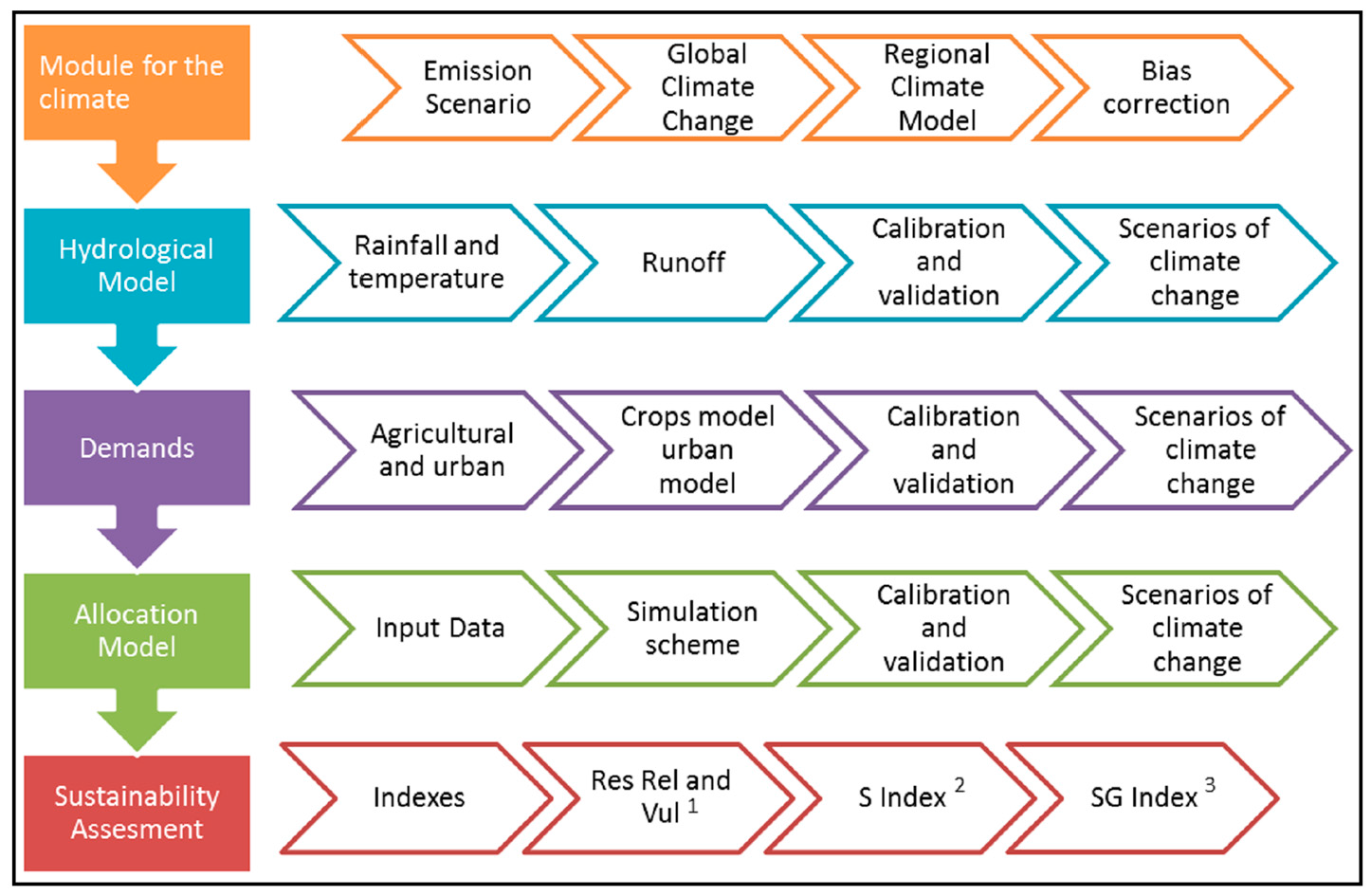
The assessment of methodologies to estimate the effects of climate change requires an IWRM approach, carried out through the use of a modeling chain composed of several simulation models. The first step corresponds to the climate analysis. This step is composed of the following elements in sequence: emission scenario, global climate model, regional climate model and bias correction. It analyzes temperature and precipitation changes in the studied area. The results from these analyses are used in the next step, which refers to the simulation of the hydrological cycle by using a rainfall-runoff model. This model allows us to predict the performance of the water resource system in the coming years in the studied area. The third step corresponds to the application of a water resource management model. This model includes the results obtained from the second step and also the estimation of the evolution of the agrarian and urban water supplies in all of the considered scenarios. The final results include the evaluation of several indices (
I,
SI, and
SG) in order to describe the performance of the system. These steps are described in detail in the next subsections and schematized in
Figure 1.
2.1. Climate Change Scenarios and Downscaling
Representative concentration pathways (RCPs) are the most recent climate change scenarios, which were developed via Community Integrated Assessment Modeling (IAMC), and are based on experiments in the literature for RCP 2.6, RCP 4.5, RCP 6.0, and RCP 8.5 [
25]. These scenarios include the anthropogenic greenhouse effect since pre-industrial years. Projections of rainfall and temperature are generated for atmosphere-ocean general circulation models (AOGCMs) [
26].
Regional climate models are responsible for downscaling rainfall and precipitation data from AOGCMs scenarios. The objective of downscaling is to adapt the results obtained from large-scale models into smaller scales in order to apply these data to impact studies. Statistical models and dynamical models represent the most common approaches for downscaling [
27]. Dynamical models for downscaling are as follows: HadCM3, RegCM, CRCM, RSM, MM5, and WRF [
28]. Statistical downscaling could be done with a weather generator (WG), and many WG have been proposed based on the Markov-chain model [
27].
From these results, high-resolution data of rainfall and temperature were generated based on weather stations and regionalized climate change scenarios RCP 4.5, RCP 6.0, and RCP 8.5. As in many other works related to climate change [
29], the method of inverse distance weighting (IDW) [
30] was performed in order to interpolate this information. After this, a linear bias-correction for mean and variance was applied for all stations with the objective of improving the accuracy of regional data [
31].
2.2. Development of the Hydrological Model
The hydrological cycle simulation was performed by using the Témez model [
32]. This is a monthly rainfall-runoff model composed of two storage tanks that allow surface runoff without the soil being fully saturated, along with a more realistic distribution of surplus between its water surface runoff and groundwater recharge [
33]. Its main advantage is the small number of parameters, in contrast to other models that have more [
34,
35] and whose estimation is very difficult to determine [
32]. The model has been incorporated into the EVALuación del recurso HIDrico (EVALHID) program (Valence, Spain) [
36], which is a module for the development of rainfall-runoff in complex basins integrated in AQUATOOL DSSS [
12]. It allows for the incorporation of other hydrological models, such as the Hydrologiska Byråns Vattenbalans-avdelning (HBV) model [
37] and the Sacramento model [
38], among others. After calibrating the four parameters for the Témez model, we incorporated the new climate change scenario variables and evaluated the differences in surface runoff and recharge.
2.3. Water Resource Management Model
IWRM was modeled with the AQUATOOL DSSS. It was developed by the Department of Water Resources of the Technical University of Valencia and it essentially allows us to create complex simulation allocation models that include surface, groundwater systems, and water quality [
12].
The SIMGES module (SIMulación de la GEStion) [
12] is a general model for the simulation of complex water resource systems, which can incorporate infrastructure elements or surface and groundwater storage included in the AQUIVAL module [
39]. In addition, it permits the creation of storage elements, transport, use and/or consumption, and elements of artificial recharge. The SIMGES module allows for the generation of a realistic topology based on rivers, aquifers, demand centers, reservoirs, and a realistic interaction between them [
40]. Based on the scheme and operating rules, the model uses an out-of-kilter optimization algorithm [
41] to determine flow solutions trying to satisfy different objectives for each month [
12,
42].
2.4. Demands Model
For the calculation of crop requirements, the methodology developed by the Food and Agriculture Organization for the United Nations (FAO) and the CROPWAT 8.0 software, was implemented [
43]. The panel recommended the adoption of the combined Penman-Monteith equation as a new standard to calculate reference evapotranspiration and suggested procedures for the estimation of the different parameters. The method overcomes the shortcomings of the previous FAO Penman model and provides more consistent values with actual water use [
43].
Urban demand was determined according to the methodology used by the Operator Agency Water and Wastewater of Morelia (OOAPAS), which considers the increase of population, the overcrowding index, the network coverage, the population served, and the losses in the system [
44].
2.5. Indices
The IWRM recently started studies integrating much of the information necessary for the analysis that involves both surface and groundwater elements; due to its complexity, it is common to evaluate the elements separately, and only a few studies include all of the elements of a real system [
19]. The IWRM approach introduces the climate impact as another variable that is involved in surface runoff, aquifers, environmental flow, supply to demands, and storage dams, among others. Therefore, it is necessary to evaluate the system as a conjunctive whole, where each element affects, in a different sense, the availability of water on each basin. For these reasons, it is necessary to develop a methodology to evaluate the availability of water from different points of view. The proposed indices focus on aquifers, surface runoff, environmental flow, supply to demands, and storage dams. These indices have been incorporated by reliability, resilience, and vulnerability, elements that are necessary to determine the sustainability index
and sustainability by groups
[
45].
2.5.1. Indices of the Integrated Water Resource Management (IWRM)
For the present study, we propose combining different indices in order to determine the effect of climate change on IWRM to provide detailed information of the different elements, as well as their interaction. Therefore, the results provide more global consequences of climate change and operational oversight in order to achieve the sustainability of the system itself. The indices in IWRM are only focused on part of the real system (e.g., as rainfall, surface runoff, aquifer recharge, and supply among others), and it is required to first evaluate them separately and then to integrate them.
The first index proposed is
, similar to the index
Ik proposed by Carrasco et al. [
17]. It concerns the supply to different demands (Equation (1)). The index is defined at a monthly scale by the relation between supplies and the amount of water required by demands along the simulation period.
where
is the monthly supplied water (hm
3/month).
is the demand of the basin (hm
3/month), and
is the month
. This index varies from 0 to 1. Values close to 1 indicate an acceptable supply to demand. By contrast, values close to 0 indicate that demand is not adequately supplied; the value of 1 indicates the full satisfaction and a value of zero indicates that there is not enough water to supply that demand.
The second proposed index
is the sum of the volume of the dam
at a given time
divided by the maximum volume
in the simulation period (Equation (2)). Values close to unity indicate that the dam is close to its maximum capacity and a value close to zero indicates periods of the worst droughts. It is also necessary to set a boundary in which to establish a desirable minimum volume in the dam, which will depend on each case study; for example, with specific operating rules associated with the system and the minimum conditions of operation.
The
index (Equation (3)) indicates the degree of pressure from the different demands on the aquifer and is defined as the total recharge to the aquifer
divided by the total demand from the aquifer
where
is the different demand
on the aquifer at month
, such as demand for urban, agricultural, or industrial use (hm
3/month). In the case of the
, the recharge of aquifer
for a month
is due to rain, infiltration of irrigation returns, and horizontal recharge from other aquifers, among others.
The fourth proposed index
indicates the availability of the surface resources (Equation (4)), which is the sum of the surface runoff in the simulation period
divided by the surface demand in the system
. This index is the inverse of water exploitation index (WEI) proposed by [
46]:
where
indicates the surface runoff in the whole system for the month
(hm
3/month), where
indicates the month in the simulation time.
refers to the surface demand system for a month
and demand
. Greater or equal to one value indicates that the system demands (hm
3/month) are lower than the surface runoff for a given year.
The index
indicates the volume of water flowing through the river (Equation (5)). It represents the ratio between the volume that flows through a river
(hm
3/month) and the environmental requirements
(hm
3/month).
where
is the number of stretches in the river.
The index
is complementary because it only indicates the supply to different demands.
is complementary and reflects the average conditions of the amount of water stored in dams during the simulation period. The rest of the indices include system conditions, (recharge demand in the aquifer, runoff demands, and environmental flow).
shows if the volume of water recharged is large enough to supply demands.
suggests if surface runoff volume is sufficient to supply the surface demands of the system in the natural regime. Finally,
shows if surface runoff is equal or greater than the environmental requirements. The importance of the indices depends on each individual case, since the method could be applied to any water resources system.
denotes the volume of each element (
Section 2.5.3). For each of the indices described we applied a determined sustainability index based on reliability resilience, as well as vulnerability (
Section 2.5.1) [
45,
47] in the case of sustainability by groups for the three last indices (
Table 1).
2.5.2. Reliability, Resilience, and Vulnerability
Hashimoto et al. [
48] proposed the criteria of reliability, resilience, and vulnerability with the challenge of analyzing different operating rules. Afterward, sustainability and relative sustainability [
45,
47] were proposed. These indicators have been applied in the evaluation of water resource systems and are two of the most popular [
15,
45,
49,
50,
51,
52]. We applied these criteria for the proposed indices (
Section 2.5.1).
Reliability (Equation (6)) measures the probability that each index
is satisfactory within a certain range [
47]. When deficits occur
we calculated the vulnerability [
45]. When the index
is less than one, it suggests that there is a deficit
. For
, it indicates that the volume is less than its minimum capacity of desirable operation
values less than this volume indicate that the dam was found in an unsatisfactory range
. For
, it shows that recharge is less than the demand
. For index
, deficit occurs when the surface runoff is lower than the demands on the system
.
denotes the volume when a stretch of river is less than the environmental requirements
.
where
refers to the reliability for the index
and
is the number of total simulations that, in this case, was simulated month by month.
Resilience measures the probability of a successful period followed by a period of failures [
53]. According to Hoque et al. [
54], it measures the rate of success in a system (Equation (7)). Values close to zero do not comply with the established criteria and values close to one indicate a greater number of situations of success.
where
is the resilience for index
,
is the month, and
is the number of times in which the index is less than one.
Vulnerability measures the magnitude or duration of a failure criterion (Equation (8)). This index also varies between zero and one [
45]. The average vulnerability was determined based on the index analyzed which, in all cases, refers to the average of the volume of the deficit (sum of deficits/number of times deficits occur) divided by the average volume of demand, dam, or environmental flow; these three changes in Equation (3) are a joint criteria for judgment
). The deficits are explained in the description of reliability
where
is the vulnerability of the five indices proposed (
Section 2.5.1); the first index
indicates the average water demand (hm
3/month); in the case of the dams (
),
is the minimum acceptable volume in the reservoirs (hm
3/month), whereas for index three
,
is the volume of aquifer demand (hm
3/month); for index
,
indicates the average water demand (hm
3/month); in the case of environmental flow
,
represents the environmental requirements (hm
3/month).
2.5.3. Sustainability Index
The sustainability index is one of the most popular approaches to analyze and compare different scenarios [
52]. Loucks [
47] proposed quantifying the sustainability of water resource systems using Equation (9), but only used the simple multiplication without the geometric mean. Sustainability varies between 0 and 1, and this index has an implicit weight; therefore, the weight of reliability, resilience, and vulnerability affects the sustainability index. Sandoval-Solis et al. [
45] proposed a variation that is the geometric mean of the different terms (Equation (9)). The advantage of the determination of
SI is that it is applied to different groups of elements of IWRM.
Sustainability by groups (Equation (10)) was divided into two components, sustainability of supply to demands
and sustainability by groups of indices
, which were based on the surface availability, pressure on the aquifer, and satisfaction of environmental requirements.
is the most relevant because it includes different elements. In order to evaluate the sustainability by groups (
) the following equation was used [
47]:
where
is the weight based on the volume of water demand,
is the sustainability, and
is sustainability by groups (
Table 1).
2.5.4. Summary of the Methodology
In brief, we describe the methodology through the following steps for preprocessing results:
First, based on calibrated and validated scheme in AQUATOOL DSSS for the years 1980–2009 (current scenario), evaluate the climate change scenarios (RCP 4.5 2015–2039, RCP 6.0 2015–2039, RCP 8.5 2015–2039, RCP 4.5 2075–2099, RCP 6.0 2075–2099, RCP 8.5 2075–2099) using the AQUATOOL DSSS.
Then, extract the results of demands, supplied water, recharge in the aquifer, storage dams, surface runoff, and environmental requirements for both the current and the climate change scenarios.
After that, determine the indices and sustainability indices through the following steps:
- 3.
Estimate the indices according to Equations (1)–(5).
- 4.
Calculate the reliability, resilience, vulnerability, and sustainability index through Equations (6)–(9).
- 5.
Estimate the weights of each sustainability index.
- 6.
Calculate the sustainability by groups (Equation (10)).
3. Case Study: Rio Grande Basin of Morelia, Mexico
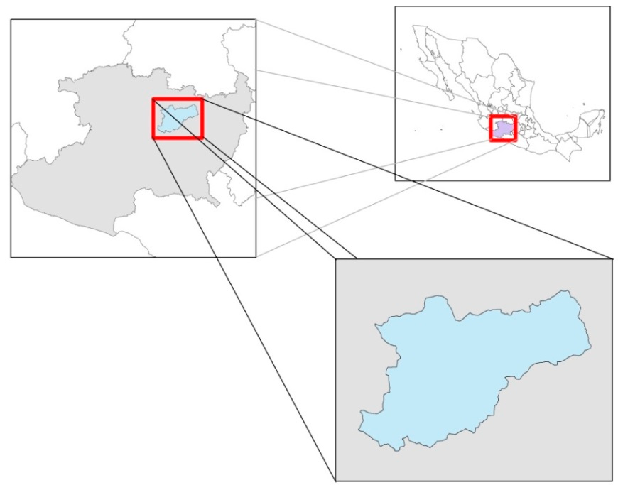
The basin of the Rio Grande of Morelia (
Figure 2) is located in Hydrological Region No. 12 B, as part of the sub-basin of Cuitzeo Lake. The studied area is located in the north-central portion of the state of Michoacán. It covers an area of approximately 1487 km
2 (Rio Grande and tributaries). The largest river supplies four Irrigation District (I.D.) Modules. Modules 1 and 2 are supplied by rivers and channels, and Modules 3 and 4 are supplied by surface and groundwater. The crops grown in the prevailing I.D. are as follows: Module 1, clover; in Module 2, corn; in Module 3, alfalfa, as well as corn; and in Module 4, wheat and corn.
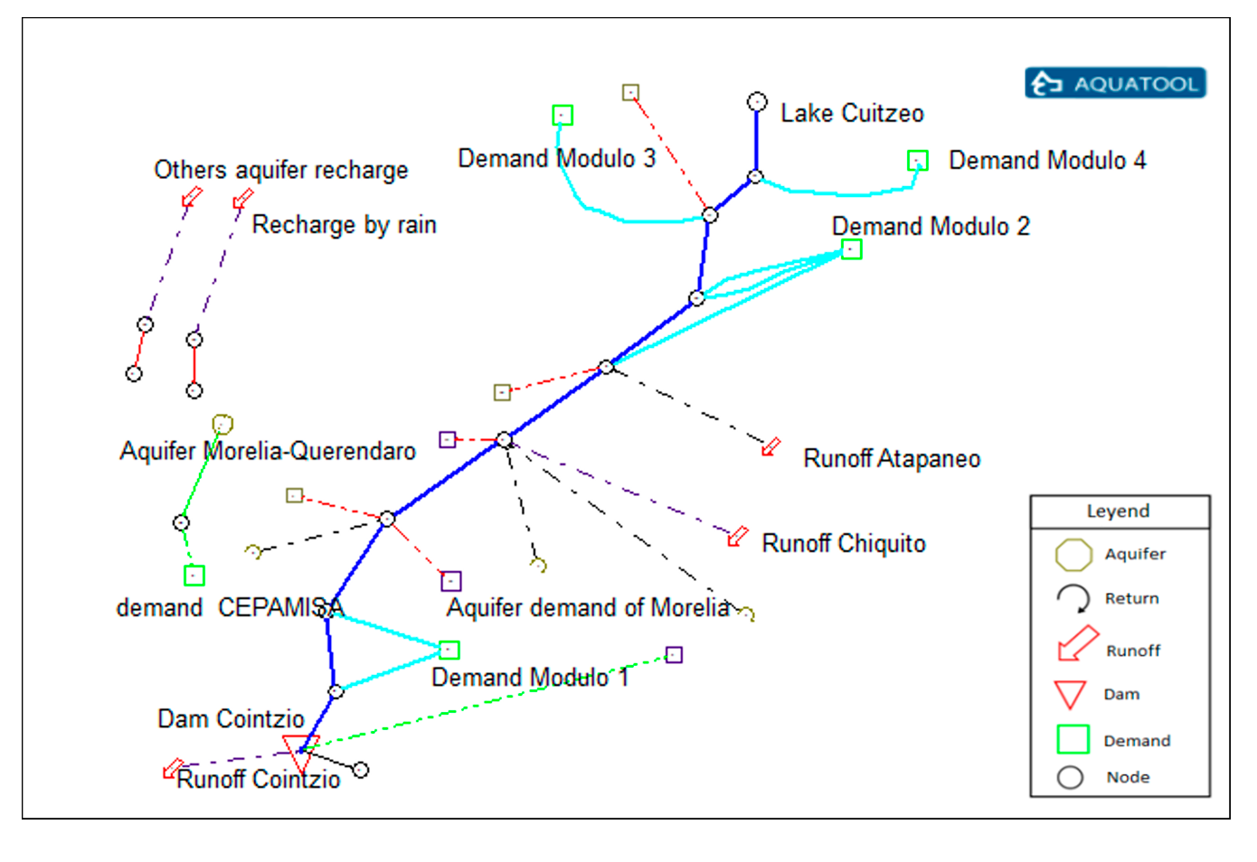
The Rio Grande is an endorheic basin and the principal surface runoff is the Rio Grande of Morelia. The Cointzio dam is located 11 km southwest of the city, the Mintzita reservoir is located 8 km southwest of the city, and Lake Cuitzeo is located 39 km north of the city. The increase in population is an important factor that causes greater water demand. Today, the entire volume of surface and groundwater in the basin is in use and, for that reason, it faces serious shortages in the near future. The Cointzio dam is mainly used to supply the urban demand for Morelia as well as I.D. 020 Morelia-Queréndaro. The wellspring Mintzita supplies the industrial demand of Crisoba Industrial, S.A. De C.V. The Morelia-Queréndaro aquifer supplies different demands, including urban demand for Morelia and Irrigation District Morelia-Queréndaro, and a group of demands which are considered together in the aquifer (
Figure 3). In this territory it is totally forbidden to pump and it is subject to the provisions of four decrees published in the Official Gazette in 1956, 1964, 1975, and 1987 [
55]. The main superficial demands are the urban demand of Morelia, and the four I.D. modules, 020 Morelia-Queréndaro, where the most important is Module 3, which represents 62% of the current demand.
For the climate change scenarios for the specific case of Mexico, the Mexican Network of Climate Modeling (CICESE, IMTA y CCA-UNAM), coordinated by the National Institute of Ecology and Climate Change (INECC), downscaled the resolution to half a degree (50 km × 50 km) of the 15 general circulation models (GCMs) of the Coupled Model Intercomparison Project Phase 5 (CMIP5) project. The National Institute of Ecology and Climate Change (INEEC) evaluated a multi-model ensemble of 15 GCMs for the near future (2015–2039) and by the end of the century (2075–2099). The multi-model ensemble that was generated [
28] was based on the methodology of the ensemble averaging reliability [
56], following a quality control-distributed CMIP5 [
57,
58].
Environmental flows were assessed according to Mexican Standard NMX-AA-159-SCFI-2012 [
59]. We determined the environmental flow for the current scenario and compared those flows with respect to climate change scenarios. We defined the ratio between the volume that flows through a river (climate change scenarios) and the environmental requirements (current scenario).
4 Results
4.1. Current Scenario
The simulation with SIMGES requires a previous calibration phase (1980–2009), which includes different elements like surface runoff, groundwater recharge, and urban and agricultural requirements (
Figure 3). The Cointzio dam regulates the surface runoff; this contributes to the Río Grande of Morelia, which is the main drainage basin, in its course towards the Cuitzeo Lake, which also supplies Irrigation District (I.D.) 020 Morelia Queréndaro and the city of Morelia. Urban demand is supplied by surface and groundwater resources.
In this paper, we focused on presenting the results of the indices, reliability, resilience, vulnerability, sustainability index, and sustainability by groups, and steps 3–6 from
Section 2.5.4. The results of the first index are presented below for the current scenario (1980–2009). Urban demand for Morelia has an index of 0.979 supplied by the aquifer (59.63%) and with surface runoff (38.36%). Demand Module 1 I.D. is supplied entirely by resources from the river without deficits, with
= 1.0; for Module 2,
0.975, supplied by rivers; for Module 3,
0.967, supplied by rivers (86.74%) and groundwater resources (10.02%); and Module 4, the rate is 0.983 with 96% supply by river and 2.43% from the aquifer; and in deep wells in Morelia, the index value is 1. For the system the indices equal the following; in the case of the Cointzio
the degree of pressure of the aquifer is
; for the supply to demands system,
; and the index of surface runoff
(
Table 2). We can observe the actual condition in the boundary of the system, i.e., the supply to demands is acceptable, similar to the degree of pressure of the aquifer
. In the case of the Cointzio dam
, the index is not close to one, but can supply to different demands, therefore exhibiting an acceptable value (for this study, we considered the 25% of the Cointzio dam according to operating rules of the system). Index
varies depending on the season, it is close to one for October–May, and the rest of the year decreases, especially in the first part of the river.
For Step 4 of the summary methodology, we calculated the reliability, resilience, and vulnerability for different indices. Furthermore we join the system indices, as well as the rate of supply to demand, and
and
are calculated. The reliability for the different demands
is between 0.572 and 1; the resilience is between 0.769 and 1, except in I.D. Module 2 (0.221); the vulnerability for all cases is around zero. The lowest sustainability index is
for I.D. Module 2 and the highest is
for I.D. Module 1. For indices
the reliability is less variable (0.684–1). Resilience is 0.351–1, and vulnerability is around zero. The lowest sustainability is
for
and
for
(
Table 3).
Steps 5 and 6 include the weight of each
and sustainability by group (
). Two
were studied; the first
for index
, and
in the case of indices
. We decided not to include
the Cointzio dam because of the variability in the year. For the current scenario,
, which is sustainable for the historic period; however, it presents some problems in terms of supply to demand. On the other hand,
(
Table 4) indicates an acceptable value for the system. The most important element for
SG is I.D. Module 3 (M3) with a weight of 0.392. For the system, the most important factor is the pumping of the aquifer with a weight of 0.538 (
Table 4).
4.2. Scenarios of Climate Change
For the analysis of climate change scenarios, periods of 25 years were established (2015–2039 and 2075–2099), in cycles or periods of 25 years. This periods were selected because the probability of occurrence of (CC) increases with time [
28]. The following six scenarios are evaluated. Scenarios of climate change are divided into RCP 4.5 2015–2039, RCP 4.5 2075–2099, RCP 6.0 2015–2039, RCP 6.0 2075–2099, RCP 8.5 2015–2039, and RCP 8.5 2075–2099. The results for the river basin indicate that temperatures will rise between 1.2 °C (4.5 RCP 2015–2039) and 4.5 °C (8.5 RCP 2075–2099) and decreases in precipitation between −11.8% (RCP 6.0 2015–2039) and −25.4% (8.5 RCP 2075–2099;
Table 5).
Regarding the volume of surface runoff, the most critical scenarios in the current century are RCP 6.0 2015–2019, with decreases from −23% and RCP 8.5 2070–2099 (−58.3%), with respect to the current period (179.2 hm
3/year). Recharge of the aquifer in the current scenario is 284.1 hm
3/year and this will be reduced in the most dramatic scenario −28% (8.5 RCP 2070–2099) and in the most optimistic conditions −11.4% (6.0 RCP 2015–2039;
Table 5).
Six climate change scenarios were evaluated by the module Irrigation District (24 scenarios). The current demand is 88.3 hm
3/year, which will increase to 95.6 (8.3%) hm
3/year in the most critical scenario RCP 8.5 2015–2039 and up 105.5 (19.6%) hm
3/year for RCP 8.5 2075–2099. For urban demand, the results indicate that, for the current scenario (82.1 hm
3/year), it will increase to 108 hm
3/year on average for the years 2015–2039 and 194.6 hm
3/year in 2075–2099 (
Table 5). This demand increases more than double due to the predicted rapid population growth in the city. This growth will also affect the Morelia-Queréndaro aquifer, causing decreases in the phreatic level.
4.3. Indices
For the case study, all indices, including CC, decrease in relation to the current scenario. For index
Morelia urban demand is mainly supplied by the aquifer and shows decreases in index
between 0.154 and 0.337, relative to the current scenario
. For RCP 8.5 2075–2099,
and for RCP 6.0 2015–2039
. Modules 1 and 2 will be most the affected in the I.D., which are supplied by the river.
for Module 1 and
for Module 2, for RCP 8.5 2075–2099. Module 3 is the least affected with an index and
for the same scenario. For the near future scenario, RCP 8.5 2015–2039 will be the most critical in the period with an index of
for Module 2, and Module 3 is, again, less affected in RCP 6.0 2015–2039, with an index of
. The full results are shown in
Table 6.
Index
reduced rapidly for climate change scenarios RCP 8.5, RCP 6.0, and RCP 4.5 in the period of 2015–2039, and is not able to supply to demands as index
for the three scenarios, and it fails to satisfactorily supply the different demands, according to the index
, presented before. For the RCP 8.5 scenario from 2075–2099 the value decreases very significantly until
. Therefore, the volume of the reservoir reaches its minimum capacity throughout this period (
Table 7).
The Morelia-Queréndaro aquifer is the most important because of its volume, which supplies the different demands. Therefore, as one of the vital elements of the system, the current state of the aquifer showed decreases in the phreatic level, mainly in the city of Morelia. The Morelia-Queréndaro aquifer supplies different and important demands such as Morelia, Module 3. For climate change scenarios, index
will be reduced between −10.24% (RCP 6.0 2015–2039) and −14.42% (8.5 RCP 2015–2039), indicating declines in the phreatic level of the aquifer, as well as lower supply to demands. Importantly, the operating rules for the system only allow extraction to a certain volume to avoid minor declines in the aquifer. For scenarios of the end of the century (
Table 7) the rate drops to
in the RCP 8.5 scenario,
for RCP 4.5, and
for RCP 6.0.
Demands and surface runoff are also evaluated by
The results indicate a reduction in the availability of the surface system with respect to the current scenario, where the supplies are guaranteed but, when including climate change scenarios (
Table 7), this will be reduced to less than −10% for the three scenarios in the years 2015–2039. At the end of the century, it will be affected more in RCP 6.0 2075–2099
and RCP 8.5 2075–2099
.
Regarding the surface runoff in the Rio Grande de Morelia, 12 sections were analyzed. They were selected when there are returns or any change in the volume streamflow. For climate change scenarios (
Table 7)
will be reduced in the near future to
(RCP 8.5 2015–2039), and for the distant future to
(RCP 8.5 2075–2099). This index is less critical than the others and only decreases by 0.059, with respect to the current scenario (
Table 7).
4.4. Sustainability Indices
Step 4 of the summary of the methodology calculates the reliability, resilience, vulnerability, and sustainability index. Sustainability, including CC, gets worse because all of the indices proposed decrease, hence the vulnerability is significant and the resilience, reliability, and sustainability are less than the current scenario. The sustainability index (
) in RCP 4.5, RCP 6.0, and RCP 8.5 scenarios (2015–2039) for the index
decreases due to reliability and resilience, which show the largest decrease, mainly in the most critical scenario (RCP 8.5). In the case of indices
, the decrease in reliability and resilience and the increase in vulnerability and index
are the most critical conditions and, therefore, lower the sustainability index. The full results are shown in
Table 8.
At the end of the century (2075–2099) in RCP 4.5, RCP 6.0, and RCP 8.5 scenarios, index
is the most affected by urban demand and I.D. Module 2 demand. The vulnerability module increases toward the most critical scenario (RCP 8.5) and decreases the reliability, resilience, and vulnerability. For the indexes
the results show the same behavior; the RCP 8.5 scenario is the most critical and the RCP 4.5 scenario is the most optimistic. Index
represents the worst changes due to CC for reliability, resilience, vulnerability, and the sustainability index; e.g., the elements in scenario RCP 4.5 2075–2099, with respect to RCP 8.5 2075–2099, decrease significantly (
Table 8).
For the most critical scenario, RCP 8.5 2075–2079, and for the index
, the reliability ranges from 0.281 (Morelia) to 0.674 (I.D. Module 3), resilience varies from 0.114 (Morelia) to 0.543 (I.D. Module 3), and vulnerability for all demands is less than 0.074 (I.D. Module 3). The
for
varies from 0.321 to 0.697. For the deep wells the sustainability index is zero because the pumping in the system is less than the demand and we decide not to include it in the table for all scenarios. For the indices
the reliability is near to zero (0.042–0.167), similar to resilience (0.043–0.2), the vulnerability increases between 0.286 and 0.694 and
decreases from 0.071 to 0.288.
is less sensible than the other indices and similar to
. Full results are present in
Table 8.
Step 5 calculates the weights of The including CC, depends on the sustainability index () and the weight of each index (); this weight changes for all scenarios due to the volume of the supply, demands, pumping, and streamflow variations in time for each CC scenario.
Finally, in step 6 of the summary of the methodology we estimated the
based on the weights of
. For the RCP 4.5 2015–2039 scenario,
(
Table 9), which is 0.3371 below the current scenario of the system
), thus, the index drastically declines in terms of system availability for this and other scenarios. The most optimistic scenario is RCP 6.0 2015–2039, where
SG1 = 0.539, which is a decrease of 0.335 over the current scenario. In the case of the most pessimistic scenario RCP 8.5 2015–2039,
(0.448) and
(0.351), less than in the current scenario (
Table 9).
Between the years 2075 and 2099, following the trend of even more worrisome declines, the index is between
(RCP 4.5) and
(RCP 8.5); these results indicate that the demand supply will be very poor. The decrease is similar to
(RCP 4.5 2075–2099). The RCP 8.5 scenario 2075–2099
predicts the worst system availability, supply to demand, surface runoff, dam volume, and phreatic level of the aquifer (
Table 9).
5. Discussion
The annual average surface runoff defines the availability in a water resource system. Less surface runoff and recharge were observed in all scenarios analyzed. Surface runoff decreased especially in the months with the highest surface runoff (July–October) by the end of the century (2075–2099) in all scenarios studied. Differences in annual distribution (important for monthly availability) between climate scenarios from the current scenario were observed, with the largest decrease in August.
Agricultural demand will be affected in this century by two main factors: increasing evapotranspiration and decreasing precipitation, which indicate stress on the crops. In the case of urban demand, it will be doubled this century due to continued population growth in the city.
All climate change scenarios show widespread declines in all indices indicating lower availability, surface runoff, supply to demands, volume in the reservoir, and widespread declines in the phreatic level of the aquifer. The most critical scenario is the RCP 8.5 2015–2039, the most optimistic scenario is the RCP 6.0 2015–2039, and the average scenario is the RCP 4.5 2015–2039; this is consistent with the estimation of temperature and precipitation [
60]. In the case of the scenarios for the years 2075–2099, the most critical is RCP 8.5, followed by RCP 6.0, and RCP 4.5 is the most optimistic.
Index
is more vulnerable to demands which are supplied by rivers than demands which are supplied by aquifers. The main reason for this, we surmise, is that we can pump more water to supply to demands but in the case of the river we cannot do it because we affect other demands. The Irrigation District is the most affected in this sense, and the second one is the urban demand of Morelia. Index
decreases for all scenarios, indicating the volume of the dam reaches minimum volumes. This index can be discussed because it depends on the month. It is normal that the volume of the dam will be low during dry seasons and, for rainy seasons, it increases significantly; thus, it is important to define which is the acceptable boundary on each dam. For the present study, we propose 25% of the maximum volume of the dam as acceptable. The decreases of index
are due to two factors. The first is less volume of recharge, and the second is because of the increasing demands (urban, I.D.). This index is the inverse to the WEI proposed for streamflow [
46], but
was proposed for the aquifer, and assumes that when the recharge is greater than demands is equal to 1 (
According to the case study, this index is one of the most important of the IWRM approach because it represents the major percentage of demands. Index
, similar to
, depends on the surface runoff and the surface demands, and this aspect is relevant because we can analyze separately the condition of surface demands and aquifer demands. The
index represents the cases that occur when the volume of water is less than the environmental flow. This aspect is important in IWRM because environmental flows establishes the minimum conditions of volume in a river, and the results indicate decreases less than other indices, considering the current scenario.
Climate change reduces availability, and affects the surface and groundwater system, therefore affecting all indices and, thus, SI and SG. The indices most affected by climate change and population increase are . for decreases mainly due to the deep wells that cannot supply to demands for any scenario, which increases the demand along with the different scenarios analyzed. For indices , decreases primarily due to , because it presents greater in the system (RCP 4.5 and RCP 6.0). For the RCP 8.5 scenario, vulnerability increases considerably in , decreasing in reliability and resilience ; for these reasons serious problems of availability of water resources are expected.
The complementary indices developed in this study are focused on supply to demands and dam volume (); principal indices for the system are . These indices can be applied for current and future models of IWRM and from the particular point of view of each index. However, some methodological aspects chosen in this study limit the results of this paper. Firstly, it is noteworthy to highlight the information for the modeling of the IWRM. The available information could not represent the exact reality of the complex system (e.g., precipitation, temperature, water demands, and storage dams, among others). Secondly, the water availability is conditioned by the operating rules assumed for each demand. In the case of the agricultural demand, CROPWAT model does not simulate the phenologic stages of crops. Thus, a crop coefficient that constrains the model is necessary. Thirdly, the uncertainty associated with the scenarios of climate change (RCPs) and downscaling is important. These scenarios describe different ways of development in the emission of greenhouses gases and should not be seen as a policy descriptive.
All the assumptions used in the IWRM affect the results of the indices. For our case study, we assumed that the urban demand has priority above agricultural demand. For the climate change scenarios, we supposed the same operating rules as those in the current scenario. The use of a monthly scale simplifies the number of parameters in IWRM and CC. Based on this simplification; we are ignoring water scarcity at daily scale (SI, SG, Res, Rel, and Vul). The present approach focuses on the identification of existing or expected problems of water scarcity at monthly scale. However, the use of daily scale increases the number of parameters in IWRM as well as uncertainty.
6. Conclusions
Climate change will produce changes in temperature, precipitation, surface runoff, recharge, reserves, deficits in supply to demands, increased pumping, and increased vulnerability. Through the building of quantitative climate change scenarios, decision-makers can prioritize adaptation actions to prepare society for a different climate. In the present study, we have successfully developed various indices for IWRM with a holistic approach. The indices developed are applicable to any IWRM. Researchers can also use any combination of SI and SG, e.g., we can evaluate the surface system or, if we desire only to determine the supply to demand. This approach was conceived as a complement of the decision support system. The use of this approach gives us the possibility to identify vulnerability and sustainability in IWRM. In cases of complex water resource systems, indices are also useful to make different analyses and summaries. Furthermore, our approach is useful for comparative studies of the indices and sustainability.
The effect of climate change for the case study mainly affects the indices , . In addition to climate change, the urban population increase plays an important role in reducing these indices. shows the supply to demand is compromised (efficiency plays an important role in this factor). In addition, the volume of the dam is critical and extractions are far greater than the aquifer recharge . In the case of indices , the decrease is less important. does not decrease significantly, but the supply to demands indicates that a large amount of water is lost in channels and rivers. Although the operating rules enable the supply of demands and the use of available water, the surface runoff is lower than the environmental flow (). By the end of the century, it will be difficult to achieve the in the study area, and it is vital to take necessary measures to recover and adapt to climate change.
In general, a complex system is affected by different factors; less precipitation and high temperatures are the main factors for water availability. Small changes will affect any water resource system. As we have seen in this paper, the implications of CC are less surface runoff, volume of dams, volume in rivers, and increases of demands (urban and agricultural); thus, major risks of drought. In a complex system, a particular decision is not necessarily the solution to the problems of the system. It is important to make decisions based on the development of scenarios and methodologies, as presented in this article. For the effects of climate change, we need to consider operating rules and infrastructure development.
The main limitation of the present study is the lack of information provided by authorities and decision makers. On the other hand, the uncertainty associated with IWRM and climate change. This approach could be useful for decision-makers and water managers, especially because the indices and sustainability give us general and particular conditions of the system, and they are relatively easy to determine.
In the present work, we learned that it is important to see the availability of water from a general point of view, and it is necessary to consider all interactions of integrated water resources and management, as well as consider the infrastructure and operating rules of a complex system. With respect to climate change, at first sight it would seem that the effect of CC is small (in terms of surface runoff and environmental flow, among others), but the effects are magnified when we evaluate the IWRM and different indices. It is very important to learn about the study area and to have as much information as possible.


 and
and 

