Multiobjective Automatic Parameter Calibration of a Hydrological Model

Abstract

This study proposes variable balancing approaches for the exploration (diversification) and exploitation (intensification) of the non-dominated sorting genetic algorithm-II (NSGA-II) with simulated binary crossover (SBX) and polynomial mutation (PM) in the multiobjective automatic parameter calibration of a lumped hydrological model, the HYMOD model. Two objectives—minimizing the percent bias and minimizing three peak flow differences—are considered in the calibration of the six parameters of the model. The proposed balancing approaches, which migrate the focus between exploration and exploitation over generations by varying the crossover and mutation distribution indices of SBX and PM, respectively, are compared with traditional static balancing approaches (the two dices value is fixed during optimization) in a benchmark hydrological calibration problem for the Leaf River (1950 km²) near Collins, Mississippi. Three performance metrics—solution quality, spacing, and convergence—are used to quantify and compare the quality of the Pareto solutions obtained by the two different balancing approaches. The variable balancing approaches that migrate the focus of exploration and exploitation differently for SBX and PM outperformed other methods.

1. Introduction

A rainfall–runoff (RR) model is a mathematical model used to describe the RR process of a watershed, which generally produces a surface runoff hydrograph (output) using a hyetograph (input) [1]. The RR model is calibrated: (1) for estimating the model structure and parameters that enable the model to closely match the behavior of the real system it represents; and (2) for estimating model uncertainties. A hydrologist wants to develop a hydrological model with not only high accuracy (i.e., the former case for minimizing a bias) and but also high precision (i.e., the latter case for a reliable performance).

During the past two decades, the development and calibration of RR models have been the focus of hydrological research [2,3]. Various RR models have been developed and are classified into lumped and distributed models. The former is based on the assumption that the entire basin has a homogeneous hydrological characteristic, whereas the latter divides the basin into elementary unit areas resembling a grid network to consider the spatial variability of the basin characteristics. The Sacramento Soil Moisture Accounting (SAC-SMA) model is an example of a lumped model, whereas the Systeme Hydrologique Européen-Transport (SHETRAN) [4] is a distributed model.

RR models never perfectly represent an actual system of interest, and the data used for calibration always contain measurement errors [5]. Although the main focus of hydrological research has been the development of automatic parameter calibration approaches, efforts have also been made to assess parameter uncertainty in RR models to quantify the inability of the model to produce precise and accurate results [2,5,6,7,8,9,10,11]. The present study focuses on the development of efficient and effective automatic parameter calibration methods.

The governing equations of RR models are used to define the RR processes, which consist of model parameters and variables. Traditionally, a manual approach has been applied in which a hydrologist estimates the value of the model parameters through a trial-and-error process in which the model matches the behavior of the actual system it represents [2]. The hydrologist’s experience and knowledge of the model (e.g., the model structure and sensitivity of model parameters) are key factors for the success of the model calibration in this approach. However, there is no guarantee that the hydrologist will find the best parameter set yielding the highest accuracy of the RR model through these time-consuming efforts because the optimal parameter calibration problem is highly nonlinear, multimodal, and nonconvex [12] for which a simple gradient-based technique cannot be used.

To overcome the limitation of the manual approach in the speed and reliability of the RR model calibration, an automatic, computer-based approach has been widely used during the last two decades [3]. Generally, an RR model is linked to stochastic optimization algorithms to evaluate the fitness of potential parameter sets and to identify the optimal parameter set resulting in the best accuracy for the model [13]. These algorithms include simulated annealing (SA) [14], genetic algorithm (GA) [15,16], particle swarm optimization (PSO) [17], harmony search (HS) [18], and shuffled complex evolution-University of Arizona (SCE-UA) [12]. The most popular measure of the fit of the model is the mean-square-error (MSE) estimator [2]. By using the automatic calibration method, the solution space can be explored in less time than that taken when using the manual approach.

Various model accuracy measures have been introduced to consider the different aspects of model accuracy. For example, use of maximum absolute error (MAE) focuses on the robustness of the model accuracy to minimize the worst deviation between the observed and simulated values [19,20,21,22,23]. The peak flow difference can generally be considered in the RR model for hydraulic structure design [19,20,21,22,23,24,25]. Therefore, a pair of competing model accuracy measures can exist among various measures. During the model calibration process, hydrologists often observe that increasing a model accuracy measure (e.g., the mass balance measure) cannot be achieved without sacrificing or decreasing another measure (e.g., the peak difference). This phenomenon has triggered the advent of multiobjective automatic model calibration models [2,10], which explore the trade-off in the relationship among two or three competing model accuracy measures.

Efstratiadis and Koutsoyiannis [26] provided a thorough review and summarized the critical issues in multiobjective calibration. They classified multiobjective calibration studies into aggregate and pure Pareto approaches. The former combines multiple objectives into a single objective by weighting them, whereas the latter identifies multiobjective optimal solutions (i.e., the Pareto optimal solution) by simultaneously seeking multiple objectives. Recently, calibration methodologies used specifically for pure multiobjective schemes have been introduced. Asadzadeh et al. [27] proposed a selection measure known as convex hull control (CHC) for solving a multiobjective calibration problem with a known and approximated convex Pareto solution.

Zhang et al. [28] performed sensitivity analysis of the parameters of the non-dominated sorting genetic algorithm-II (NSGA-II) [29] on the accuracy of a distributed hydrological model known as Systeme Hydrologique Européen-Transport (SHETRAN) [4,30,31,32,33,34,35,36]. Simulated binary crossover (SBX) [37] and polynomial mutation (PM) [38] were used for the crossover and mutation, respectively, of three NSGA-II algorithms: the original NSGA-II, the reference point-based-NSGA-II (R-NSGA-II) [39], and the extension ER-NSGA-II [40]. The root-mean-square error (RMSE) and logarithmically transformed RMSE (LOGE) between the observed and simulated hourly discharges were minimized simultaneously. Three combinations of crossover and mutation distribution indices (C_DI and M_DI, respectively), the parameters of SBX and PM, respectively, with values of (0.5, 0.5), (2.0, 0.5), and (20, 20), which were kept constant during optimization were applied. C_DI and M_DI control the closeness of the children solutions to the parent solutions in the crossover and mutation, respectively. Higher parameter values (e.g., C_DI = 20) result in children solutions that are more similar to the parent solutions, which are assigned more weight on exploitation.

Zhang et al. [28] assumed that the algorithm’s balance between exploration (diversification) and exploitation (intensification) did not change over generations, which is a static approach. The former is defined as the algorithm’s ability to search wide areas of the solution space (e.g., the random search of HS), and the latter refines the neighborhood of previously found promising areas in solution space (e.g., the crossover of GA). However, some studies reported that the balance should be variable to guarantee the best performance [41,42,43] because the effectiveness of wide search and fine-tuning depends on the optimization phase. Cuevas et al. [44] stated that a common strategy for balancing exploration and exploitation is to start with exploration and then gradually increase exploitation as good fitness points are identified. It would be a better strategy in the automatic calibration of a hydrological model to focus on searching various parameter sets broadly in the early optimization phase and to give more weight to fine-tuning the solutions found in the latter phase.

This study introduces variable balancing approaches for the exploration and exploitation of the NSGA-II with SBX and PM in the multiobjective automatic parameter calibration of a lumped hydrological model, the HYMOD model. The proposed balancing approaches, which migrate the focus between exploration and exploitation over generations by varying the crossover and mutation distribution indices, C_DI and M_DI, respectively, were compared to traditional static balancing approaches (the two dices value is fixed during optimization) in a benchmark hydrological calibration problem for the Leaf River (1950 km²) near Collins, Mississippi. Three performance metrics, solution quality, spacing, and convergence, were used to quantitatively compare the performance of the two different balancing approaches.

2. Methodology

This study compared static and variable balancing approaches for the NSGA-II by using SBX and PM operators in the multiobjective automatic calibration of a lumped RR model, the HYMOD model. Two types of parameters are used throughout the study: algorithm parameters (e.g., crossover rate, C_DI, and M_DI) and model parameters (HYMOD model parameters). An improved version of the HYMOD model was used to simulate the RR process of the Leaf River basin located north of Collins, Mississippi. First, the correlation among various model accuracy indicators (MAIs) was inspected by visual inspection, linear regression, and Pearson correlation analysis to select two competing objectives to be minimized in the calibration. In this study, the trade-off relationship between percent bias (PB) and the sum of three peak flow differences (TPFD) was explored by using the static and variable balancing approaches. The performance measures, solution quality, spacing, and convergence [45] of the Pareto optimal solutions were quantified to identify the best balancing strategy. The following sections describe the objective selection process, the multiobjective calibration model, NSGA-II, SBX, PM, performance metrics, and the improved HYMOD model.

2.1. Objective Selection Process

The accuracy of the RR model was evaluated by comparing the observed and simulated discharge values at specific points in the basin. The model parameters were calibrated to minimize the model error. The prediction always contains errors (i.e., deviations from the observed value) that are jointly influenced by: (1) measurement error; (2) inappropriate representation of the actual system; and (3) the lack of basin information for model development and parameter calibration [26].

Various model accuracy measures have been formulated and used for automatic calibration of RR models.

Table 1. Model accuracy indicators (MAIs) and their formulations.

Name (Abbreviation)	Formulation
Total Mean Squared Error (TMSE)	$\frac{1}{n}{\displaystyle {\displaystyle \sum }_{t=1}^n}{(o_t-s_t(\mathsf{\theta }))}^2$
Root Mean Squared Error (RMSE)	$\sqrt{\frac{1}{n}{\displaystyle {\displaystyle \sum }_{t=1}^n}{(o_t-s_t(\mathsf{\theta }))}^2}$
Nash–Sutcliffe Measure (NSF)	$1-\frac{\frac{1}{n}{{\displaystyle \sum }}_{t=1}^n{(o_t-s_t(\mathsf{\theta }))}^2}{\frac{1}{n}{{\displaystyle \sum }}_{t=1}^n{(o_t-\overline{o})}^2}$
Absolute Peak Difference (APD)	$\left|\underset{1\le t\le n}{\max }\{o_t\}-\underset{1\le t\le n}{\max }\{s_t(\mathsf{\theta })\}\right|$
Percent Bias (PB)	$100\times \left|\frac{\frac{1}{n}{{\displaystyle \sum }}_{t=1}^n{o}_t-\frac{1}{n}{{\displaystyle \sum }}_{t=1}^n{s}_t(\mathsf{\theta })}{\frac{1}{n}{{\displaystyle \sum }}_{t=1}^n{o}_t}\right|$
Mean Absolute Error (MAE)	$\frac{1}{n}{\displaystyle {\displaystyle \sum }_{t=1}^n}\left|o_t-s_t(\mathsf{\theta }\right|$
Maximum Absolute Error (MAE)	$\underset{1\le t\le n}{\max }\left|o_t-s_t(\mathsf{\theta })\right|$
Three Peak Flow Difference (TPFD)	${\displaystyle {\displaystyle \sum }_{t\in T_p}}\left|o_t-s_t(\mathsf{\theta })\right|$

Notes: $o_t$ is the observed streamflow at time interval t (t = 1, …, n); $s_t(\mathsf{\theta })$ represents the simulated streamflow at time t using the parameter values $\mathsf{\theta }$; $\overline{o}$ is the mean value of the observed streamflows during the period t = 1 to n; and T_p is a set of times at which the three largest streamflows occurred at the observed value.

summarizes several MAIs used by the National Weather Service for calibration of the Sacramento soil moisture accounting (SAC-SMA) model and MSE-based measures widely used in the domain of hydrological model calibration. Different measures represent different aspects of model error. For example, an MSE measure is appropriate when measurement errors are uncorrelated and more weights should be given to minimizing error at high flows. In contrast, the sum of peak differences is considered when an RR model is used for flood management when peak discharge is the main concern. Therefore, the appropriate model error measure should be carefully selected and used for effective model parameter calibration.

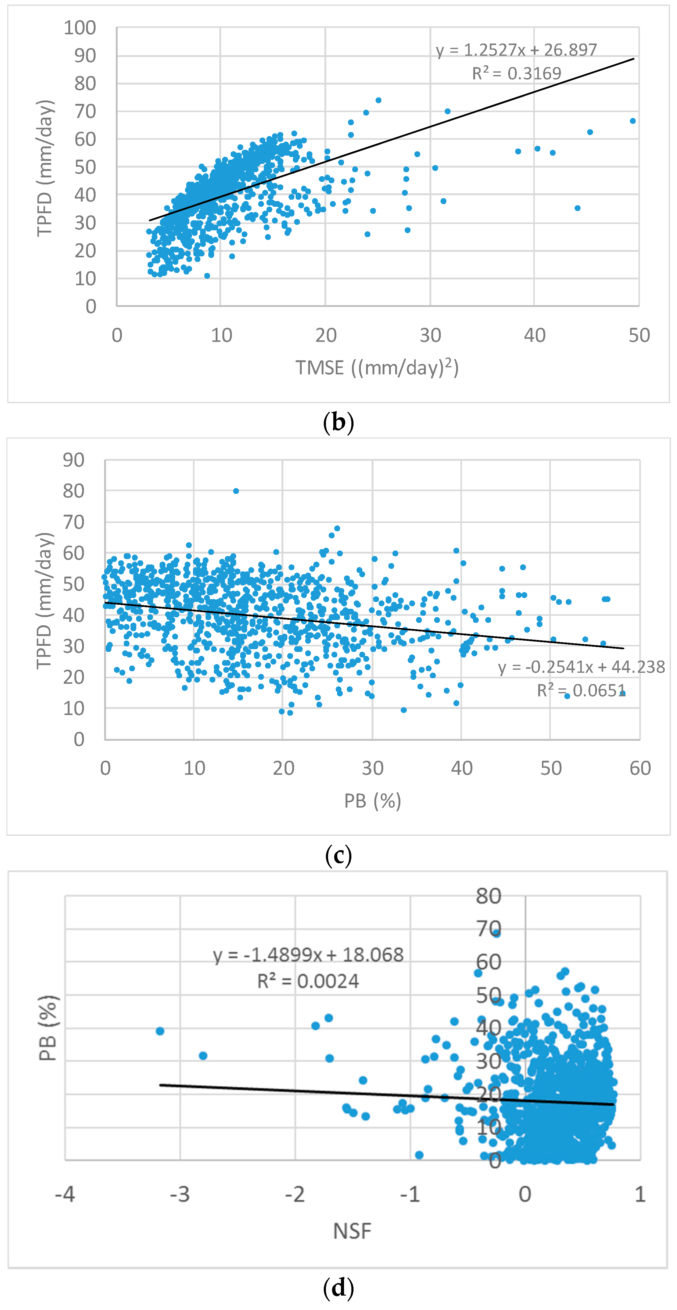
In order to construct a multiobjective automatic parameter calibration model, two competing MAIs should be identified. The two correlated indicators should not be simultaneously considered in the model because minimizing/maximizing one indicator would have the same effect on the other indicator. To that end, uniform random sampling within the upper and lower bounds of parameters, which is determined by physical reasonability, engineering knowledge, and Monte Carlo simulations (MCS) generates random parameter sets. A simulated hydrograph is obtained from the RR simulation using each generated parameter set for which the MAIs in Table 1 are calculated. Finally, the scatter plot of each pair of the MAIs in Table 1 and its linear regression line are drawn and inspected to detect the potential correlation.

2.2. Multiobjective Automatic Parameter Calibration Model

The two objectives selected from the objective selection process were optimized in the multiobjective automatic parameter calibration model of the hydrological model. Most MSE-type objectives are to be minimized, whereas a few accuracy measures are to be maximized (e.g., the Nash–Sutcliffe measure (NSF)). The decision variables of the model are the parameters (θ) of the hydrological model. The observed dataset of flow discharge was selected and provided to the model for fitting the simulated results. Therefore, the multiobjective parameter calibration model was formulated as

$$\{\begin{array}{l}\mathrm{Minimize} f_1=\mathrm{MAI}1(\mathsf{\theta })\\ \mathrm{Minimize} f_2=\mathrm{MAI}2(\mathsf{\theta })\end{array}, \mathsf{\theta }\in \mathsf{\Theta },$$

(1)

where MAI1 and MAI2 are the first and second different MAIs calculated given the model parameter θ, respectively; and Θ is the feasible parameter space defined by the minimum and maximum values of each parameter, assuming that the two objectives are to be minimized.

The two objectives were simultaneously optimized; they were not aggregated in this study. In the field of hydrological model calibration, the NSGA-II, Multiobjective Complex Evolution (MOCOM) algorithm and the Multiobjective Shuffled Complex Evolution Metropolis (MOSCEM) algorithm are widely used [8,46,47,48,49,50,51,52,53,54,55,56,57,58,59]. A set of Pareto optimal solutions (non-dominated parameter sets) was obtained from the model. Then, a best-compromise parameter set is identified and suggested among multiple Pareto optimal parameter sets based chiefly on the user’s judgment according to the analysis of the shape of the Pareto front.

2.3. NSGA-II with SBX and PM

This study used NSGA-II to find the Pareto optimal parameter sets in the multiobjective calibration model introduced in the previous section. The main mechanisms of NSGA-II compared with other multiobjective metaheuristic algorithms are the non-dominated ranking and consideration of crowding distance [29]. That is, a solution distant to others in the solution space and dominating other solutions with respect to fitness is more likely to survive to the next generation. Details of NSGA-II have been reported by Deb et al. [29].

This study employed SBX and PM operators for the crossover and mutation, respectively, of NSGA-II to improve the search power. It should be noted that the occurrences of the crossover and mutation operations are complementary, and their frequency is controlled by the crossover rate (Crate). Therefore, if the Crate is 0.9, the rate of mutation is 0.1. The SBX and PM operators control the spread of the children solutions compared with the selected parent solutions by C_DI $\in (0,+\infty )$ and M_DI $\in (0,+\infty )$. Therefore, the best strategy for the control of C_DI and M_DI should be identified and used to obtain the best effectiveness and efficiency of NSGA-II with SBX and PM.

The SBX operator produces two children solutions $x_i^{1,j+1}$ and $x_i^{2,j+1}$ from the two selected parent solutions $x_i^{1,j}$ and $x_i^{2,j}$ by using polynomial probability distributions

$$\mathsf{\epsilon }({\mathsf{\beta }}_i)=\{\begin{array}{c}0.5({\mathrm{C}}_{\mathrm{DI}}+1){\mathsf{\beta }}_i^{{\mathrm{C}}_{\mathrm{DI}}}, \mathrm{if} {\mathsf{\beta }}_i\le 1\\ 0.5({\mathrm{C}}_{\mathrm{DI}}+1)\frac{1}{{\mathsf{\beta }}_i^{{\mathrm{C}}_{\mathrm{DI}}+2}}, \mathrm{otherwise}\end{array},$$

(2)

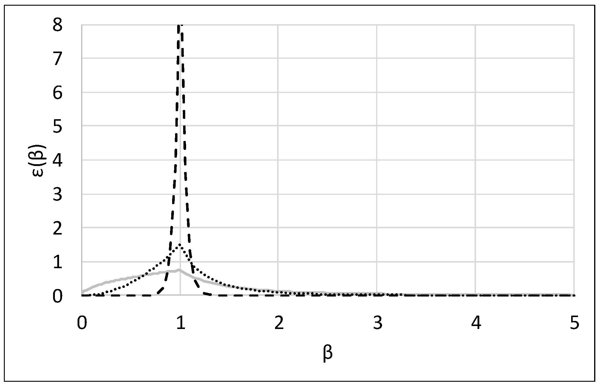
where ${\mathsf{\beta }}_i=\{\begin{array}{c}{(2u_i)}^{1/({\mathrm{C}}_{\mathrm{DI}}+1)}, \mathrm{if} u_i\le 0.5\\ {(\frac{1}{2(1-u_i)})}^{1/({\mathrm{C}}_{\mathrm{DI}}+1)}, \mathrm{otherwise}\end{array}$ which can be obtained by inverse transform sampling with a randomly generated number $u_i\in (0,1)$, and $\mathsf{\epsilon }$ is a probability function. As indicated in Figure 1, large values of C_DI result in a high probability of creating children solutions close to the parent solutions. Then, the children solutions are derived from the equations below:

$$x_i^{1,j+1}=0.5\left[(1+{\mathsf{\beta }}_i)x_i^{1,j}+(1-{\mathsf{\beta }}_i)x_i^{2,j}\right],$$

(3)

$$x_i^{2,j+1}=0.5\left[(1-{\mathsf{\beta }}_i)x_i^{1,j}+(1+{\mathsf{\beta }}_i)x_i^{2,j}\right].$$

(4)

The PM operator creates the child solution $x_i^{3,j+1}$ from the parent solution $x_i^{3,j}$ by using the polynomial probability distribution:

$$\mathsf{ϵ}({\mathsf{\delta }}_i)=0.5({\mathrm{M}}_{\mathrm{DI}}+1){(1-\left|{\mathsf{\delta }}_i\right|)}^{{\mathrm{M}}_{\mathrm{DI}}},$$

(5)

where ${\mathsf{\delta }}_i=\{\begin{array}{c}{(2r_i)}^{1/({\mathrm{M}}_{\mathrm{DI}}+1)}-1 \mathrm{if} r_i\le 0.5\\ 1-{\left|2(1-r_i)\right|}^{1/({\mathrm{M}}_{\mathrm{DI}}+1)}, \mathrm{otherwise}\end{array}$ and $\mathsf{ϵ}$ is a probability distribution function.

The child solution is then produced by the equation

$$x_i^{3,j+1}=x_i^{3,j}+(x_i^{UB}-x_i^{LB}){\delta }_i,$$

(6)

where $x_i^{UB}$ and $x_i^{LB}$ are the upper and lower bounds of the i^th decision variable, respectively.

Five parameters are used in NSGA-II with SBX and PM operators that affect the algorithm performance: the number of generations (NGEN), the number of populations (NPOP), Crate, C_DI, and M_DI.

2.4. Variable Exploration and Exploitation Balancing Approaches

The success of the metaheuristic optimization algorithm depends on the balance between the algorithm’s exploration (diversification) and exploitation (intensification) capability [44,60,61,62,63]. This study proposes variable changing methods for the C_DI and M_DI of SBX and PM, respectively. Using higher parameter values (e.g., C_DI = 20) assigns more weight to exploitation, whereas smaller parameter values (e.g., C_DI = 0.5) emphasize exploration (Figure 1).

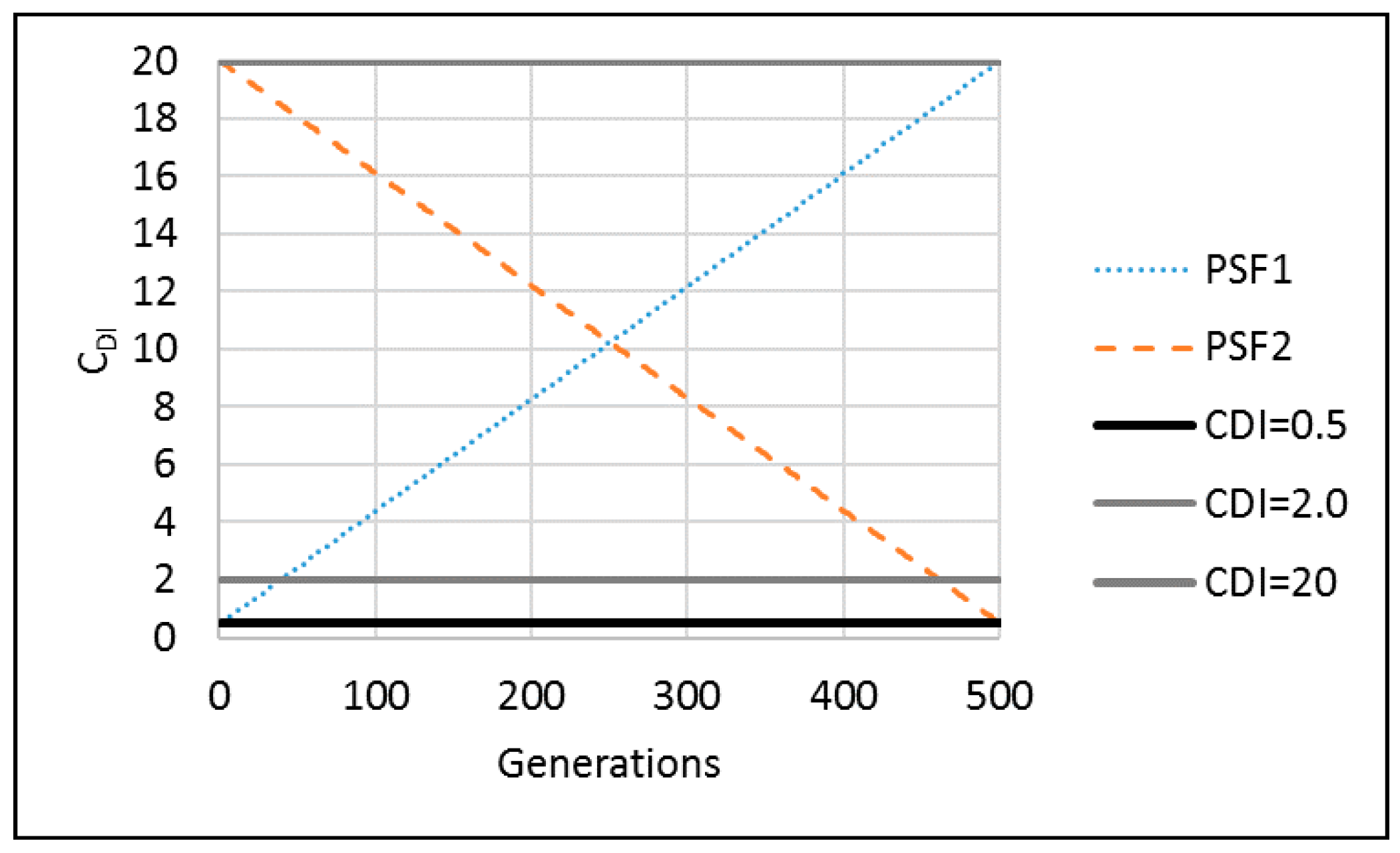
We can vary the balance between exploration and exploitation over generations by changing the C_DI and M_DI values. An example of the variable balancing approach is the so-called parameter-setting-free (PSF) method, which has been used by a few researchers in the field of applied mathematics for removing the burden on the user in selecting algorithm parameters [41,42,43].

Two respective representative PSF methods increase the algorithm parameter value from its minimum to maximum (PSF1) and decrease the algorithm parameter value from its maximum to its minimum (PSF2) (Figure 2). Therefore, the algorithm parameter at the generation igen, p_igen (e.g., p = C_DI or M_DI), is calculated as

$$\mathrm{PSF}1: p_{igen}=p_{\min }+\frac{p_{\max }-p_{\min }}{NGEN-1}(igen-1)$$

(7)

$$\mathrm{PSF}2: p_{igen}=p_{\max }-\frac{p_{\max }-p_{\min }}{NGEN-1}(igen-1),$$

(8)

where p_min and p_max are the minimum and maximum value of the algorithm parameter p, respectively. Four different variable balancing approaches for exploration and exploitation are generated from the combination of PSF1 and PSF2 for C_DI and M_DI. Therefore, Approach 1 uses PSF1 for both C_DI and M_DI, whereas Approach 2 applies PSF2 for both indices. In contrast, Approach 3 uses PSF1 for C_DI and PSF2 for M_DI, and Approach 4 applies PSF2 for C_DI and PSF1 for M_DI.

2.5. Performance Metrics

In order to compare the Pareto optimal solutions obtained from different approaches, three performance metrics were used: solution quality metric (SQM), spacing metric (SPM), and convergence metric (COM). The original SQM and COM were introduced by Wang et al. [64] and Kollat and Reed [65], respectively. SPM was originally proposed by Zheng et al. [45] for measuring run-time performance of multiobjective algorithms, which was modified in this study for the evaluation of the final Pareto solutions.

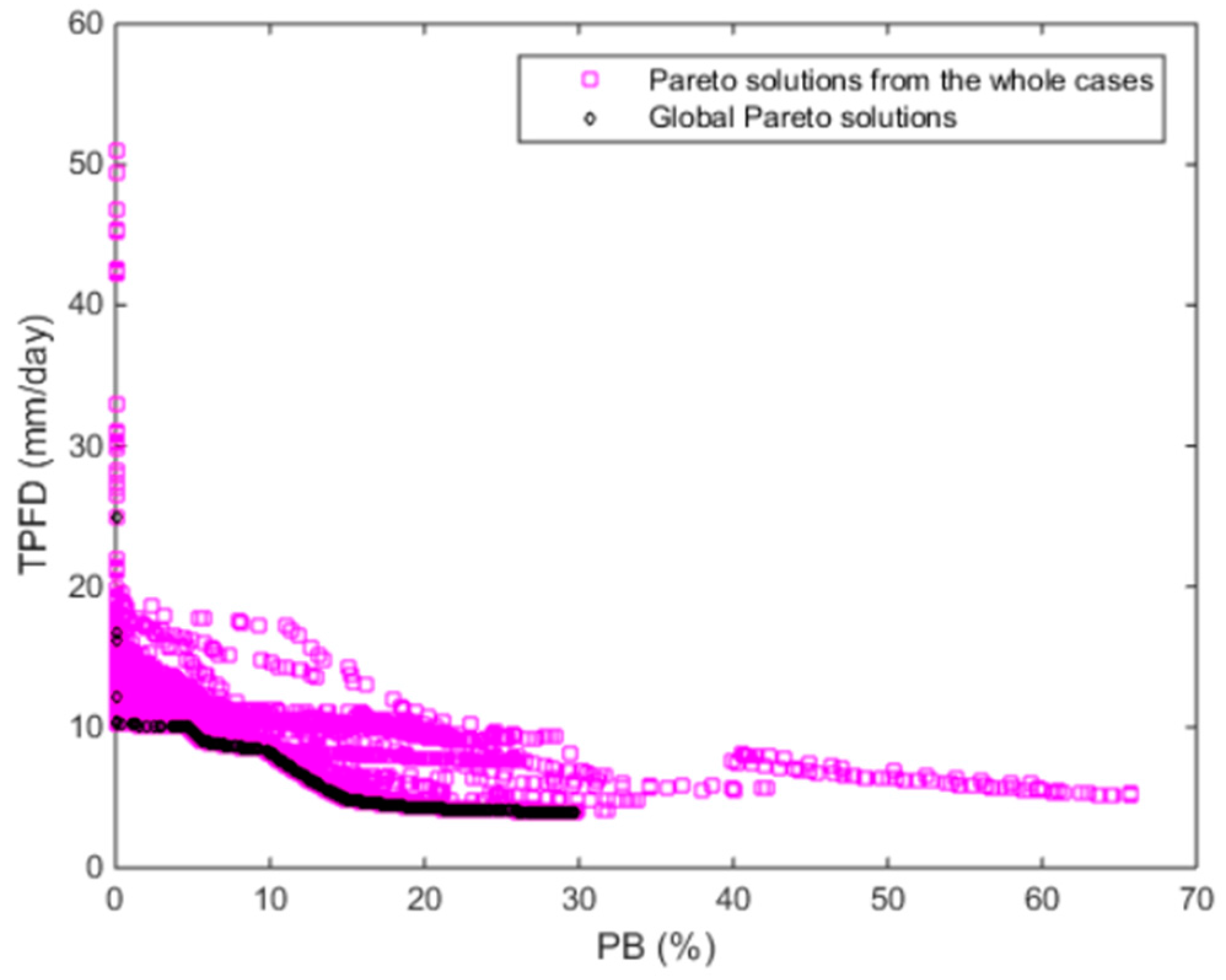
SQM quantifies an algorithm’s ability to find non-dominated solutions. The steps for calculating SQM are briefly described here. The final optimal Pareto solutions of all algorithms (all approaches or cases) are gathered to identify the global non-dominated solutions, also referred to as the global Pareto solution or the global Pareto front, Z*. The SQM of a case is equal to the number of non-dominated solutions found by the case in Z*.

Deb et al. [29] considered crowding distance to be an important factor for the selection of the children population so that NSGA-II would develop a wide-spread Pareto front, which is favored with respect to the final solution diversity and exploration [66]. The Pareto front with a wide range of objective function values means that the decision maker can choose from more parameter set alternatives. SPM quantifies the extent of the Pareto front relative to the Pareto front Z* as

$$\mathrm{SPM}=\frac{\underset{i,j=1, \dots , N}{\max }\{\mathrm{dist}\left[F_i,F_j\right]\}}{\underset{F,G\in {\mathrm{Z}}^{*}}{\max }\{\mathrm{dist}\left[F,G\right]\}},$$

(9)

where F_i is the objective function vector of the i^th solution in the algorithm population (population size = N, i.e., Z = {F₁, F₂, …, F_N}); dist(X,Y) is the Euclidean distance between the two vectors X and Y; and F and G are any solution vectors on the global Pareto front Z*. To calculate SPM, each objective function value of the solutions in Z* is normalized to have a maximum value equal to 1. Then, each dimension of Z is normalized on the basis of the ranges of Z*.

COM measures the averaged Euclidean distance between an algorithm’s front and the global Pareto front Z* as

$$\mathrm{COM}=\frac{1}{N}{{\displaystyle \sum }}_i^N\underset{F\in {\mathrm{Z}}^{*}}{\min }\{\mathrm{dist}\left[F_i,F\right]\},$$

(10)

where $\underset{F\in {\mathrm{Z}}^{*}}{\min }\{\mathrm{dist}\left[F_i,F\right]\}$ is the minimum Euclidean distance between the i^th solution of the algorithm population and any solution vector F on the global Pareto front Z*. Therefore, larger values of SQM and SPM are preferred, whereas smaller values of COM (i.e., shorter distance to the Pareto front) are preferred.

2.6. Modified HYMOD

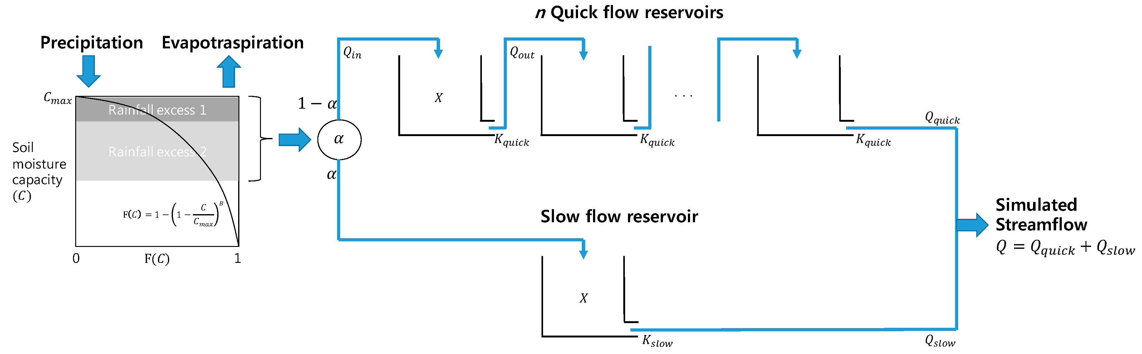
The original HYMOD model is a conceptual lumped RR model based on the probability-distributed principle [67]. The model consists of a simple two-parameter rainfall excess model linked with two series of parallel linear reservoirs for flow routing: three quick flow tanks and a slow flow tank. The distribution between the quick and slow flow tanks is adjusted by the parameter α, where 1-α is used for quick flow, and α is used for slow flow. Figure 3 shows a schematic diagram of the model structure.

The model assumes that a basin consists of soil moisture storage with varying capacity. The spatial variability of soil moisture capacity (C) is represented by the following cumulative distribution function:

$$\mathrm{F}(C)=1-{(1-\frac{C}{C_{\max }})}^B,$$

(11)

where C_max is the maximum storage capacity of the basin, and B is the degree of spatial variability of the soil moisture capacity of the basin. The time-varying total water storage of the basin (S(t) $\le \frac{C_{\max }}{B+1}$) is simulated by assuming that all storage within the basin is filled to the same critical level. Surface runoff is generated from a saturated area, whereas water is infiltrated into unsaturated areas. Further details on the rainfall excess model have been reported by Moore [67,68]. Therefore, the two parameters in the distribution function of soil moisture capacity, C_max and B, are important parameters to be calibrated.

The outflow from a reservoir (Q_out(t) in mm/day) and the reservoir state (X(t) in mm) during the time interval t are calculated following the assumption of a linear reservoir and mass conservation, respectively, as

$$Q_{out}(t)=K\times X(t)$$

(12)

$$X(t+\Delta t)=X(t)-(Q_{out}(t)+Q_{in}(t))\Delta t,$$

(13)

where K is the leakage rate in 1/day, which is identical to K_quick from the quick flow tanks and K_slow from the slow flow tank, and Q_in(t) is the inflow into the reservoir at time interval t. Inflow to a reservoir on the quick flow pathway can be either outflow from the basin or Q_out from another tank.

This study used a modified HYMOD model, which considers the number of quick flow reservoirs (n) as a parameter to be calibrated. Therefore, the timing of quick flow release to the river channel or the residence time of the quick flow reservoirs can be determined for a specific watershed.

Table 2. Summary of the six parameters in the modified hydrological model (HYMOD) used in this study.

Parameter	Definition (Units)	Lower Bound	Upper Bound
Cmax	Maximum storage capacity (mm)	50	600
B	Shape parameter of the probability distribution of the soil moisture capacity	0.05	1.95
α	Ratio of the distribution of the flow between quick and slow reservoirs	0.01	1
n	Number of quick flow reservoirs	1	4
Kslow	Conductivity of slow flow reservoir (1/day)	0.001	0.1
Kquick	Conductivity of quick flow reservoir (1/day)	0.1	0.95

summarizes the definition and range of the six parameters to be calibrated.

3. Case Study

A benchmark hydrological calibration test case for the Leaf River (1950 km²) near Collins, Mississippi, was used to examine the proposed balancing approaches. The Leaf River case study has been widely used for single and multiobjective hydrological model calibrations [8,9,12,27,53,69,70]. The two inputs are daily precipitation (mm/day) and potential evapotranspiration (mm/day; Figure 3). Daily streamflow (mm/day) and the two inputs were obtained from the National Weather Service Hydrology Laboratory. Initial storage in the watershed (i.e., initial basin storage and initial storage for quick and slow flow reservoirs) is assumed to equal zero, which indicates that they are empty. In order to remove the influence of the initial state, the HYMOD model was run for 15 days in a warm-up period. Here, a year of historical hydrological data, from 1 October 1948, to 30 September 1949, was used for model calibration, with annual mean streamflow of 2.62 mm/day (Figure 4b). The mean and standard deviations of the performance metrics were obtained for each of the static and variable approaches from 10 independent trial runs to consider the variability of the optimization results. Each optimization began with randomly generated model parameters with bounds as listed in Table 2. Further details of the Leaf River calibration problem and data can be found in previous studies [8,70,71,72,73].

4. Application Results

Figure 5 shows the procedures followed to compare the static and variable balancing approaches for the multiobjective calibration of the HYMOD model. First, two objectives considered in the multiobjective optimization are determined. Second, NPOP and NGEN suitable for the HYMOD model and the multiobjective calibration are selected. Then, several static approaches are compared to identify the best static approach. Finally, the static and variable approaches are compared to find the best approach. The following subsections describe the result of each step in Figure 5.

4.1. Numerical Experiment Setup

To select the two objectives, a scatter plot of a pair of the MAIs summarized in Table 1 was drawn for visual inspection for detecting the potential correlation between two indicators using a fitted linear regression line. Figure 6 shows the scatter plot of representative pairs: NSF versus Total MSE (TMSE) (Figure 6a), TMSE versus TPFD (Figure 6b), PB versus TPFD (Figure 6c), and NSF versus PB (Figure 6d). Although a perfect linearly negative correlation exists between NSF versus TMSE such that increasing the TMSE will result in decreasing the NSF (Figure 6a), a moderate linearly positive correlation exists between TMSE and TPFD (Figure 6b). Although the points were scattered widely around the fitted linear regression line, a trade-off relationship is expected to exist between PB and TPFD (Figure 6c). It appears that finding non-dominating points will provide valuable information for the optimal relationship between the two indicators (e.g., marginal TPFD changes with respect to the unit increase of PB). The Pearson correlation coefficient of representative pairs among TPFD, NSF, PB, and TMSE is summarized in

Table 3. Correlation coefficient of representative pairs of model accuracy indicators (MAIs) in Table 1.

	TPFD	NSF	PB	TMSE
TPFD	1.0
NSF	−0.455	1.0
PB	−0.228	−0.049	1.0
TMSE	0.504	−1.0	0.086	1.0

Notes: TPFD: Three Peak Flow Difference; NSF: Nash–Sutcliffe Measure; PB: Percent Bias; TMSE: Total Mean Squared Error.

. It should be noted that although the negative coefficient value was close to zero (Table 3), a no trade-off relationship might exist between NSF and PB, which is shown as a potential linear relationship at the right lower corner of the scatter plot (Figure 6d).

Therefore, minimizing TPFD and minimizing PB were selected as the two objectives of Equation (1) (i.e., f₁ = PB and f₂ = TPFD). The three largest peak flows occurred during the study year on 1 December 1948; 1 April 1949; and 2 May 1949, on Days 61, 183, and 214, respectively (Figure 5b). The absolute error between the observed and simulated streamflow for the three times was used for calculating TPFD (Table 1).

In this study, the four proposed variable balancing approaches for the exploration and exploitation of NSGA-II with SBX and PM were compared to the static balancing approaches using the performance metrics, SQM, SPM, and COM. In the static approaches, where C_DI and M_DI are kept constant during optimization (Figure 2), three sets of the parameters are applied following Zhang et al. [28]: (C_DI, M_DI) = (0.5, 0.5), (2.0, 0.5), and (20, 20). In total, seven balancing approaches were compared using three different Crates, Crate = 0.9, 0.75, and 0.6, which controls the frequency of visiting SBX and PM. Note that this study assumed that Crate was kept constant during optimization following Zhang et al. [28].

Table 4. Parameter values of the experiments.

Crossover and Mutation Rates (Crate)	Static Balancing Approaches (Three Cases) (CDI, MDI)	Variable Balancing Approaches (Four Cases)
0.6	(0.5, 0.5)	PSF1 for CDI and MDI
0.75	(2.0, 0.5)	PSF2 for CDI and MDI
0.9	(20, 20)	PSF1 for CDI and PSF2 for MDI
		PSF2 for CDI and PSF1 for MDI

Notes: C_DI: crossover distribution index; M_DI: mutation distribution index; PSF1: parameter-setting-free method that increases the algorithm parameter value from its minimum to maximum; PSF2: PSF that decreases the algorithm parameter value from its maximum to its minimum.

summarizes the parameter values and the method of the experiments considered.

4.2. Selection of the Appropriate Number of Populatiosn and Generations

First, this study performed a sensitivity analysis of the NPOP and NGEN on the performance of NSGA-II with SBX and PM. Before comparing the aforementioned balancing approaches, the appropriate NPOP and NGEN should first be identified as suitable for the complexity of the modified HYMOD model with six parameters. The combinations of NPOP of 30, 50, and 100 and NGEN of 100, 500, and 1000 (nine cases) were applied to the multiobjective model calibration and were compared with respect to SQM, SPM, and COM. Ten independent runs with randomly generated initial populations were performed to guarantee the reliability of the results. A Crate of 0.9 was used [28] with the constant C_DI and M_DI of (20, 20). To quantify the three performance metrics, the global Pareto solutions Z* were first identified by gathering and non-dominatedly sorting all Pareto solutions found from the nine cases.

Figure 7 shows 511 global Pareto solutions (Z*) identified from the non-dominated sorting of 5400 (=10 independent runs × 3 NGEN cases × (30 + 50 + 100)) Pareto solutions obtained from the optimization of the nine cases (i.e., 9.46% of the Pareto solutions were the global Pareto solutions). No point was located at the lower-left corner of the global Pareto solutions because no solutions were found with a lower PB and lower TPFD than those solutions (Figure 7).

Several statistics of SQM (i.e., total SQM, mean SQM, and standard deviation (stdv) of SQM) and the mean value of SPM and COM are summarized in

Table 5. Performance metrics of combinations of the nine cases of the number of populations (NPOP) and the number of generations (NGEN). The total number of global Pareto solutions is 511.

		NPOP = 30	NPOP = 50	NPOP = 100
NGEN = 100	Total SQM	1	3	60
	Mean SQM (stdv)	0.1 (0.316)	0.3 (0.675)	6 (5.907)
	Mean SPM	0.798	0.621	0.994
	Mean COM	0.127	0.057	0.061
NGEN = 500	Total SQM	24	40	232
	Mean SQM (stdv)	2.4 (2.989)	4 (5.033)	23.2 (6.647)
	Mean SPM	0.703	0.820	0.825
	Mean COM	0.026	0.048	0.014
NGEN = 1000	Total SQM	1	28	122
	Mean SQM (stdv)	0.1 (0.316)	2.8 (1.814)	12.2 (4.872)
	Mean SPM	0.826	0.855	0.895
	Mean COM	0.058	0.031	0.066

Notes: SQM: solution quality metric; SPM: spacing metric; COM: convergence metric; stdv: standard deviation.

. The total SQM is the total number of global Pareto solutions found from 10 independent optimization runs for a case. The mean SQM is an expected value of SQM for a single optimization run, calculated as the total SQM divided by 10. The stdv of the SQM is a robustness measure that indicates the variation of the algorithm performance over the runs. Therefore, greater values of total SQM and mean SQM are preferred, whereas smaller values are favorable for the stdv of SQM.

Although an NPOP of 30 resulted in the poorest performance (e.g., total SQM = 1 for the cases NGEN = 100 and 1000), NPOP = 100 guaranteed the best performance with respect to SQM. NPOP had a greater impact on the algorithm performance than NGEN. In this study, NPOP = 100 and NGEN = 500 were selected for testing the static and variable balancing approaches because they yielded the greatest number of global Pareto solutions, where 45.4% of the global Pareto solutions were identified by this case, and the smallest mean COM value of 0.014 (gray filled cases in Table 5). The mean COM of the second-best case, NPOP = 100 and NGEN = 1000, was 0.066 (Table 5). It should be noted that the coefficient of variation of the SQMs of the selected case (CV = 6.647/23.2 = 0.287) was lower than the second-best case (CV = 4.872/12.2 = 0.399), indicating the production of more reliable final solutions.

4.3. Comparison of the Static and Variable Balancing Approaches

This study compared the static and variable balancing approaches in three steps. First, the static approaches with nine different Crates, C_DI, and M_DI sets were compared to identify the best static balancing approach. Ten independent runs were performed by using each combination of the nine cases (Table 4). Then, all Pareto solutions were gathered to identify the global Pareto solutions. A total of 990 global Pareto solutions was obtained, which was 11% of all Pareto solutions from the nine cases. The SQM, SPM, and COM were calculated using the identified global Pareto solutions and are summarized in

Table 6. Performance metrics of the nine cases of the crossover rate (Crate) and (crossover distribution index (C_DI) and mutation distribution index (M_DI)) combinations. The total number of global Pareto solutions is 990.

		(CDI, MDI)
		(0.5, 0.5)	(2.0, 0.5)	(20, 20)
Crate = 0.6	Mean SQM (stdv)	10.6 (3.8)	12.5 (5.8)	13.9 (15.8)
	Mean SPM	0.828	0.761	0.850
	Mean COM	0.008	0.006	0.088
Crate = 0.75	Mean SQM (stdv)	10.7 (5.0)	12 (5.8)	12.4 (14.7)
	Mean SPM	0.829	0.793	0.777
	Mean COM	0.008	0.007	0.008
Crate = 0.9	Mean SQM (stdv)	8.8 (2.9)	8.2 (3.7)	9.9 (4.0)
	Mean SPM	0.805	0.766	0.749
	Mean COM	0.012	0.012	0.009

Notes: SQM: solution quality metric; SPM: spacing metric; COM: convergence metric; stdv: standard deviation.

. The greatest number of global Pareto solutions was found from the case Crate = 0.6 and (C_DI, M_DI) of (20, 20). The case Crate = 0.6 and (C_DI, M_DI) of (2.0, 0.5), guaranteed the closest Pareto solutions to the global Pareto front, where the mean COM was 0.006. This result is different from the best parameter set found by Zhang et al. [28]. They confirmed that (C_DI, M_DI) of (0.5, 0.5) resulted in the best performance among the three sets of (C_DI and M_DI) with a Crate of 0.9 in a multiobjective parameter calibration of a SHETRAN model minimizing the RMSE and minimizing the LOGE. Therefore, we confirmed that the best algorithm parameter set varies depending on the complexity of the hydrological model and the formulation (e.g., the considered objective function) of the optimal calibration model.

Second, the best variable balancing method was identified among the 12 cases, which included combinations of Crates of 0.6, 0.75, and 0.9 and Approaches 1 to 4 (Table 4). The Crate was fixed during optimization, whereas C_DI and M_DI varied over generations using either PSF1 or PSF2. A total of 805 global Pareto solutions was identified, which is 6.7% of all Pareto solutions from the 12 cases. The solutions were compared with those found from the first step (i.e., static balancing cases).

Figure 8a shows all of the Pareto fronts obtained from the two balancing approaches; their global Pareto fronts are drawn in Figure 8b. It was confirmed that the global Pareto solution of the variable approaches dominated that of the static approaches, indicating that the former outperformed the latter. The gap between the two global fronts was significant as the inferiority level of the latter. Using fixed C_DI and M_DI (i.e., static approach) would result in providing false information regarding the trade-off relationship between the two objectives to decision makers (Figure 7 and Figure 8b). For example, the global Pareto solution of the TPFD of 6 mm/day resulted in a PB of 4.7% in the variable approach and 13.1% in the static approach.

Finally, the global Pareto front was extracted from all Pareto solutions of all static and variable cases to quantify the performance metrics and to confirm the results from the second step.

Table 7. Performance metrics of all 21 static and variable cases. The total number of global Pareto solutions is 805.

		Static Approach (CDI, MDI)			Variable Approach (Table 4)
		(0.5, 0.5)	(2.0, 0.5)	(20, 20)	Approach 1	Approach 2	Approach 3	Approach 4
Crate = 0.6	Mean SQM (stdv)	0	0	0	0	0	22.3 (4.138)	16.9 (5.705)
	Mean SPM	2.081	1.525	1.241	1.278	1.597	1.269	1.299
	Mean COM	0.189	0.175	0.255	0.193	0.228	0.017	0.013
Crate = 0.75	Mean SQM (stdv)	0	0	0	0	0	0.1 (0.316)	0
	Mean SPM	2.081	2.023	1.945	1.266	1.180	1.280	1.599
	Mean COM	0.186	0.201	0.181	0.158	0.232	0.191	0.194
Crate = 0.9	Mean SQM (stdv)	0	0	0	0	0	19.9 (7.880)	21.3 (4.084)
	Mean SPM	1.801	1.646	1.416	1.426	1.551	1.138	1.149
	Mean COM	0.214	0.208	0.194	0.206	0.218	0.062	0.011

Notes: C_DI: crossover distribution index; M_DI: mutation distribution index; Crate: crossover rate; SQM: solution quality metric; SPM: spacing metric; COM: convergence metric; stdv: standard deviation. Mean SQM is 4.3 when it is assumed that all methods are performed equally. Note that a case with a mean SQM of zero indicates no global Pareto solution was found. The metrics SPM and COM are relative measures. For example, a method with a mean SPM of 2.081 produces a Pareto front 168% wider than that of an approach with a mean SPM of 1.241. Similarly, a method with a mean COM of 0.255 indicates a Pareto front 1962% farther from the global Pareto front compared to an approach with a mean COM of 0.013.

summarizes the valued of SQM, SPM, and COM of the 21 total cases (=9 static cases + 12 variable cases). As expected, the mean SQMs of the static approach is zero, indicating the Pareto solutions obtained by the static approach are inferior to those obtained by the variable approach. The mean SPM and COM values of the variable approaches were significantly lower than those of the static approaches, which indicates that the former produced a more converged solution with a widespread front.

Most global Pareto solutions were identified by Approaches 3 and 4 when using Crates of 0.6 and 0.9 (gray filled cases in Table 7). Approaches 3 and 4 changed the focus of the exploration and exploitation differently for SBX and PM. For example, Approach 3 focused on the exploration (C_DI begins at 0.5) in the early phase and the exploitation (C_DI approaches 20) in the latter phase for SBX and considers the opposite for PM (Figure 1 and Figure 2). Considering the same exploration and exploitation variations (Approaches 1 and 2) resulted in poor performance (Table 7).

For a high Crate (i.e., 0.9), Approach 4 outperformed Approach 3 with respect to all three performance metrics (Table 7). For a low Crate of 0.6, Approach 3 performed better than Approach 4 with respect to SQM, whereas SPM and COM were similar. The global Pareto solutions found by Approach 3 with a Crate of 0.6 and those by Approach 4 with a Crate of 0.9 were located throughout the entire front (Figure 8c), indicating the ability to develop widespread Pareto solutions. Interestingly, an intermittent level of crossover rate (i.e., Crate of 0.75) resulted in poor performance compared with the other variable approach cases. Therefore, a careful sensitivity analysis should also be conducted on the fixed Crate to be used with variable approaches.

4.4. Calibrated Parameters and Hydrographs

The solutions were positioned on different parts of the Pareto front. To determine the cause of this result, the calibrated values of the six parameters of the HYMOD model (Table 2) were inspected. Figure 9 shows the parameter ranges of the global Pareto solutions obtained by the variable balancing approaches, and the Pareto front is shown in Figure 8 and Figure 10. It should be noted that the plotted values in Figure 9 are the normalized parameter values using each parameter’s maximum value (Table 2). It was found that the final parameter sets can be classified into two groups: one with two quick flow reservoirs (Group 1) and the other with a single quick flow reservoir (Group 2). Each group had distinctively different ranges for some parameters (Figure 9). For example, Group 1 had a shape parameter B of less than 0.026 and quick and slow flow distribution ratios α of about 0.6 (Figure 9). In addition, the leakage rate of the slow flow reservoir K_slow was close to 0.1/day for all solutions in Group 1. In contrast, Group 2 had B values between 0.1 and 0.42 and α close to 1. K_slow had a wide range of values.

Because of such differences in the parameter values, the solutions with two quick flow reservoirs were located in the low PB and high TPFD region of the global Pareto front, whereas those with a single quick flow reservoir were located in the medium-to-high PB and low TPFD regions (Figure 10).

Most rainfall excess is directed to slow flow tanks when α is close to 1 (Figure 3). Therefore, the contribution of a single quick flow reservoir is negligible to the final discharge of the HYMOD model in Group 2 (n = 1 and α close to 1). In addition, its K_quick value was lower than that for Group 1 (n = 2) (Figure 3 and Figure 8). Conversely, the parameter values of Group 1 (n = 2) were in the physically sound ranges in which about 40% of the rainfall excess flowed to a series of two quick flow tanks with K_quick of approximately 0.54/day and a single slow flow tank with K_slow close to 0.1/day (Figure 9).

Finally, the three simulated hydrographs were compared with the observed hydrograph (Figure 11). The two simulated hydrographs were obtained by using: (1) the lowest PB (PB of 3.04 × 10⁻⁸ and TPFD of 9.07 mm/day; simulated hydrograph 1); and (2) the lowest TPFD (PB of 29.71% and TPFD of 3.96 mm/day; simulated hydrograph 2). These two solutions are located at each end of the global Pareto front (Figure 10), representing a hydrograph obtained by using parameters of Group 1 and Group 2, respectively. A simulated hydrograph of PB of 1.87% and TPFD of 8.35 mm/day was also plotted (simulated hydrograph 3) as a reference hydrograph. The three peak flow observations are labeled Peak 1, Peak 2, and Peak 3 in Figure 11.

It appears that simulated hydrograph 1, having the greatest TPFD, better fits the three peaks than the simulated hydrograph 2, having the lowest TPFD (Figure 11). However, Figure 12 shows that hydrograph 1 significantly sacrificed accurate prediction of the third peak flow (Peak 3) for the optimization of PB (Figure 12c). Because PB measures the difference between the means of the observed and simulated streamflows, more focus is put on adjusting the very high flows to match the two mean values. It should be noted that the flow magnitude observation of Peaks 1 and 2 are 56% and 71% greater than that of Peak 3, respectively. For this reason, the error for the day at Peak 3 of simulated hydrograph 1 was 8.39 mm/day (Figure 12c), whereas negligible error was present for the days for Peaks 1 and 2 (Figure 12a,b, respectively).

In contrast, simulated streamflow 2, having the lowest TPFD, was well matched to the observed streamflow on all three peak days (Figure 12a–c). However, greedy blind searching characteristics of the automatic calibration were detected. That is, in order to minimize the TPFD, the streamflow value at a time interval before the peak day was increased or the concentration time of peak flow was shortened, resulting in moderate to high error on the first two peak days (Peaks 1 and 2; Figure 11a,b). Because matching the simulated streamflow only at the three time intervals, at days 183 (Figure 12a), 61 (Figure 12b), and 214 (Figure 12c), is the objective considered in the multiobjective calibration model (Equation (1)), errors in the neighborhood time intervals were not considered. Therefore, it is recommended that the sum of the absolute error at the peak flow days and the error at their neighborhood time intervals at both sides of the rising and falling limbs be considered when formulating peak flow accuracy measures. A hydrologist should pay very careful attention in selecting and formulating objective functions when employing automatic parameter calibration of a hydrological model.

5. Discussion

This study has several limitations that should be addressed by future research. First, the proposed balancing approaches should be compared with the traditional static approaches in the single and multiobjective calibration of hydrological models with different levels of complexity (e.g., a spatially distributed hydrological model). In addition, such comparison can be conducted in a multiobjective parameter calibration with different sets of competing objectives and more than two objectives. From thorough investigations, a generalized conclusion on how to improve solution quality and guarantee the best performance can be derived to serve as a guideline for automatic parameter calibration of hydrological models. Second, this study assumed a Crate of NSGA-II as a fixed value. However, the Crate can be varied over generations, as with C_DI and M_DI, such that the best performing method could be different from our findings. The final Pareto solutions were used for the comparison of different balancing approaches in this study. However, run-time searching behavior of the approaches could also be investigated by employing run-time performance metrics (e.g., Zheng et al. [45]).

6. Summary and Conclusions

This study proposed variable balancing approaches for the exploration and exploitation of NSGA-II with SBX and PM in the multiobjective automatic parameter calibration of a lumped hydrological model, the HYMOD model. Six model parameters for maximum storage capacity, soil moisture capacity distribution, ratio between quick and slow flows, the number of quick flow reservoirs, and leakage rates for quick and slow flow tanks were used. The two objectives of minimizing the percent bias and minimizing the sum of the absolute error at three peak flow days were selected by visual inspection, linear regression, and Pearson correlation analysis of a pair of various MAIs quantified by using randomly generated model parameter values. The proposed balancing approaches, which migrate the focus between exploration and exploitation over generations by varying C_DI and M_DI, were compared with traditional static balancing approaches (the two dices value is fixed during optimization) in a benchmark hydrological calibration problem for the Leaf River (1950 km²) near Collins, Mississippi. Three performance metrics, the solution quality, spacing, and convergence (SQM, SPM, and COM, respectively), were used to quantitatively compare the performance of the two different balancing approaches. NPOP = 100 and NGEN = 500 were selected from sensitivity analysis and were used for optimization.

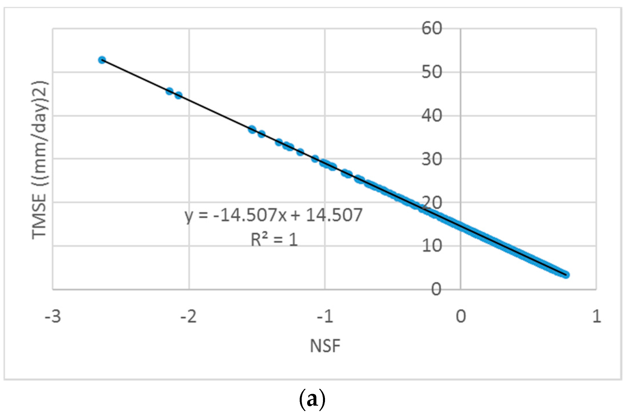
First, a scatter plot of a pair of the MAIs summarized was drawn for visual inspection for detecting the potential correlation between two indicators by using a fitted linear regression line. A trade-off relationship was found between PB and TPFD. PB measures the difference between the means of the observed and simulated streamflows, whereas TPFD calculates the sum of three peak flow differences. The Pearson correlation coefficient between the two measures was −0.228, indicating a negligible correlation exists.

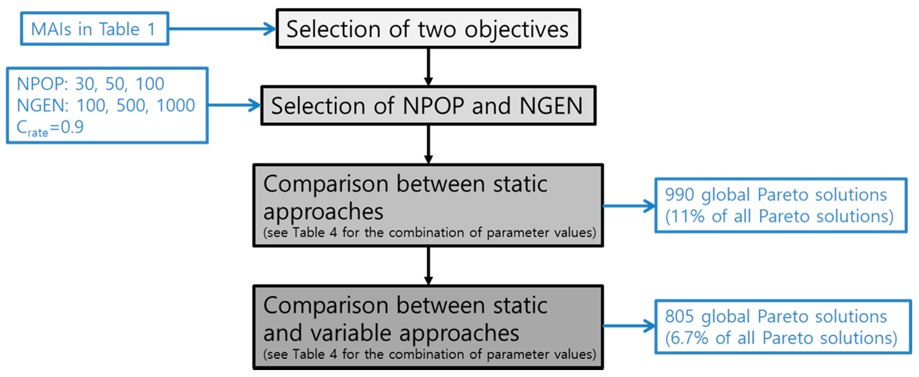
Then, the best static approach was identified from nine cases of Crate and (C_DI, M_DI) with combinations of Crates of 0.6, 0.75, and 0.9 and (C_DI, M_DI) values of (0.5, 0.5), (2.0, 0.5), and (20, 20). A high value of C_DI (or M_DI) results in children solutions that are more similar to the parent solutions (exploitation), whereas small values of C_DI (or M_DI) emphasize exploration. It was found that a Crate of 0.6 and (C_DI, M_DI) of (2.0, 0.5) and (20, 20) resulted in the best performance. The greatest number of global Pareto solutions (mean SQM = 13.9) was found in the case (C_DI, M_DI) of (20, 20), and the best convergence (mean COM = 0.006) was observed in the case (C_DI, M_DI) of (2.0, 0.5). These results are different from those of Zhang et al. [28], who found the best performance with a Crate of 0.9 and (C_DI, M_DI) of (0.5, 0.5) in the calibration of a spatially distributed hydrological model. Therefore, sensitivity analysis on the algorithm parameters should be conducted to identify the best parameter set, particularly when an algorithm for use has not been previously combined with a hydrologic model.

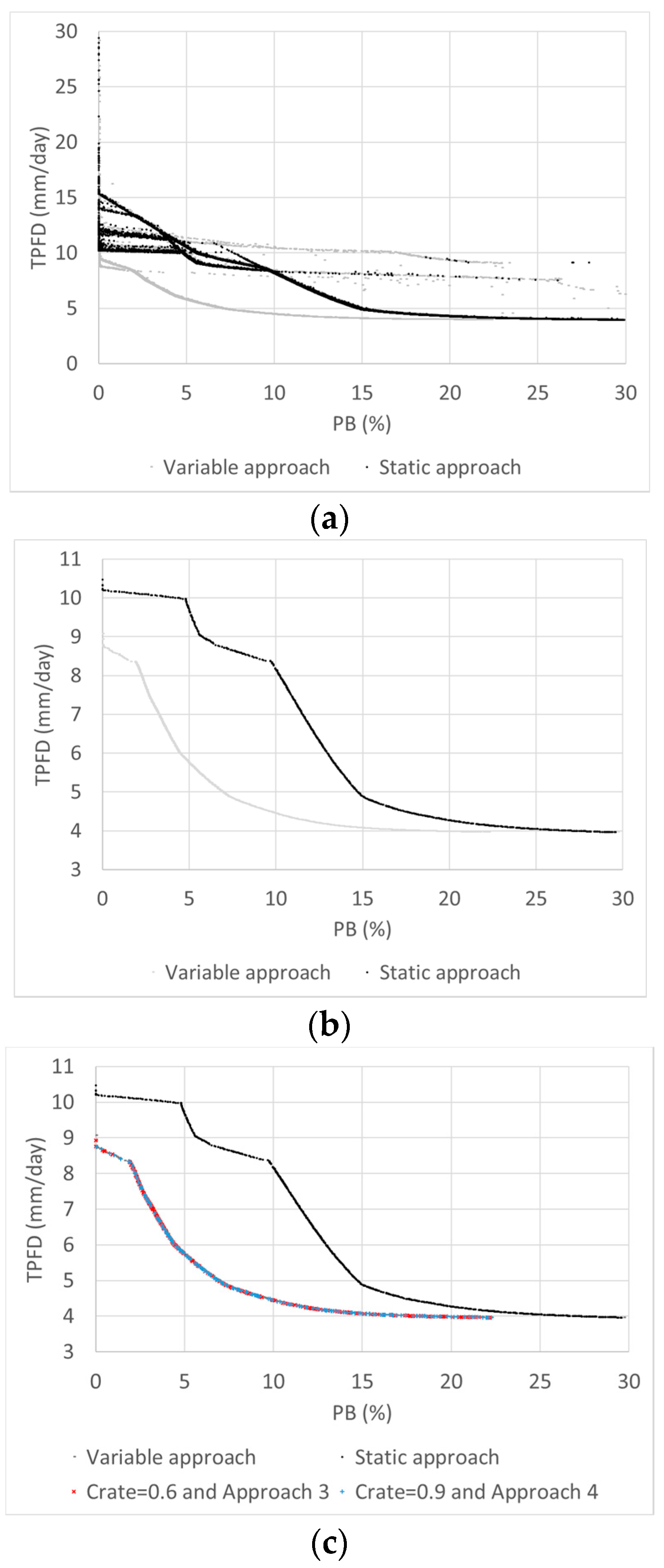
The overall best balancing approach was determined from the comparison of the nine static approaches and 12 variable approaches. Twelve cases of the variable approaches were generated from the combinations of Crate of 0.6, 0.75, and 0.9 (three cases) and four approaches for variable C_DI and M_DI (Approaches 1 to 4). Although the variable approaches with Crates of 0.6 and 0.9 and Approaches 3 and 4 outperformed other approaches, the greatest number of global Pareto solutions was found from the variable cases with a Crate of 0.6 and Approach 3 and with a Crate of 0.9 and Approach 4. Approaches 3 and 4 migrate the focus of exploration and exploitation differently for SBX and PM, which results in better performance than that with Approaches 1 and 2 using the same variable balancing scheme.

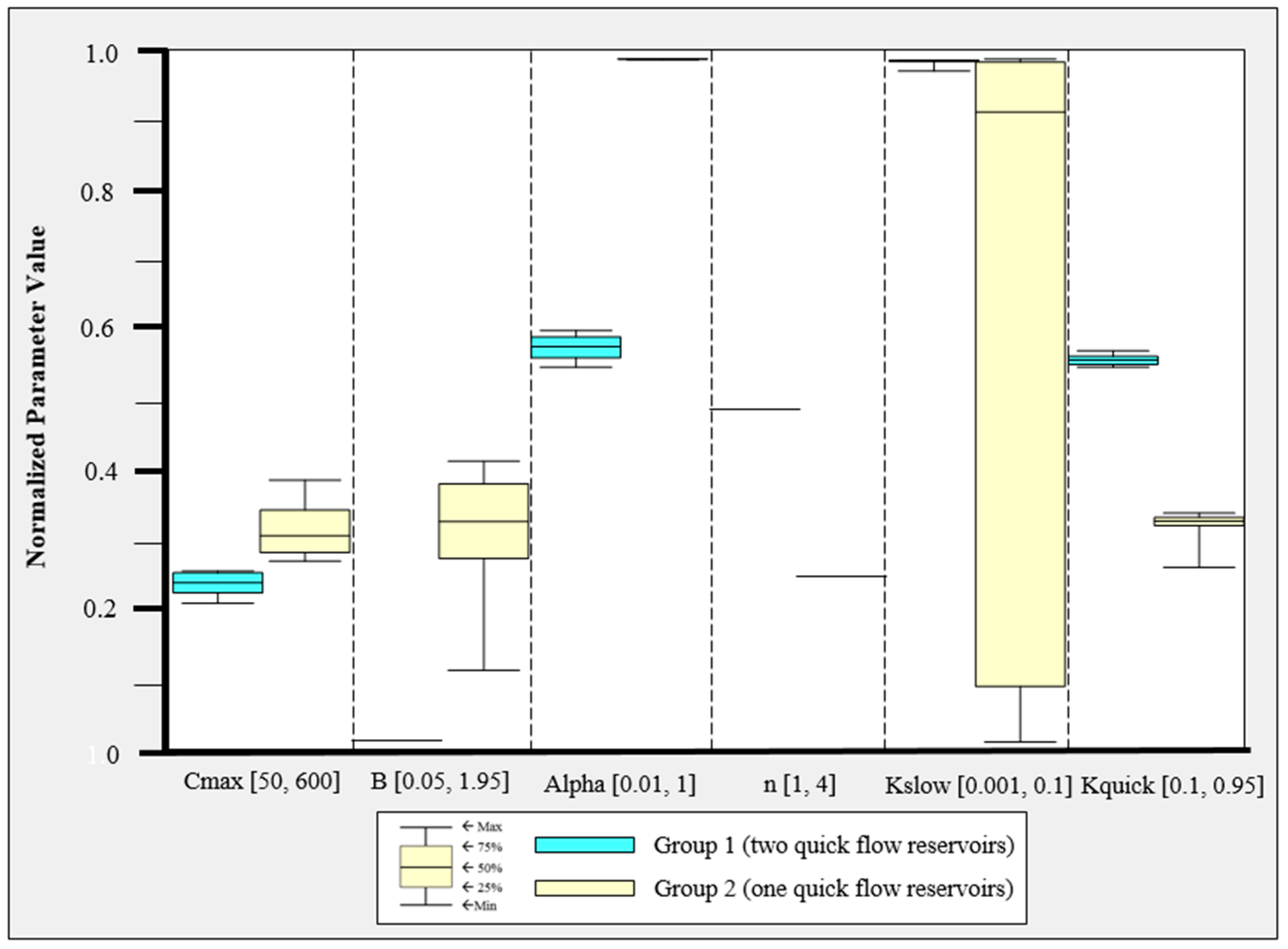
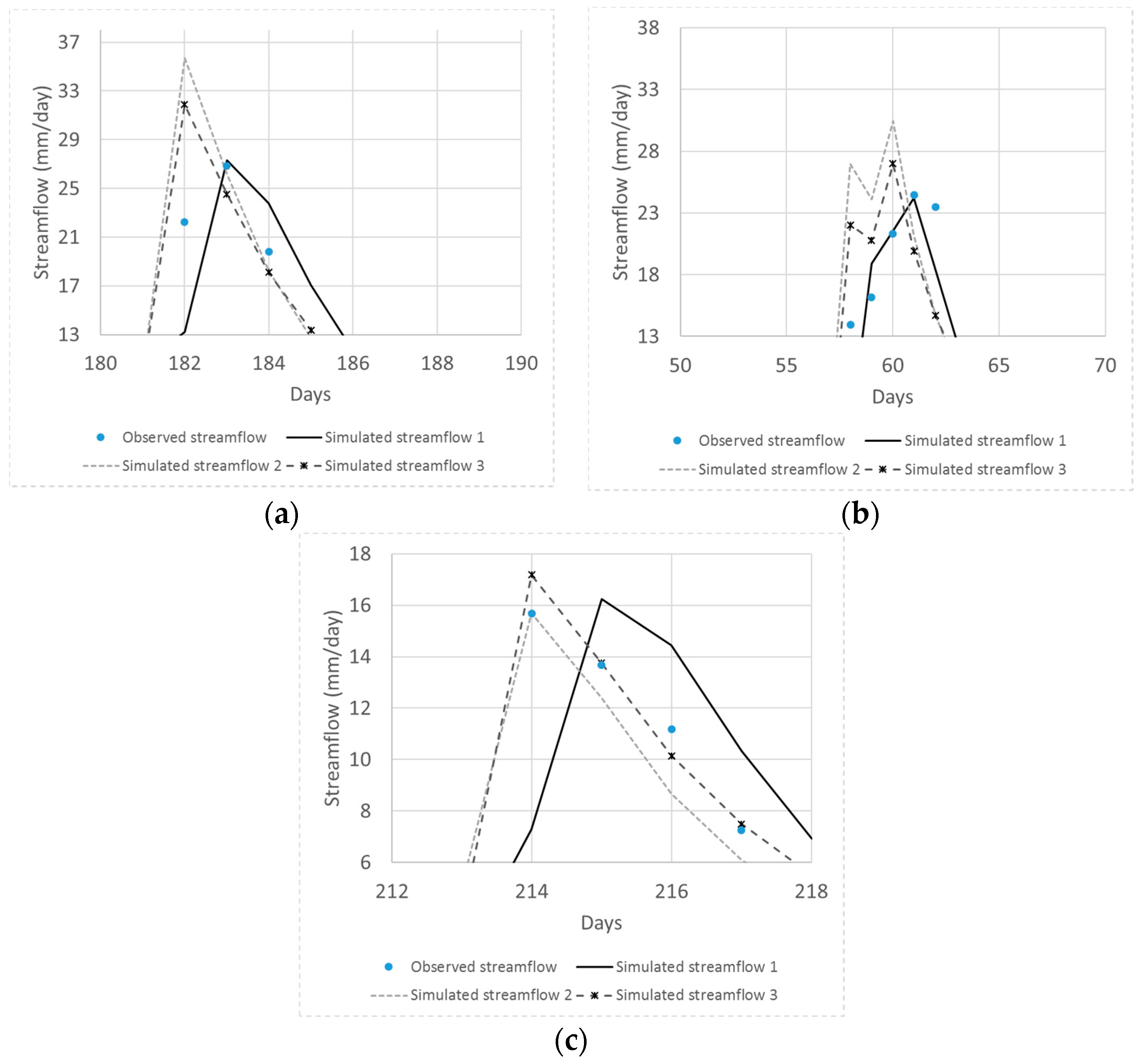
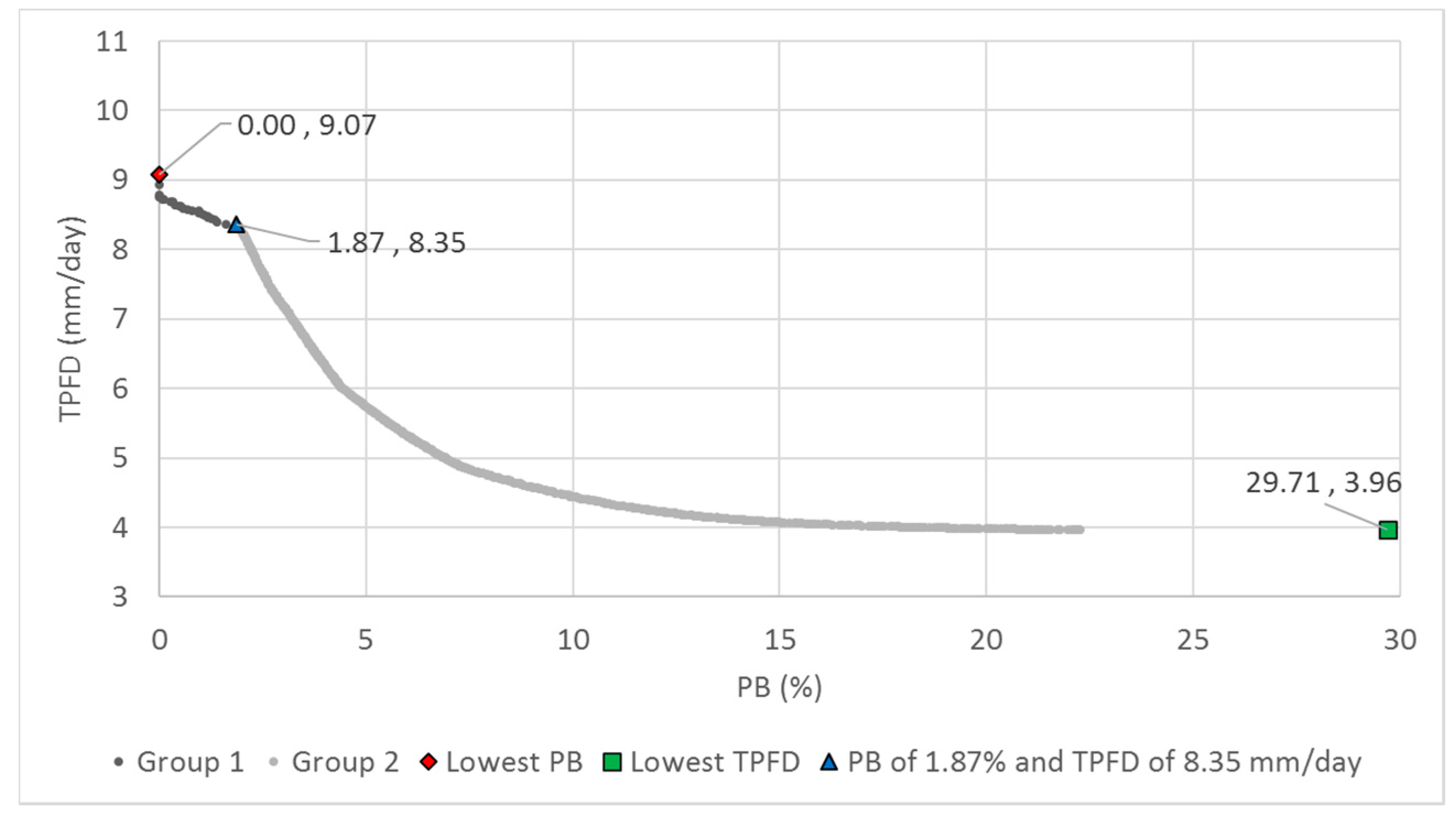
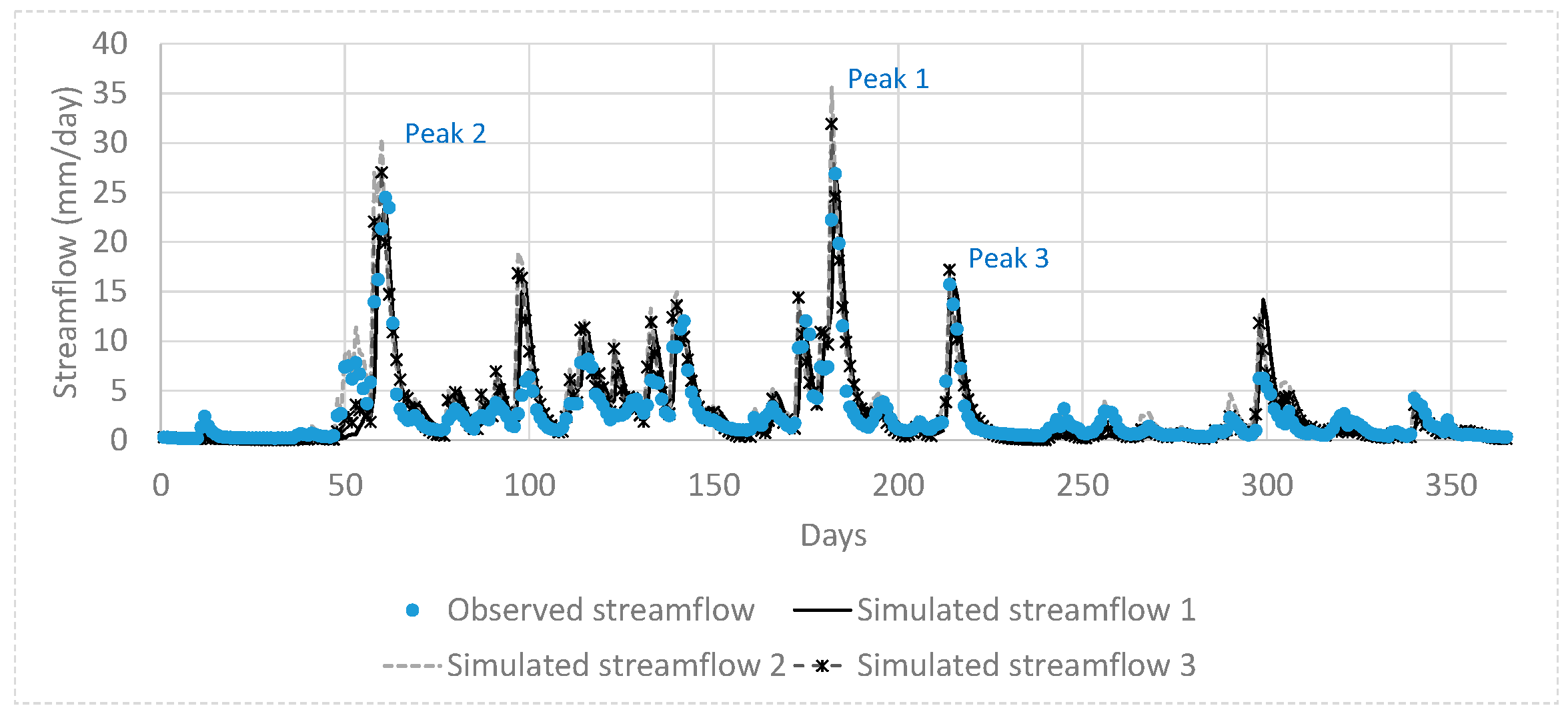
Finally, the parameter ranges of the global Pareto solutions were examined to determine which differences in model parameter values result in different objective function values. The global Pareto parameter set with two quick flow reservoirs resulted in low PB and high TPFD, whereas that with a single quick flow reservoir had irregular parameter values. In addition, three representative simulated hydrographs and the observed hydrograph were compared. Greedy blind searching characteristics of the automatic calibration were detected from the global Pareto solutions with a single quick flow reservoir. That is, the error at neighboring times of peak flow days was increased in order to minimize TPFD. The low PB solutions sacrificed the accuracy of the smallest of the three peak flows. It is recommended that the sum of the absolute error at the peak flow days and the error at their neighborhood time intervals at both sides of the rising and falling limbs be considered when formulating peak flow accuracy measures.