Abstract
A new methodology for estimating the discharge starting from the monitoring of surface flow velocity, usurf, is proposed. The approach, based on the entropy theory, involves the actual location of maximum flow velocity, umax, which may occur below the water surface (dip phenomena), affecting the shape of velocity profile. The method identifies the two-dimensional velocity distribution in the cross-sectional flow area, just sampling usurf and applying an iterative procedure to estimate both the dip and umax. Five gage sites, for which a large velocity dataset is available, are used as a case study. Results show that the method is accurate in simulating the depth-averaged velocities along the verticals and the mean flow velocity with an error, on average, lower than 12% and 6%, respectively. The comparison with the velocity index method for the estimation of the mean flow velocity using the measured usurf, demonstrates that the method proposed here is more accurate mainly for rivers with a lower aspect ratio where secondary currents are expected. Moreover, the dip assessment is found more representative of the actual location of maximum flow velocity with respect to the one estimated by a different entropy approach. In terms of discharge, the errors do not exceed 3% for high floods, showing the good potentiality of the method to be used for the monitoring of these events.
1. Introduction
The estimate of a reliable discharge is tightly connected to a robust velocity dataset where the mean flow velocity is inferred using velocity measurements carried out for high water levels. This condition is not so usual considering that at hydrometric sites the most common technique used for velocity sampling is based on the current meter from the cableway, and measuring velocity points during high floods in the lower portion of flow area is difficult and dangerous for operators [1]. The stage monitoring is straightforward and relatively inexpensive compared with the cost necessary to carry out flow velocity measurements, which are, however, limited to low flows and constrained by the accessibility of the site. Therefore, the discharge estimation is often obtained by extrapolating the relationship between stage and the discharge obtained for velocity measurements referring to low flows, and, as a consequence, a high uncertainty holds in the assessment [2]. For high flow, the mean flow velocity is hard to estimate, affecting de-facto the reliability of the discharge assessment for extreme events.
To date, ultrasonic devices, such as Acoustic Doppler Current Profilers (ADCP), can be adopted to address the velocity measure for high floods. Indeed, the introduction of ADCP on moving-vessels would allow operators to overcome the aforementioned issues, even if several limitations remain. During high floods, the magnitude of sediment transport may produce a reduction of the signal-noise ratio of acoustic sensors along with the capability of the signal to penetrate through the water [3]. In addition, high flow conditions, mean high velocity, and high turbulence can affect the water depth estimation because of the roll and pitch motions of the vessel [4] as well as vessel tracking [5]. The high velocity and high water levels represent big trouble for the operators considering that branches or trunks of trees can be carried by the flow and could still represent a risk for the instrument as well as the safety of the operators themselves.
On the other hand, the surface flow velocity can be easily monitored by using no-contact technologies as Surface Velocity Radar (SVR) [6,7] and/or Large Scale Particle Image Velocimetry (LSPIV) [8,9]. The radar technology may be affected during low flow when the backscatter of the beam can be blended by high noise, while LSPIV might be not suitable for measurements during scarce seeding, illumination conditions, and/or for any overnight floods [10]. However, the SVR and LSPIV, being no-contact techniques, are suitable for high flows monitoring, without encountering the issues connected to the floating surface material, sediment transport, and dangers for operators.
The information content given by SVR and LSPIV is the spatial distribution of surface flow velocity from which the discharge at a river site might be estimated. In this context, a focal point is how to turn the surface velocity, usurf, measured at a location (vertical) into depth-averaged velocity, uvert, considering the different hydraulic and geometric characteristics of river sites which affect the velocity profile shapes [11]. In the case of maximum flow velocity occurs on the water surface, the two-parameters power law velocity distribution developed by Dingman [12] could be applied to this end.
However, the aspect ratio W/D (with W the channel width and D the flow depth) unfolds a fundamental role on the characteristics of the velocity profile because the presence of the sidewalls may influence the velocity distribution, causing secondary currents that drive the maximum velocity below the water surface, so triggering the well-known dip phenomenon [13].
Overall, the surface velocities are transformed in depth-averaged velocity, assuming a monotonous velocity profile and multiplying the surface velocity, usurf, by a velocity index, k = uvert/usurf, equal to 0.85 (e.g., [7] for SVR and [9] for LSPIV). However, the possible occurrence of the dip phenomenon could make the assumption ‘weak’ for create flows where a monotonous velocity distribution does not take place. Consequently, the velocity index value might be not representative of the two-dimensional spatial velocity distribution anymore, leading to failure of the assessment of discharge.
The entropic velocity distribution developed by [14] can be used to cope with this matter. This approach established a bridge between the probability domain, wherein a probability distribution of the velocity is surmised, and the physical space by deriving the cumulative probability distribution function in terms of curvilinear coordinates in the physical space [15,16]. Therefore, it would be possible to relate the surface velocity measured by SVR and/or LSPIV across the river site, and the maximum velocity occurring below the water surface corresponding to the vertical where the surface velocity is sampled, as shown by [17]. In this context, the identification of the dip, i.e., the location where umax occurs below the water surface, is the main issue. The dip may significantly affect the estimation of the depth-averaged velocity from which, through the velocity area method, the mean flow can be assessed and, hence, the discharge.
This work is aimed to present a new methodology based on the entropy theory of estimating the discharge, starting from the surface flow velocity and taking the dip of the velocity profile into account. Moreover, remarks on the robustness of the velocity index using field data are discussed. The entropy method can be applied regardless of the technique adopted for the surface velocity measurement.
Five gage sites with different geometric and hydraulic characteristics are used as a case study.
The paper is organized as follows. Section 2 provides the theoretical background of the entropy method applied to measured surface flow velocities. Section 3 describes the case study along with the velocity dataset. Section 4 describes the results achieved for the five selected river gage sites and makes a comparison with the velocity index method. Finally, the last section features the conclusions drawn from this investigation.
2. Method
The method is based on the entropy probability density function of velocity, u, such as derived by [18] and simplified by [19] assuming that the entropy velocity profile at the y-axis, where the maximum flow velocity, umax, occurs, holds for all verticals in flow area, yielding:
where umaxv(xi) is the maximum velocity along the ith vertical, xi is the position of the ith sampled vertical from the left bank, M is the entropic parameter, h(xi) is the dip, i.e., the depth of umaxv(xi) below the water surface, D(xi) the vertical depth, y is the distance of the velocity point from the bed, and Nv is the number of verticals sampled across the river section. The entropic parameter M, which is a characteristic of the section [20], can be easily estimated through the pairs (um, umax) of the available velocity dataset at a gauge site by using the linear entropic relation [14]:
where um is the mean flow velocity and umax is the maximum flow velocity in flow area.
In addition, Moramarco [21] showed that, at a gauged river site, Φ(M) is constant for any flow conditions and its estimation can be addressed for ungauged sites as well by leveraging the dependence of Φ(M) on hydraulic and geometric characteristics.
Even if umaxv occurs below the water surface, it could be estimated for each vertical as a function of surface velocity, , such as proposed by [22]:
where . Specifically, if , it follows that and, hence, that . An application of Equation (3) in natural channels was done by [17], who calibrated a hydraulic model by leveraging the surface velocity measurements by SVR at different times.
2.1. Dip Estimate
Considering that the dip, is generally unknown across the flow area, a method is proposed here for its estimation. The approach exploits the experimental outcomes obtained by [13] who investigated the mechanism of the dip phenomenon by leveraging a laboratory channel velocity dataset. Specifically, it was found that for different aspect ratios W/D (with W the channel width and D the flow depth), the location of below the water surface, is mainly linked to the lateral position of the velocity profiles from the sidewalls. Based on this analysis, the dip phenomenon was more significant close to the banks and for large aspect ratio values, in accordance with the following relationship [13]:
It is worth noting that Equation (4) well represented the measured data obtained in different works dealing with smooth and rough natural channels and we refer to [13] for more details.
Placing Equation (4) into Equation (3) and both into Equation (1), the two-dimensional velocity distribution can be identified by leveraging the surface velocity measured by SVR or LSPIV. In this way, um and umax can be estimated using the velocity-area method [23], and, hence, can be computed by Equation (2) [19]. However, the uncertainty due to the presence of secondary currents lead us to modify Equation (4) in:
where is a parameter representing the dip at the y-axis and which is updated through an iterative process, wherein at each iteration, p, a constant value (0.1 m) is added to the initial value assumed to be equal to The iterative parameter refinement process ends by minimizing the objective function when the optimal value of is achieved in accordance with:
where is the threshold error, assumed equal to 0.01.
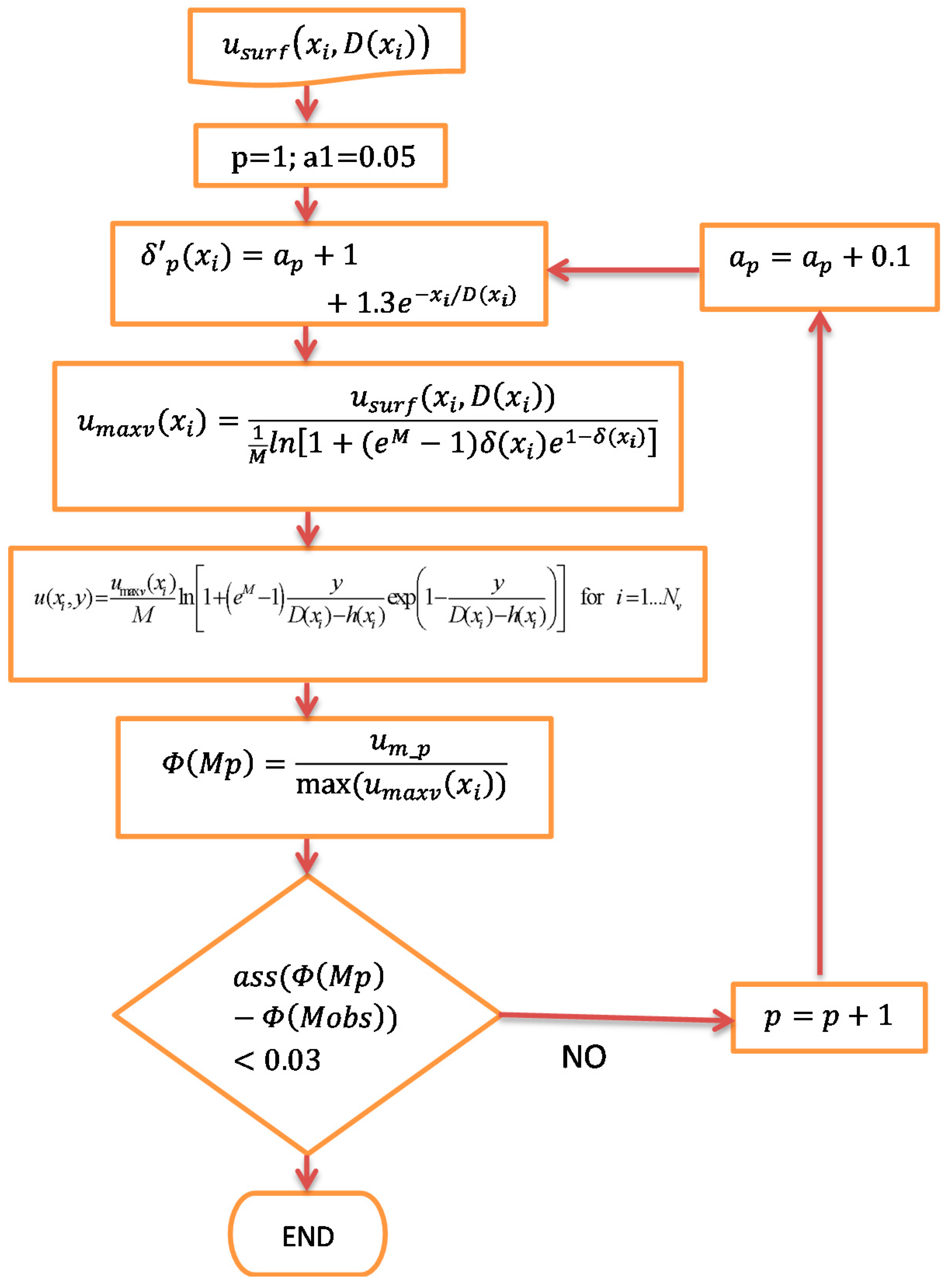
Steps of the procedure described above are detailed in the schematic diagram as shown in Figure 1. The method can be applied for gage sites in which a robust velocity dataset is available and Φ(Mobs) can be easily estimated by the observed pairs (um, umax). For ungauged sites, the M parameter can be even estimated by expressing its value in terms of hydraulic and geometric characteristics such as proposed by [21] and/or following [20], who identified a simple way to estimate M from the maximum surface velocity typically located near the middle of the channel [24].
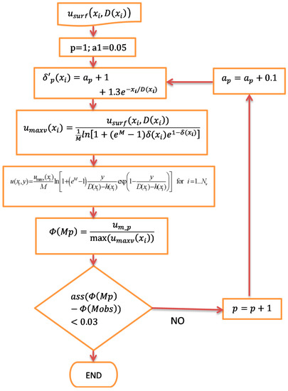
Figure 1.
Schematic representation of dip estimation procedure using measured surface velocity, usurf (for symbols see text).
For representing the dip in flow area, the relationship proposed by [25] may be also adopted:
Unlike the proposed method, Equation (7) does not need to consider an iterative procedure to estimate the dip along sampled verticals and would be simpler to apply. Specifically, Equation (7) provides h(xi) that can be used to estimate This implies the interest in comparing the two approaches. However, it is worth noting that our target is not to estimate the effectiveness of these relationships in the dip assessment but rather to analyze whether, if given a distribution of dip in flow area, the proposed method is able to provide an accurate estimate of velocity, and considering that Equation (4) was tested with laboratory and field data, it is sufficient for our purpose. However, as stressed above, a comparison with Equation (7) is addressed as well and shown afterwards.
2.2. The Velocity Index
The velocity-area method is applied to estimate the mean flow velocity starting from the depth-averaged velocity, uvert, estimated by velocity points along verticals sampled by using, e.g., current meter across the cross-sectional flow area. In this case, SVR is used for discharge monitoring, the measure of velocity is limited to the surface, and there is the need to turn the surface velocity usurf, into uvert. For that, an approach widely applied is to consider the velocity index, k, defined as:
k = uvert/usurf
As stressed by [7], k is set to 0.85 for many river gage site configurations (see also [6,9,10]). It has to be pointed out that the choice of k is of paramount importance, considering that Equation (8) refers to a monotonous velocity profile that, however, does not take the dip phenomenon into account. This issue could make the method ‘weak’ for estimating uvert, in the case of secondary currents taking place.
3. Case Study
Considering that our main purpose is to evaluate the effectiveness of the proposed procedure, the analysis is addressed for the case of gage sites where the velocity measurements are limited only to the surface, e.g., by using SVR. This aspect is of considerable interest for the monitoring of high floods. Therefore, the proposed method is tested using a velocity dataset of five gauged sites. Four are located in the Tiber basin; Santa Lucia (900 km2), Ponte Felcino (1970 km2), and Ponte Nuovo (4100 km2) along the Tiber River and Rosciano (1950 km2) on the Chiascio River. One section is on the Po River, i.e., Pontelagoscuro (70,000 km2).
The velocity dataset consists of velocity points data collected during velocity measurements carried out by conventional techniques, i.e., current meter from cableway. The number of velocity points sampled along the verticals is sufficient (more than eight for some verticals) to reconstruct the vertical velocity profile, even in presence of secondary currents. Table 1 shows for all the selected gaged sites the main flow characteristics and, as it can be seen, the measurements cover low and high flow conditions.

Table 1.
Flow dataset characteristics: Nm = number of velocity measurements considered, Nv = total number of verticals (from the Nm measurements), = observed entropy parameter, Q = measured discharge, D = average flow depth, W = average channel width. The period of sampling is also shown.
4. Results and Discussion
The effectiveness of the proposed procedure in estimating the dip phenomena along with the velocity profile by Equation (1) is discussed here using the velocity dataset of the selected river gage sites. The errors in estimating the depth-averaged velocity along with the discharge are analyzed in-depth. Before that, however, the robustness of the velocity index is investigated using the velocity measurements carried out at gage sites, considering that these measurements contain velocity points well distributed along each vertical sampled in the cross-sectional flow area.
4.1. The Velocity Index Analysis
At a first step, the analysis of the velocity index, k, is addressed here. Unlike [7], who identified the variation of k with relative roughness and flow depth, we investigate how k can vary at each single site and if a dependence on the aspect ratio can be inferred. Considering the velocity dataset in the five gage sites, for each velocity measurement the depth-averaged velocity, uvert, is estimated starting from the measured surface velocity, usurf, i.e., uvert(xi,Di) = k usurf(xi,Di), and compared with the depth-averaged velocity assessed by the sampled velocity points along each vertical.
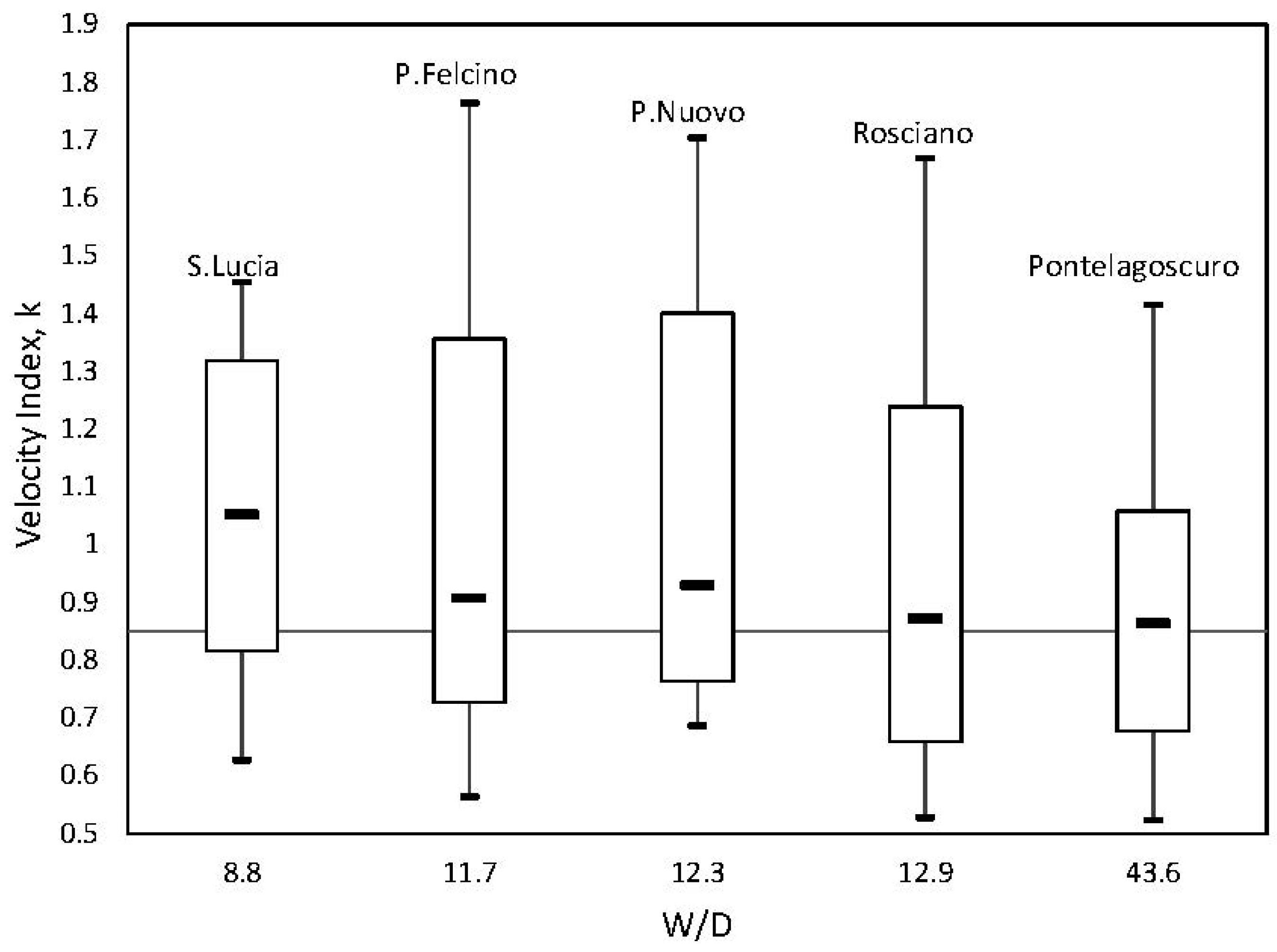
The velocity at the water surface sampled by the current meter is used to mimic the surface velocity measured by SVR or LSPIV. It is worth noting that the analysis does not aim to show the capabilities of the above two technologies but only to verify the relationship between surface velocity and depth-averaged velocity, which is useful to estimate the mean flow velocity by using the velocity-area method. Figure 2 shows the box-plot of the velocity index values for the five gage sites as a function of the aspect ratio, W/D, in terms of the 5th and 95th percentile along with the median, minimum, and maximum values. As can be seen, the velocity index is quite scattered at each gage site, while the median value is inversely proportional with the aspect ratio, starting from 1.05 at Santa Lucia, the narrowest river section, and dropping to 0.86 at Pontelagoscuro, the widest site. Therefore, the average value of the k index observed for the five river gage sites deviates from the constant value of 0.85 used in the literature (e.g., [6,7]); for the Po River the mean value is close to 0.85. It is worth nothing that k > 1 means the dip phenomenon is significant in the velocity profile, causing a consistent curved shape approaching a parabolic one and leading to the depth-averaged velocity being greater than the surface velocity.
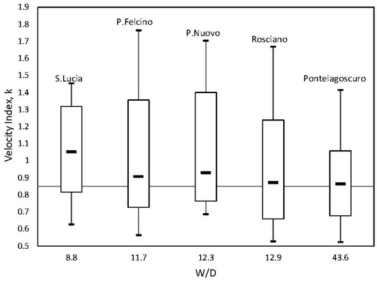
Figure 2.
Box-plot of the values of the velocity index, k, as a function of the aspect ratios, W/D, for the five gage sites based on the velocity dataset. The line corresponding to the value of 0.85 is also shown along with the name of the gage sites.
Moreover, inspecting Figure 2, one infers that the velocity index is also influenced by the geometry of the river site, such as expressed by the aspect ratio, and while the median value tends to decrease for large aspect ratios (e.g., Pontelagoscuro site with W/D = 43.6), the distribution of the velocity index is always scattered, even in the widest channel. Indeed, as can be inferred from Figure 2, the mean value of k tends to be 0.85 for large values of the aspect ratio, while the variance seems to decrease only for the largest W/D occurring at the Pontelagoscuro site.
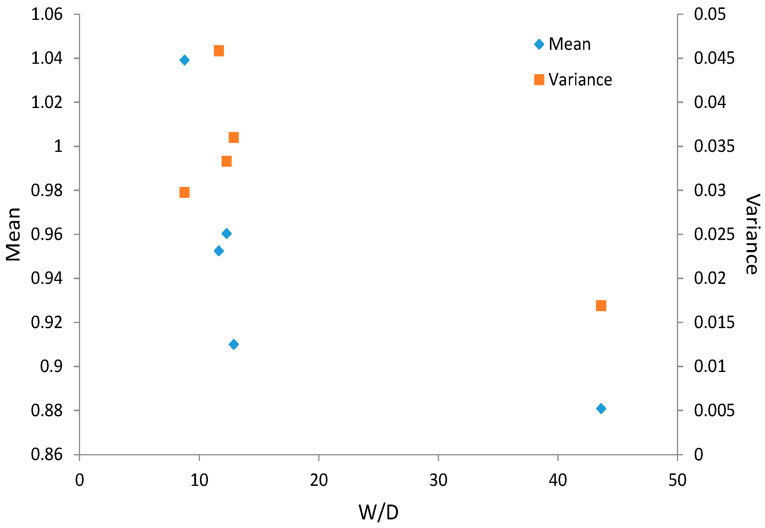
It has to be stressed that the limited sample of river gage sites does not allow a general rule for applying the velocity index to any river worldwide to be inferred. However, Figure 3 provides useful insights into understanding why k = 0.85 cannot be considered a parameter to be applied to rivers everywhere and for whatever flow condition.
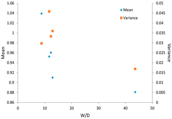
Figure 3.
Mean and variance of the velocity index, k, for the selected gage sites as a function of the aspect ratio (W/D).
At a first attempt, Figure 3 could be useful for addressing the uncertainty in estimating the velocity index as a function of W/D. In this case, identifying the relationship expressing kmean and kvariance as a function of (W/D) could be of support in understanding the variability of the velocity index and, hence, to evaluate how much the depth-averaged velocity can vary at each vertical sampled in correspondence to the surface velocity measurement. However, more gage sites are necessary to identify a robust relationship that can be leveraged in addressing the uncertainty in the k estimation.
Therefore, the above results indicate that, by using new technologies as SVR and/or LSPIV, the application of a velocity index when dip phenomena occur may affect the accuracy of the mean flow velocity assessment and, hence, of the discharge.
4.2. Comparison of Depth-Averaged Velocities
Based on the previous analysis, it is evident that the assumption of a constant index velocity, i.e., 0.85, might lead to an incorrect estimate of the depth-averaged velocity and, hence, of the discharge. The variability of the index velocity for each vertical sampled in the cross-sectional flow area depends on the presence of dip phenomena due to effect of secondary currents caused by side walls, bridges, and wind effects, as well as the presence of floating material. These effects seem to tend to be smooth for large values of the aspect ratio. Therefore, in the case of streamflow measurements the use of the velocity index method should be applied with care and the reliability verified.
The entropy method proposed here allows the location of the maximum velocity below the water surface (dip) for each vertical sampled in the flow area to be estimated, starting from the measured surface velocity. The procedure illustrated in Figure 1 is applied for all measurements available at the selected gage sites and the results are compared with the ones obtained using the velocity index method with k = 0.85.
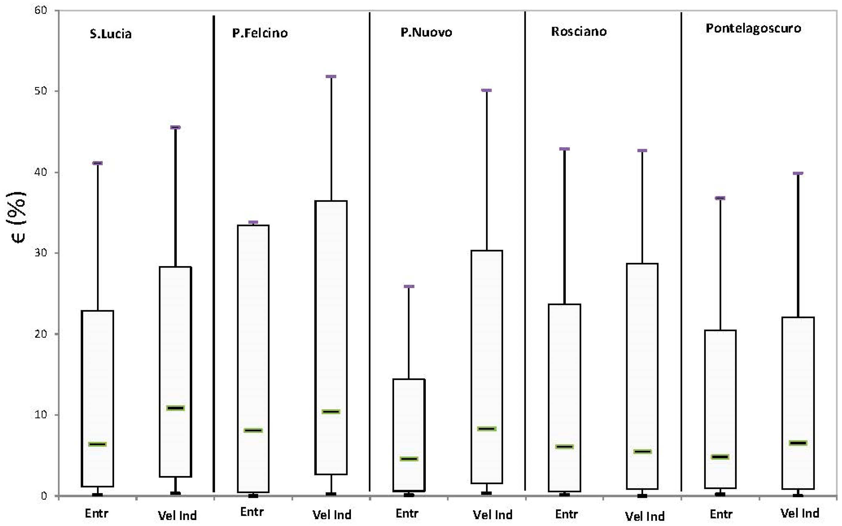
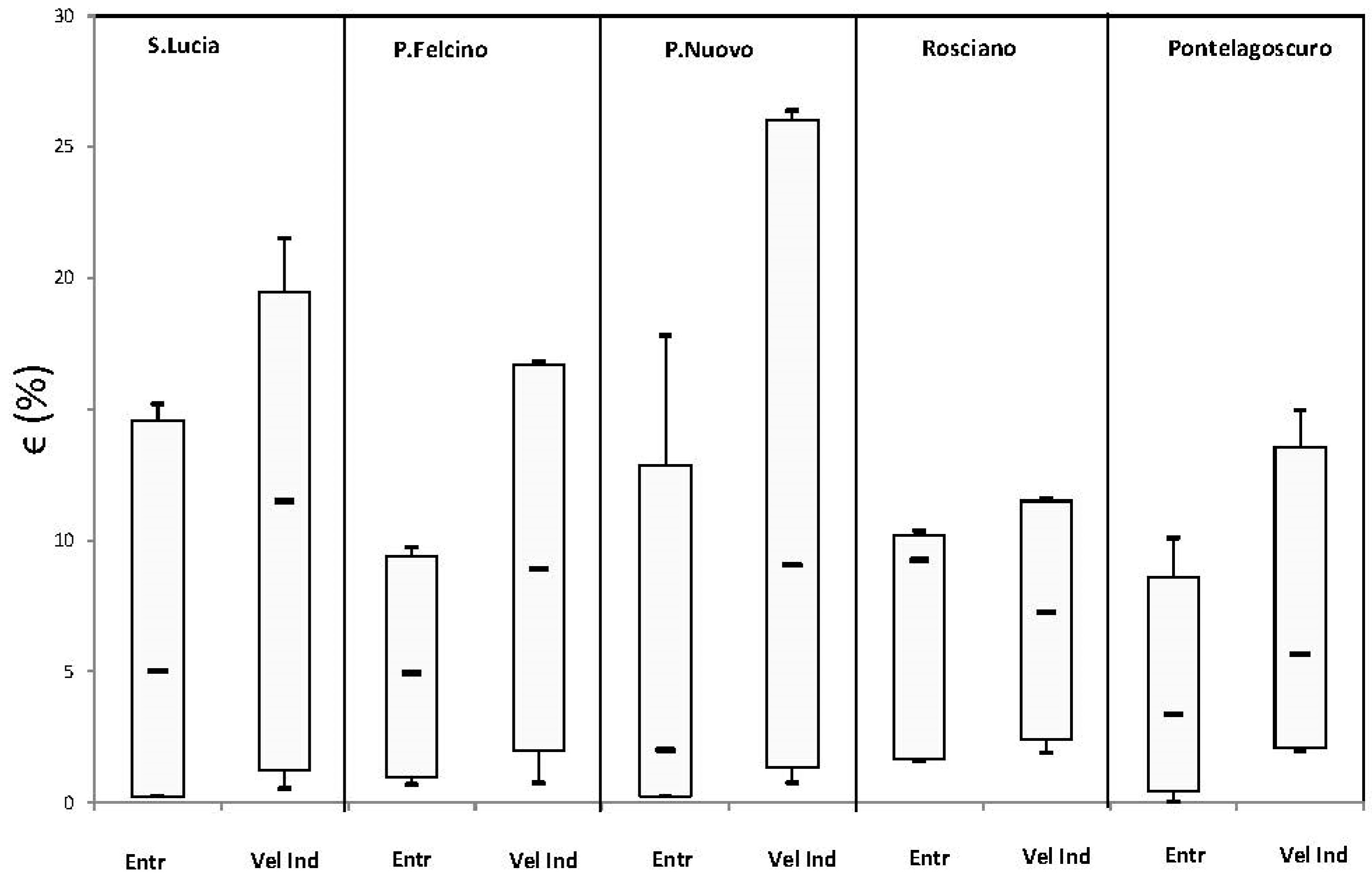
To this end, the error in magnitude for the depth-averaged velocity is computed for each gage sites and the results are shown in Figure 4 in terms of a box-plot referring to the median, 5th, and 95th percentile. As can be seen and expected, the differences are more noticeable for the narrower gage sites, with a median that does not exceed 6% and 11% for the entropy and the velocity index method, respectively; while for the Pontelagoscuro site, the differences are less evident, even though a slightly larger scatter is always present in the velocity index approach.
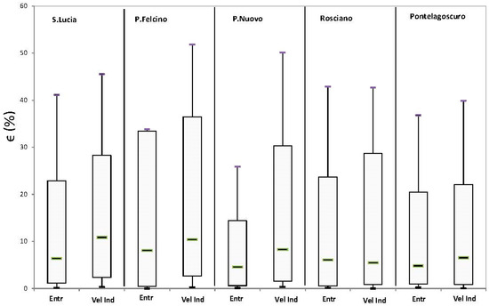
Figure 4.
Box-plot of absolute percentage errors () in estimating the depth-averaged velocity using the entropy approach (Entr) and the velocity index (Vel Ind).
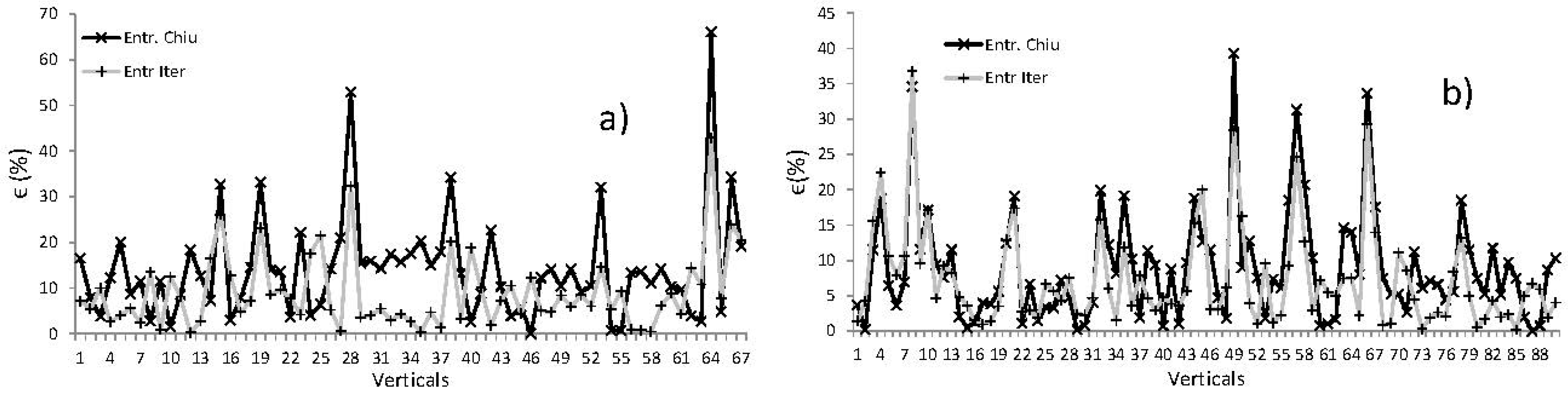
The entropy approach has been also compared with Chiu and Tung’s formulation [24], for which the dip is computed without an iterative procedure. In this case, the dip computed by Equation (7) is replaced in Equation (3), from which is computed and used in Equation (1). By way of example, Figure 5 shows for the Rosciano and Pontelagoscuro gage sites the comparison between the errors in depth-averaged velocity computed using the dip assessment by [25] and the proposed iterative method. As can be seen, the iterative entropy approach performs better than the one based on Chiu’s dip, and, as expected, the difference tends to decrease if the aspect ratio increases as for the Pontelagoscuro site. Similar performances obtained at the Rosciano site are for the three sites with lower aspect ratios (W/D). Table 2 shows the mean and standard deviation of the percentage errors in magnitude of estimating the depth-averaged velocity by using Equation (7) and the method proposed here for the dip assessment, showing again that the dip computed by the iterative procedure is more accurate than that based on Equation (7).

Figure 5.
Absolute percentage error in estimating the depth-averaged velocity using the dip assessment by the iterative procedure proposed here (Entr Iter) and Chiu’s formula (Entr Chiu) for (a) the Rosciano and (b) the Pontelagoscuro gage sites.
Table 2.
Mean and standard deviation of the absolute percentage error in estimating the depth-averaged velocity using the dip assessment by the iterative procedure proposed here (Entr Iter) and Equation (7) (Entr Chiu) for the investigated gage sites.
4.3. Comparison of Mean Flow Velocity and Discharge
Once the depth-averaged velocities are computed for each measurement, the cross-sectional mean flow velocity can be estimated using the velocity-area method. Considering that the estimate of dip across the flow area by the proposed approach is more robust than that based on Equation (7), the analysis is here addressed for the proposed procedure and velocity index only.
Figure 6 shows the box-plot of the absolute percentage error in the computation of mean flow velocity for the whole velocity dataset for the five investigated gage sites. As can be seen, the entropy approach performs better than the velocity index one, as is inferable by comparing the median and 95th percentile of errors and the differences in terms of the median and scattering tend to smooth for larger aspect ratios, as for the Rosciano and Pontelagoscuro gage sites. The mean percentage error does not exceed 4.5% and 10% for the entropy and velocity index methods, respectively.
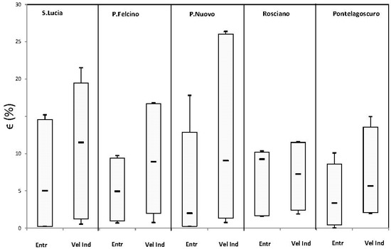
Figure 6.
Box-plot of the absolute percentage error () in estimating the cross-sectional mean flow velocity using the Entropy approach (Entr) and the velocity index (Vel Ind).
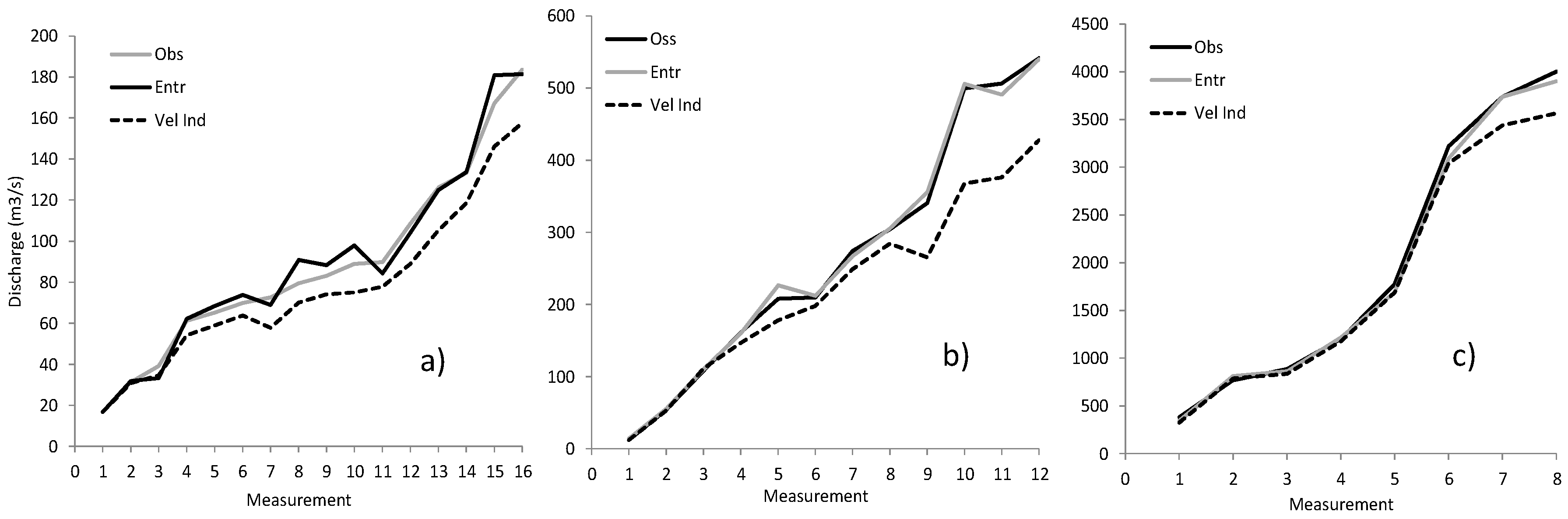
Moreover, considering the performances of the two methods the greatest differences are identified for higher mean flow velocity, as can be seen in Figure 7, where a comparison between the observed discharge and the one computed by the entropy and velocity index approaches is shown for the Santa Lucia, Ponte Nuovo, and Pontelagoscuro gage sites. Similar results are found for Ponte Felcino and Rosciano. Figure 7 demonstrates that, for the velocity index method (k = 0.85), the maximum errors shown in the graph in Figure 6 are referred to as the high discharges with an error greater than 26%. This proves that the velocity index method needs to be applied with care if high flood events are of interest. Conversely, for the proposed entropy approach the maximum error in percentage is obtained for the lower flows and does not exceed 14%, while for high floods the errors do not exceed 3%, thus showing the benefit in using the method for the monitoring of high floods starting from the sampling of surface flow velocity.
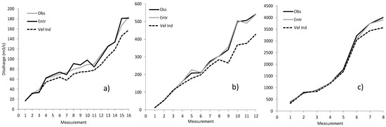
Figure 7.
Comparison between observed discharge (Obs) and discharge computed by the Entropy approach (Entr) and the velocity index (Vel Ind) for (a) Santa Lucia; (b) Ponte Nuovo; and (c) Pontelagoscuro.
Finally, the correlation between umaxv values observed and computed by the entropy method for each vertical is found good with the coefficient of determination, R2, varying from 0.84 for the narrower sites (Santa Lucia and Ponte Felcino) to 0.94 for the wider ones. Moreover, by way of example, Figure 8 shows for the highest flood in the dataset of the Ponte Nuovo gauged site, the comparison between the velocity profile at four different verticals computed by the entropy method, and the velocity points sampled by current meter. It is worth noting that the velocity profiles are obtained just by sampling usurf, and no information is used in terms of dip. It is noticeable how the velocity profile shape computed by Equation (1) is able to embed the observed points and, particularly, umaxv. Similar performances are obtained for the velocity dataset of the other investigated gage sites.
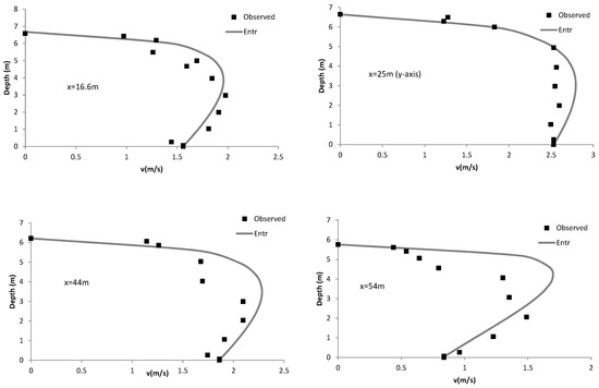
Figure 8.
Velocity profiles estimated by entropy method (Equations (1) and (5)) plotted against velocity points sampled by current meter along four verticals during the highest flood of the velocity dataset at the Ponte Nuovo gage site. x is the distance from the left bank, while the y-axis represents the vertical where umax occurs.
5. Conclusions
The trialing of emerging no-contact technologies, like SVR and LSPIV, for surface flow velocity measurement in rivers is of considerable interest and represents an effective alternative to conventional monitoring. These new technologies allow the issues related to the limited availability of hydraulic information due to low flow conditions and the difficulties and dangers to operators measuring velocity points in the lower portion of flow area using standard sampling techniques to be overcome.
In this context, this work addresses the crucial matter of turning the surface velocity into depth-averaged velocity, even if secondary current effects occur, for whatever natural channel geometry, providing some useful insights.
Based on the field data used, it has been shown that the proposed entropic algorithm well lends itself to being applied when advanced no-contact technology is used to estimate the discharge by monitoring the surface flow velocity across the river. The dip phenomenon, having a fundamental role in depth-averaged velocity assessment, is accurately identified by the entropy procedure for whatever flow conditions at the investigated gage sites.
The velocity index method, with k = 0.85, is of little use for rivers with a lower aspect ratio, with significant errors in estimating high discharges; while for wider rivers, its performance is found quite similar to that of the entropy method, considering that the dip phenomena are quite negligible. The relationship found between the mean and variance of the aspect ration of the k index needs to be further investigated by extending the velocity dataset and the case studies.
Acknowledgments
This work was partly funded by The Project of Interest NextData (MIUR-CNR). The authors wish to thank the Umbria Region Department of Environment, Planning, and Infrastructure, for providing Tiber River basin data. The authors want to thank Cristiano Corradini for the technical support. Finally, the Reviewers are gratefully acknowledged for their useful comments.
Author Contributions
All authors contributed extensively to the work. Tommaso Moramarco developed the methodology, conceived and performed the numerical experiments, and wrote the article. Silvia Barbetta and Angelica Tarpanelli contributed equally to the discussion of methodology, results analysis and the manuscript writing.
Conflicts of Interest
The authors declare no conflict of interest.
References
- Moramarco, T.; Saltalippi, C.; Singh, V.P. Velocity profiles assessment in natural channel during high floods. Hydrol. Res. 2011, 42, 162–170. [Google Scholar] [CrossRef]
- Di Baldassarre, G.; Montanari, A. Uncertainty in river discharge observations: A quantitative analysis. Hydrol. Earth Syst. Sci. 2009, 13, 913–921. [Google Scholar] [CrossRef]
- Muller, G.; Bruce, T.; Kauppert, K. Particle image velocimetry: A simple technique for complex surface flows. In Proceedings of the International Conference on Fluvial Hydraulics, Balkema, Lisse, The Netherlands, 4–6 September 2002; pp. 1227–1234.
- Simpson, M.R.; Oltman, R.N. Discharge Measurement System Using an Acoustic Doppler Current Profiler with Applications to Large Rivers and Estuaries: U.S. Geological Survey Water-Supply Paper 2395; U.S. Geological Survey: Reston, VA, USA, 1993; 32p.
- Wagner, C.R.; Mueller, D.S. Comparison of bottom-track to global positioning system referenced discharges measured using an acoustic Doppler current profiler. J. Hydrol. 2011, 401, 250–258. [Google Scholar] [CrossRef]
- Costa, J.E.; Spicer, K.R.; Cheng, R.T.; Haeni, F.P.; Melcher, N.B.; Thurman, E.M. Measuring stream discharge by non-contact methods: A proof-of-concept experiment. Geophys. Res. Lett. 2000, 27, 553–556. [Google Scholar] [CrossRef]
- Welber, M.; Le Coz, J.; Laronne, J.B.; Zolezzi, G.; Zamler, D.; Dramais, G.; Hauet, A.; Salvaro, M. Field assessment of noncontact stream gauging using portable surface velocity radars (SVR). Water Resour. Res. 2016, 52, 1108–1126. [Google Scholar] [CrossRef]
- Fujita, I.; Muste, M.; Kruger, A. Large-scale particle image velocimetry for flow analysis in hydraulic applications. J. Hydraul. Res. 1998, 36, 397–414. [Google Scholar] [CrossRef]
- Tauro, F.; Porfiri, M.; Grimaldi, S. Orienting the camera and firing lasers to enhance large scale particle image velocimetry for streamflow monitoring. Water Resour. Res. 2014, 50, 7470–7483. [Google Scholar] [CrossRef]
- Muste, M.; Fujita, I.; Hauet, A. Large-scale particle image velocimetry for measurements in riverine environments. Water Resour. Res. 2008, 44. [Google Scholar] [CrossRef]
- Ferro, V. ADV measurements of velocity distributions in a gravel-bed flume. Earth Surf. Proccess. Landf. 2003, 28, 707–722. [Google Scholar] [CrossRef]
- Dingman, S.L. Probability Distribution of Velocity in Natural Channel Cross Sections. Water Resour. Res. 1989, 25, 509–518. [Google Scholar] [CrossRef]
- Yang, S.Q.; Tan, S.K.; Lim, S.Y. Velocity distribution and dip-phenomenon in smooth uniform open channel flows. J. Hydraul. Eng. 2004, 130, 1179–1186. [Google Scholar] [CrossRef]
- Chiu, C.L. Application of Entropy Concept in Open-Channel Flow Study. J. Hydraul. Eng. 1991, 117, 615–627. [Google Scholar] [CrossRef]
- Singh, V.P.; Fontana, N.; Marini, G. Derivation of 2D power-law velocity distribution using entropy theory. Entropy 2013, 15, 1221–1231. [Google Scholar] [CrossRef]
- Fontana, N.; Marini, G.; De Paola, F. Experimental assessment of a 2-D entropy-based model for velocity distribution in open channel flow. Entropy 2013, 15, 988–998. [Google Scholar] [CrossRef]
- Corato, G.; Moramarco, T.; Tucciarelli, T. Discharge estimation combining flow routing and occasional measurements of velocity. Hydrol. Earth Syst. Sci. 2011, 15, 2979–2994. [Google Scholar] [CrossRef]
- Chiu, C.L. Velocity distribution in open channel flow. J. Hydraul. Eng. 1989, 115, 576–594. [Google Scholar] [CrossRef]
- Moramarco, T.; Saltalippi, C.; Singh, V.P. Estimation of mean velocity in natural channel based on Chiu’s velocity distribution equation. J. Hydrol. Eng. 2004, 9, 42–50. [Google Scholar] [CrossRef]
- Farina, G.; Alvisi, S.; Franchini, M.; Moramarco, T. Three methods for estimating the entropy parameter M based on a decreasing number of velocity measurements in a river cross-section. Entropy 2014, 16, 2512–2529. [Google Scholar] [CrossRef]
- Moramarco, T.; Singh, V. Formulation of the entropy parameter based on hydraulic and geometric characteristics of river cross sections. J. Hydrol. Eng. 2010, 15, 852–858. [Google Scholar] [CrossRef]
- Fulton, J.; Ostrowski, J. Measuring real-time streamflow using emerging technologies: Radar, hydroacoustics, and the probability concepts. J. Hydrol. 2008, 357, 1–10. [Google Scholar] [CrossRef]
- Herschy, R.W. Streamflow Measurement; Elsevier: London, UK, 1985. [Google Scholar]
- Corato, G.; Melone, F.; Moramarco, T.; Singh, V.P. Uncertainty analysis of flow velocity estimation by a simplified entropy model. Hydrol. Process. 2014, 28, 581–590. [Google Scholar] [CrossRef]
- Chiu, C.-L.; Tung, N.-C. Maximum velocity and regularities in open-channel flow. J. Hydraul. Eng. 2002, 128, 390–398. [Google Scholar] [CrossRef]

© 2017 by the authors. Licensee MDPI, Basel, Switzerland. This article is an open access article distributed under the terms and conditions of the Creative Commons Attribution (CC BY) license ( http://creativecommons.org/licenses/by/4.0/).