1. Introduction
Evapotranspiration (ET) is one of the major processes in the hydrologic cycle and plays an essential role in controlling energy and water exchanges between the land surface and the atmosphere. ET is also a key component in water resource management across multiple scales for agricultural and ecological applications [
1]. ET is the summation of evaporation and transpiration, which consume water to different degrees in areas with different land cover types; thus, this parameter is significantly affected by the land-surface characteristics.
Given the dwindling supplies of available water resources due to over-withdrawal of groundwater and water pollution, water resource management has shifted from traditional large-scale approaches to approaches that rely on ET to estimate temporal changes, which concentrate to a greater degree on identifying temporal changes and the spatial distribution of water consumption, especially in intensely irrigated farming areas [
2]. Furthermore, the results of water-saving techniques, such as drip irrigation and sprinkler irrigation, could be monitored using ET data, thus improving water-use efficiency (WUE) and enhancing the ability of farmers to efficiently manage available irrigation water supplies [
3,
4,
5,
6].
Gridded ET from remote sensing (RS)-based methods, however, suffers from the temporal and spatial limitations from RS sensors. For example, Moderate Resolution Imaging Spectroradiometer (MODIS) products (which have a spatial resolution of 1 km) can be obtained twice daily, and approximately 100 images are available each year after the images influenced by clouds are removed. In contrast, only one Landsat8 image with a resolution of 30 m is taken every 16 days, regardless of cloud cover. Consequently, trade-offs exist between different RS-based methods, and combinations of different ET datasets and methods are required to improve the success of water resources management [
7].
Given the limitations of RS images, a combination of images from diverse sensors can be used to obtain a complete time series of stable and higher-resolution gridded ET data. Martha C. Anderson interpolated ET snapshots obtained at the time of clear-sky Landsat overpasses [
8]. In this work, the ratio of actual ET to a reference ET (fRET) obtained from Landsat data after spline interpolation, ALEXI fRET data obtained by applying the Savitsky–Golay filter [
9], and daily meteorological data were used as inputs. Similarly, many methods employ actual ET (ETa) and potential ET from cloud-free days and assume that the ratio of fRET or the evaporative fraction (EF) is the same or changes in an orderly fashion. Such methods include the reference ET fraction [
10,
11,
12,
13], Todorovic [
14,
15,
16], and evaporative fraction [
17,
18] methods. For Landsat8 data, the effects of clouds and the satellite repeat interval both contribute to image-sparse areas. Traditional temporal gap-filling methods may filter out some high-frequency signals, such as irrigation, during these long time intervals.
Another approach involves downloading coarser-scale datasets that combine the benefits of diverse kinds of remote sensors. Downscaling is defined as an increase in spatial resolution following disaggregation of the original dataset based on fitting a statistical relationship [
19,
20], which requires information at a desired fine resolution [
21,
22,
23]. Liu and Wu used the spatial and temporal adaptive reflectance fusion model (STARFM) to downscale 1-km ETa data [
24]. Yasir H. Kaheil presented an algorithm using the discrete wavelet transform (DWT) and support vector machines (SVMs) to downscale and forecast ET values at a spatial resolution of 15 m, which is similar to the resolution used by Ke [
25,
26]. In addition, the U.S. Geological Survey investigated the downscaling potential of simplified surface energy balance (SSEB)-derived ETa data from 1 km to 250 m by correlating the ET data with Normalized Difference Vegetation Index (NDVI) values from MODIS [
27].
A correlation exists between vegetation and ET. Transpiration through the stomata of plant leaves accounts for the majority of ET, especially in arid and semi-arid areas, due to the low soil moisture content. For example, the study by Zhuang [
28] concluded that the fractional vegetation cover (fvc) and canopy resistance (Rc) retrieved from images displaying NDVI values control the sensible heat flux between the surface and the atmosphere. Additionally, NDVI has also been suggested as a major factor controlling the inter-annual variations in ET over relatively broad scales [
29]. Many studies have highlighted the advantages of using vegetation indices (VIs) to estimate ET in previous decades [
30,
31,
32,
33,
34,
35,
36]. Edward P. Glenn summarized correlation coefficients between ET estimates based on VIs combined with relevant variables and in situ observations [
36].
This study aims to introduce Landsat8 30-m NDVI data as a readily available and applicable source of information on spatial patterns combined with land cover information at the same spatial scale. In addition, regression coefficients determined only over small areas (one MODIS pixel) were employed to downscale the ETa data. Three in situ flux sites in two study areas are then used to compare with the results of the so-called “de-pixelation” method, which disaggregates the ETWATCH 1-km ETa dataset to a resolution of 30 m.
3. Method
In principle, the ETa values within a given coarse pixel (usually a MODIS 1-km pixel) should be nearly the same for homogeneous surface conditions, given that meteorological factors typically remain constant over short distances. However, due to the heterogeneity of the land surface, which contains different land cover types and topography, ET values vary among small patches.
One type of output downscaling that is currently widely used can be called the “correlation” approach. This process uses the relationship between ETa data from two MODIS images (or other high temporal resolution datasets) separated by a given time interval [
7,
23,
57]. To advance this type of strategy by building relationships based on Landsat ET over small areas, in this study, spatial patterns from NDVI data within individual fine pixels are highlighted. Assuming that the 1-km ETa data used in this research provide a good representation of the actual conditions, the following equation can be used:
where
is the downscaled ET result at a resolution of 30 m;
is the ETa calculated from MODIS data at a resolution of 1 km (ETWatch in this research); and
and
are driving factors calculated from the 30-m resolution images. Downscaling using this scheme can ensure that the sum of the downscaled ET will be the same as that of the entire coarse pixel.
A monthly 30-m NDVI image is combined with the land cover map at the same spatial resolution to calculate the indicators and . The transpiration associated with vegetation is greater than the evaporation associated with soil during the growing season, and the magnitude of the transpiration varies among different vegetation types. Hence, the historical ratio of NDVI/ETa was used to diminish the potential deviation because of heterogeneity in the land surface.
A lower ratio of NDVI/ETa (usually occurring within cropland) may lead to an increase in the downscaled ET using NDVI only for cropland inside individual mixed 1-km pixels. Therefore, the NDVI obtained directly from Landsat8 must be modified to eliminate this deviation. The relevant equation can be written as follows:
where
is the factor that offsets the NDVI due to the different NDVI/Eta ratios, which depend on the land cover type
i and the month
m.
is the average NDVI value for land cover type
i and month
m,
is the average ET value for land cover type
i and month
m, and
is the summation of NDVI/ET for all land cover types in month m. In Equation (3),
is the downscaling indicator used in Equation (1),
is derived from satellite data from month
m, and
is the offset factor in Equation (2) for month m. In this strategy, a lower ratio of NDVI/ETa leads to a lower offset factor of
Ra within a given area. This difference may lead, in turn, to a lower fine-scale ET value compared with the NDVI-downscaled result because the offset was added to the NDVI. This effect is especially pronounced within mixed pixels.
This study assumes that the vegetation conditions described by the NDVI do not change greatly within individual months. Thus, monthly NDVI information is used to represent the spatial pattern of the land surface and estimate the ten-day ET. Therefore, ten-day 30-m ET data can be obtained at the same temporal scale as the 1-km ETa data with the following model, which is similar to Equation (1):
where
and
are the monthly NDVI data after offsetting them by
Ra;
represents the ten-day 30-m ET data; and
represents the ten-day 1-km ET data in a given month. A ten-day temporal interval is chosen because a ten-day period is close to the 8-day sampling interval of the MODIS evapotranspiration product (MOD16). In addition, ten-day data can easily be converted into 30-day data, which agrees with the sampling frequency of the NDVI data source.
Given the needs of water resource management for data on cropland in particular areas and to meet the demand for data high temporal and spatial resolutions, the evaluation of the downscaling method is performed in terms of accuracy using in situ data (EC) and in terms of consistency with the original ETWATCH ETa dataset in the following section.
4. Results
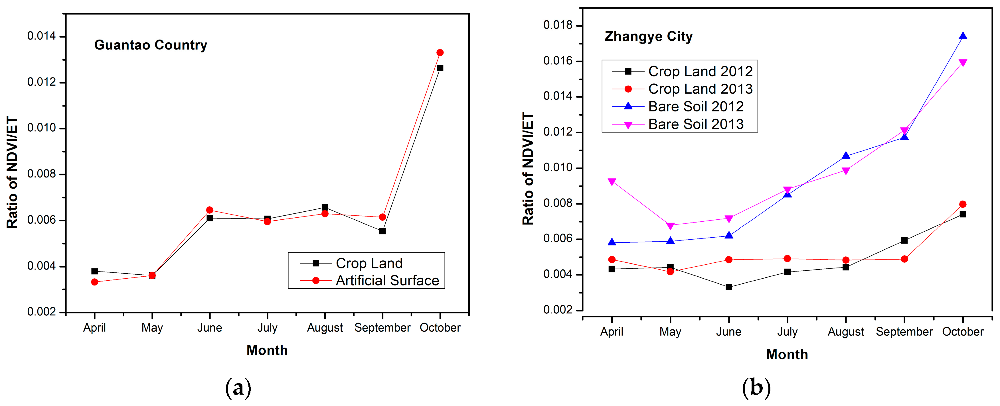
In this research, the ratio of historical NDVI/ETa was calculated from the original 1-km dataset. Differences exist among the different land cover types; however, these differences remain stable over time (2012–2013 in the Heihe Basin). Comparisons of the ratios of the two main land cover types in the two study areas are provided in
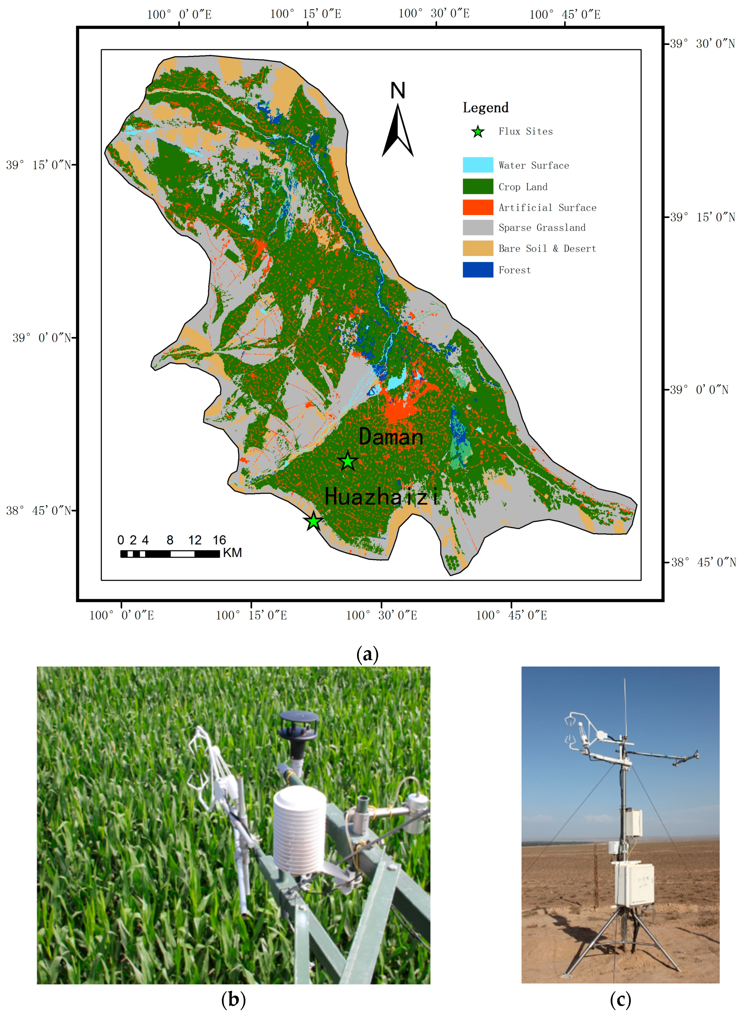
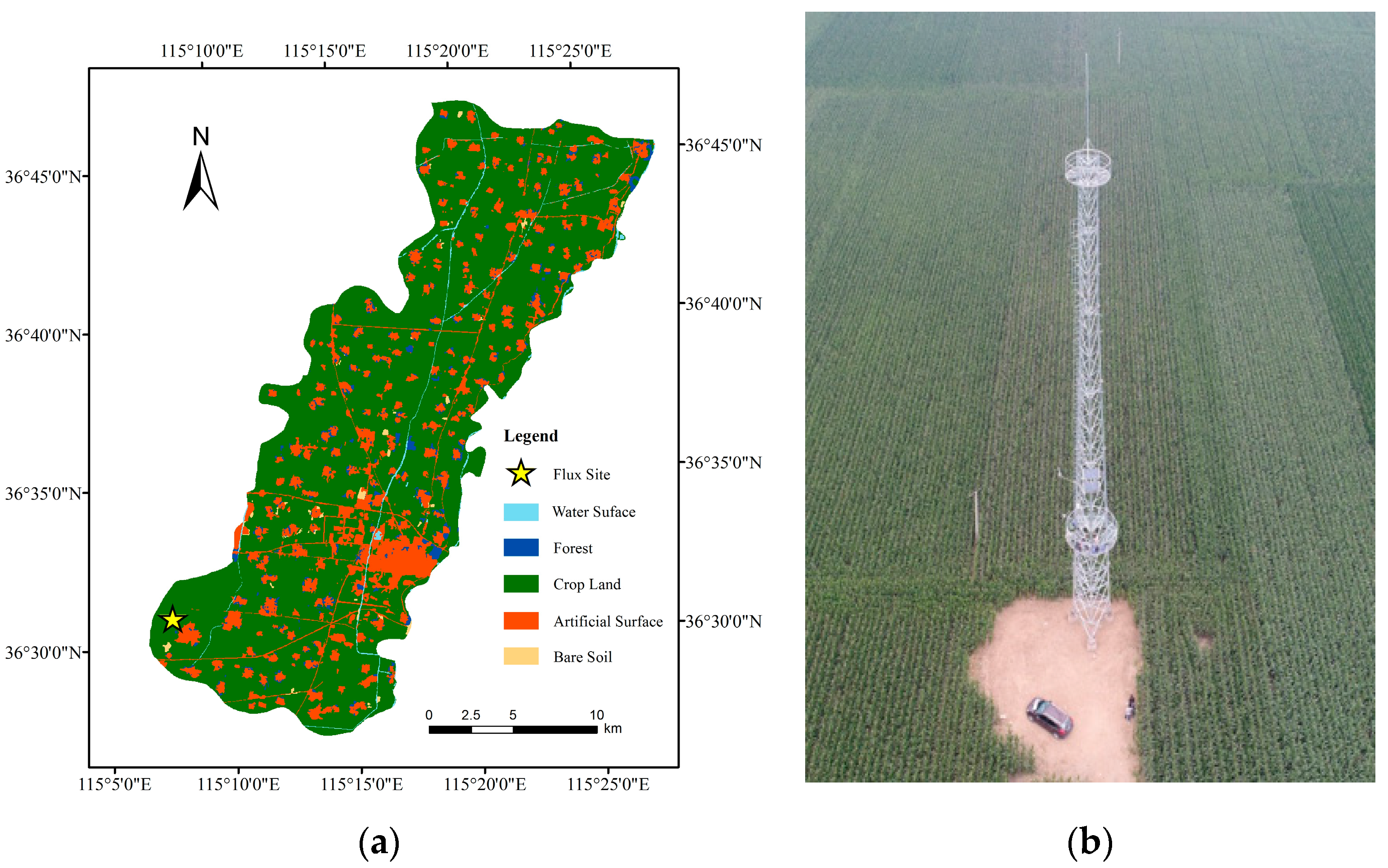
Figure 3. Based on these comparisons, the differences are more obvious in Zhangye City than in Guantao County because Zhangye is an oasis that relies on irrigation and is surrounded by desert and bare soil. Thus, the water consumption of Zhangye cropland differs from that of the surrounding plant-sparse area. However, the difference diminished considerably in the semi-moist area, where precipitation is relatively abundant. These favourable moisture conditions ensure the growth of green plants in towns and villages, leading to a small difference between the NDVI and ETa values for the cropland.
A lookup table for the Ra values calculated based on ETWatch data in the two study areas is provided in
Table 5. Only two main land cover types were considered in Guantao County because cropland and artificial surfaces together occupy over 95% of the entire county; thus, other types were ignored in this study. Therefore, the NDVI values in areas of forest, bare soil and water are not modified.
Using the Ra lookup table above, 1-km ET was then decomposed into 30-m ET for the two regions in 2013 with a ten-day time interval.
Figure 4 shows the spatial distribution of the downscaled results and the ETWatch 1-km ETa map for the entire growing season (interpolated to the same resolution). The downscaled results show good spatial consistency with the original ETWatch coarse data. There is a valley in the northeast of the middle section of the Heihe Basin (
Figure 4a,b). The ET in the valley is relatively higher due to the efficient water supply. This tendency is reflected in the downscaled result. Finer-scale details, such as highways and field patches, can be recognized in the downscaled map as well. This phenomenon is more obvious in Guantao Country. A small village in this region surrounded by cropland is shown in the downscaled map but is obscure in the coarse map. The spatial patterns provided by Landsat images are therefore suitable for downscaling.
4.1. Comparison with the Original ETWATCH Dataset
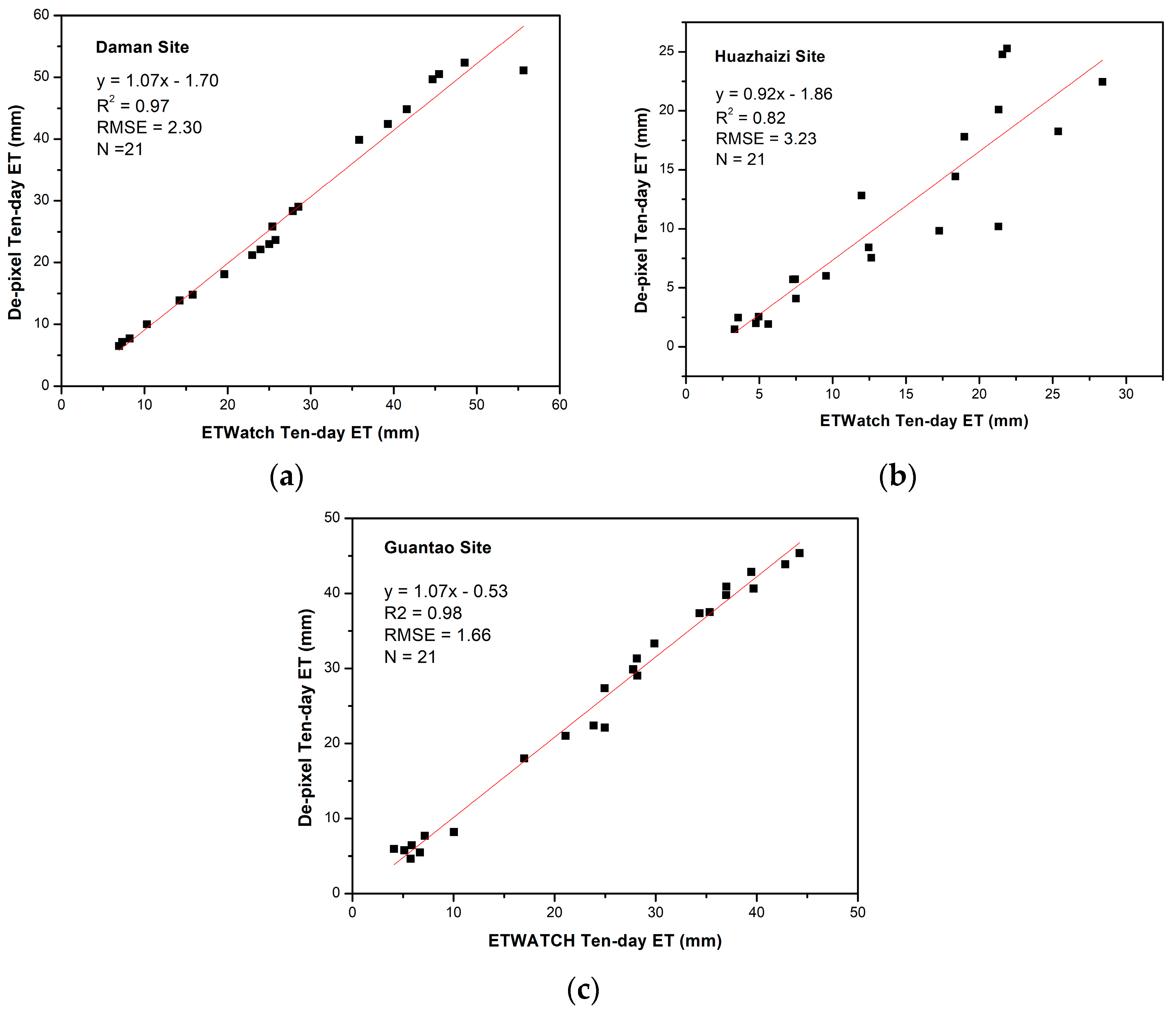
Downscaled ET values over all three sites show good agreement with the original ETWATCH dataset (
Figure 5). The R
2 values resulting from this comparison range from approximately 0.98 at Daman (DM) and Guatntao (GT) to 0.82 at Huazhaizi (HZZ). This good agreement demonstrates that the accuracy of the downscaled dataset depends primarily on the quantity of coarse ETa data available, especially within relatively homogeneous areas. Considering that many of the crop fields in the study area are relatively homogenous (i.e., not many sparsely distributed, fine-scale crop pixels are present) and have similar NDVI values, this good agreement is consistent with our expectations. The smallest R
2 value and the lowest degree of temporal agreement are obtained for site HZZ because of the irregular distribution of bare soil, rock and plants near the site, resulting in abrupt changes in the NDVI (site HZZ lies within a sparse grassland that is located 150 m from a sand-covered area and 800 m from cropland).
The analysis given above suggests that the accuracy of the fine dataset after the “de-pixelation” method depends strongly on the coarse ETa data because of the high degree of correlation, especially within homogenous areas, and partly on the complexity of the land surface. Generally, lower vegetation cover fractions and more complex land cover distributions result in lower accuracy.
4.2. Validation Using In Situ Observation
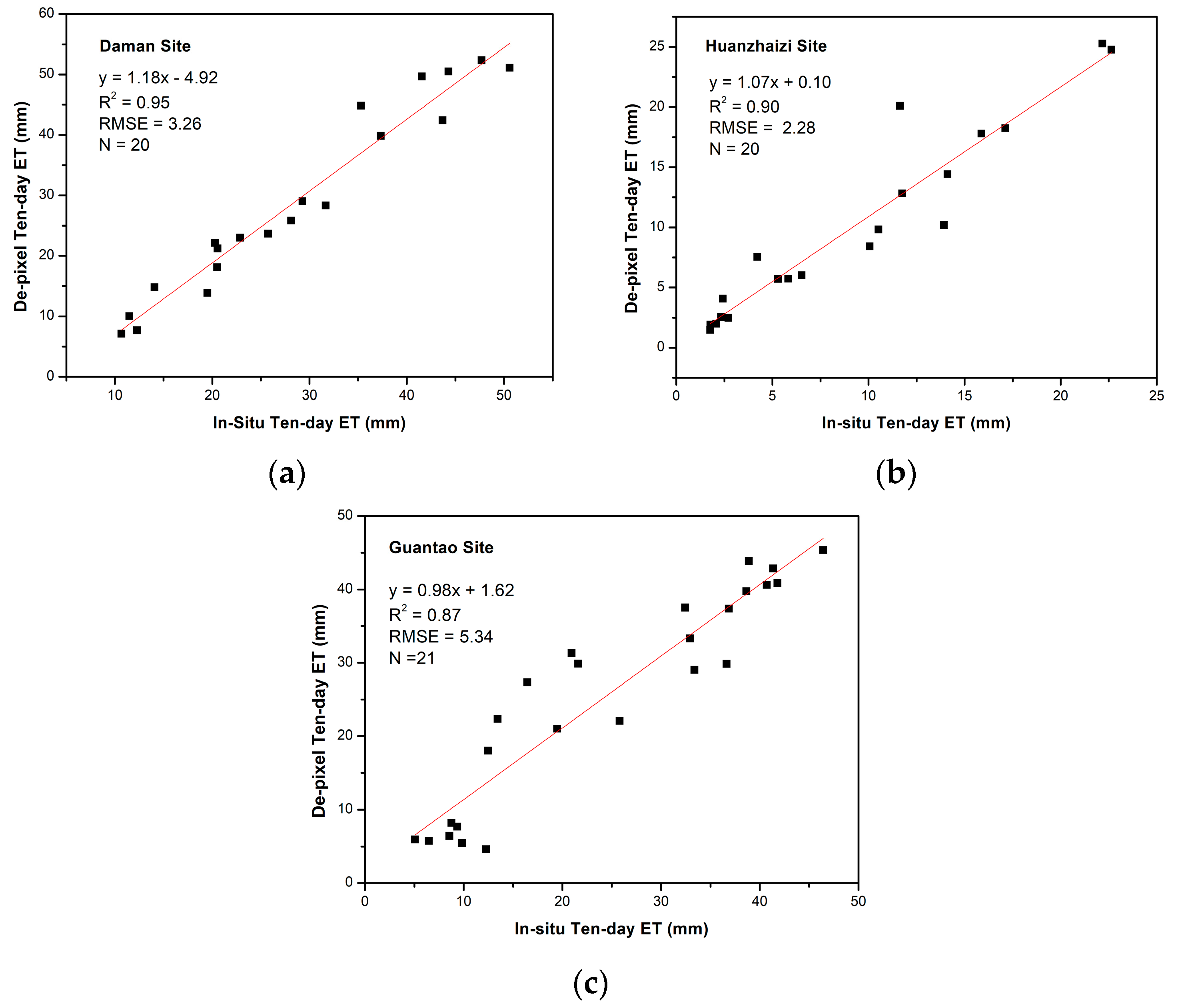
The ten-day dataset obtained by applying the “de-pixelation” method at three flux sites (DM, HZZ and GT), as summarized in
Section 2.1, has been extracted for comparison with the in situ observations. The ET results obtained after “de-pixelation” for all three sites show good agreement with the in situ data, whereas the R
2 values range from 0.87 (GT) to 0.95 (DM) and the RMSE ranges from 2.28 (HHZ) to 5.34 (GT) per ten-day interval (
Figure 6). The model performs well, especially at the HZZ and DM sites (after eliminating one abnormal EC record of 33 mm in the first ten-day period of April, which contrasts with the values of only 10 mm obtained for the other two ten-day periods in the same month). The model also performs well at the GT site, which is positioned within a relatively uniform crop field. Maize is planted at the DM site, and two-season crops are planted at the GT site. Compared with the other two sites, the HZZ site shows little overestimation of the ET values compared with the observations (
Figure 7). Therefore, the “de-pixelation” model displays better performance within crop fields with relatively broad and homogeneous areas than in areas of bare soil and sparse vegetation.
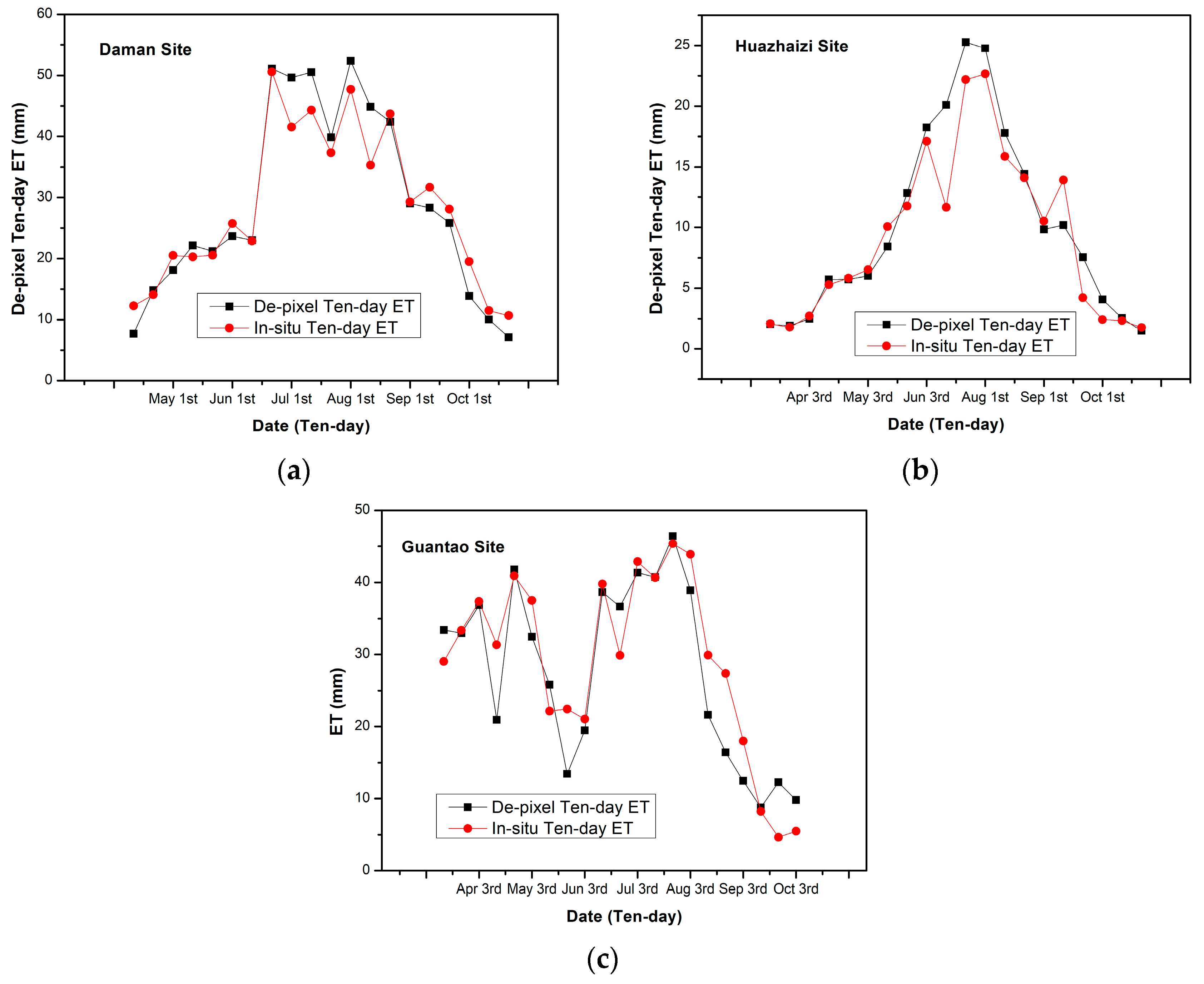
A comparison of the 1-km dataset and the 30-m product with the in situ observations is shown in
Table 6. At all three sites, the 30-m dataset shows good consistency, in terms of its R
2 value, when compared with the original 1-km product. This finding agrees well with the conclusion given in
Section 4.1, which states that the downscaled dataset strongly resembles the original coarse dataset. The progression of the time series effectively captures the different trends (one seasonal crop at the DM site, a similar trend at the HZZ site but without crop cover, and two seasonal crops with two peaks in the ET curve at the GT site). Little improvement was observed at Huazhaizi Site. The reason is mainly because the mixing of coarse data was decomposed by 30-m surface information.
4.3. Comparison among the Results from Different Data Sources
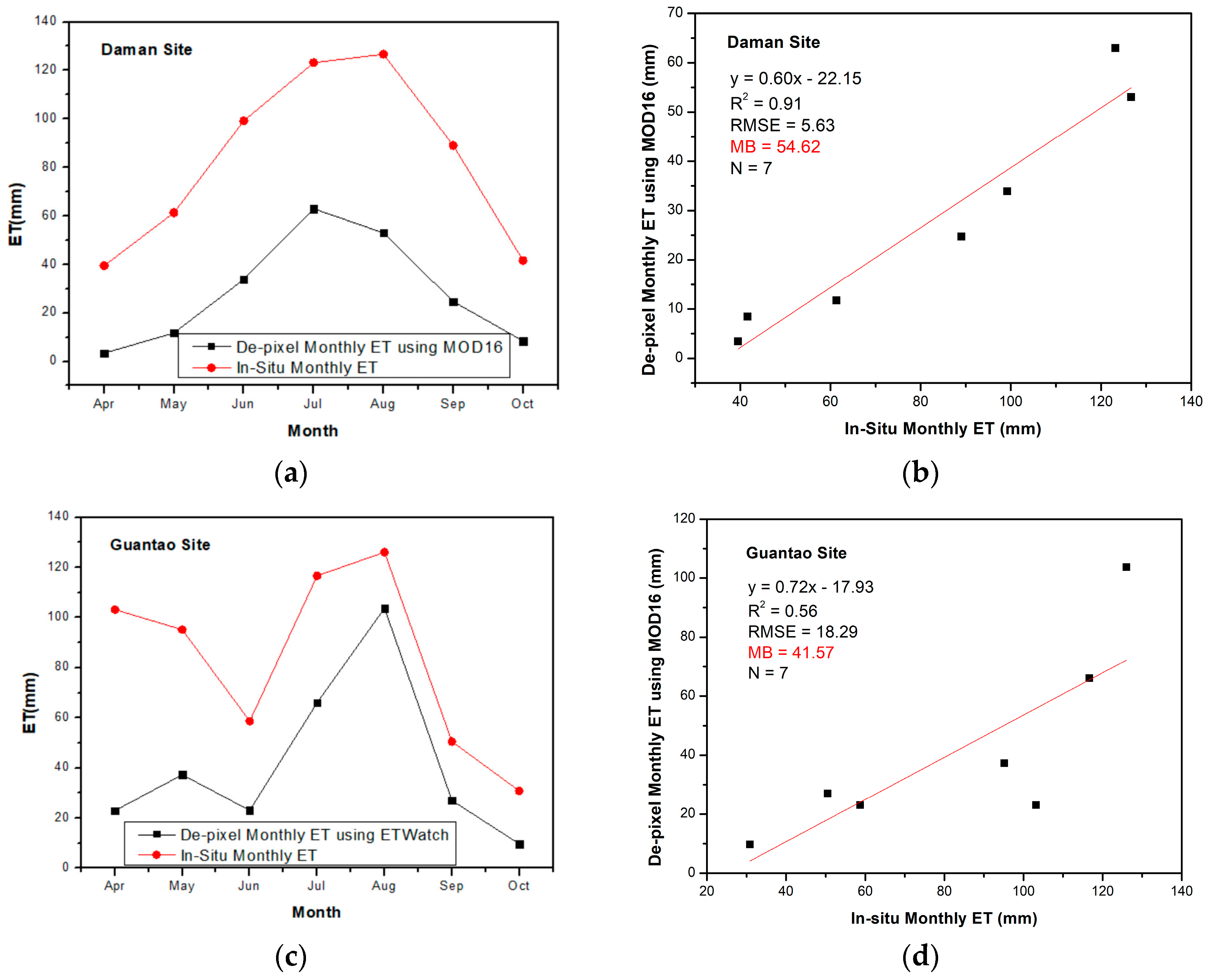
There are two types of input data in the downscaling model, coarse ETa (1 km) and fine NDVI data (30 m). In this section, to evaluate the performance of the “de-pixelation” method under different data-input circumstances, MOD16A2 monthly ETa data are combined with 30-m NDVI data for use in the same downscaling experiment as the ETWatch data. Comparisons of the scatter and progression are shown in
Figure 7. The analysis was not performed for the HZZ site because MOD16A2 data did not cover the bare soil type at this site.
Due to the presence of cloud cover, this analysis used HJ images, which have a revisit period of two days, as a substitute for the Landsat8 data in Zhangye. The data from these two satellites have the same 30-m spatial resolution. Research on the performance of these two sensors shows a good agreement for the measured reflectances in the red and near-infrared (NIR) bands. Data from these bands are needed to calculate the NDVI, especially within areas of cropland and bare soil [
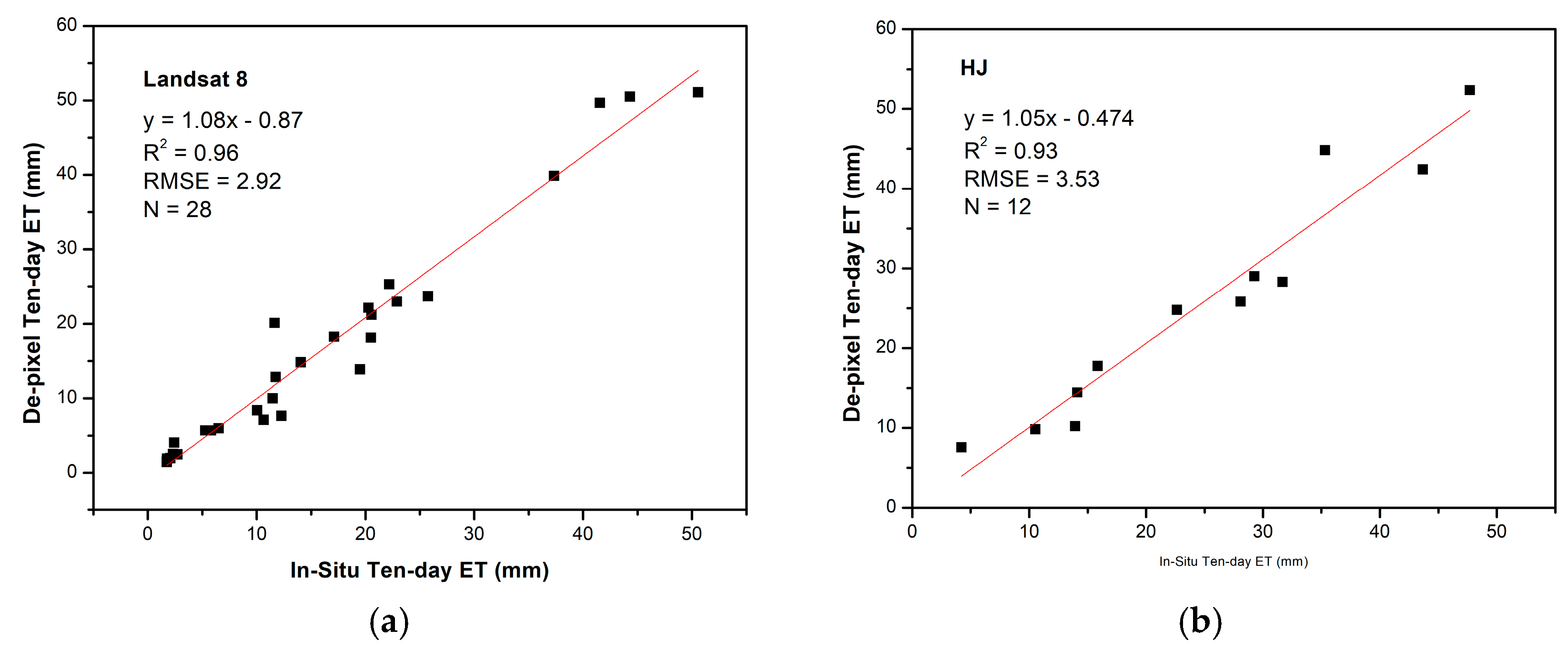
58]. In addition, the existence of this data source with a short repeat interval is one of the reasons why NDVI data are used as the driving factor in the model. To assess the performance of the “de-pixelation” method using NDVI data from different satellites, rather than spectral features,
Figure 8 compares the two datasets obtained using different sensors with the in situ observations.
There is an obvious underestimation of ET in the original MOD16 data and, consequently, in the downscaled results (
Figure 8). As proposed in
Section 4.1, there is a strong correlation between the downscaled results and the original datasets. The mean bias (MB) per month ranges from 41.57 mm at the GT site to 54.62 mm at the DM site, which could lead to serious errors when estimating the actual water consumption. Hence, it is better to choose more accurate coarse ET data or to calibrate the dataset specifically for the research area in order to obtain a better downscaled result.
Based on the comparison of different fine NDVI inputs (
Figure 9), Landsat 8 and HJ, both datasets show good agreement with the ETa from EC. Similar coefficients of determination were obtained (0.96 and 0.93), and the RMSE changes only slightly, from 2.92 to 3.53 per ten-day period. Thus, the HJ satellite may represent a reliable source of NDVI data. This comparison indicates that the NDVI values from different satellites affect the spatial pattern; thus, they influence the ET results. However, this effect has little effect on the ET results, according to the EC validation. This result enables the construction of a stable and continuous downscaled and finer-resolution dataset, based on further research into the normalization of the two sensors.
4.4. Comparison of Different Downscaling Approaches
To evaluate the performance of different models, similar experiments were carried out in the same study area using two other methods, specifically the subtraction method and the LinZi method. The same coarse ETa dataset covering the same time interval was used as the input. In principle, the 30-m Landsat ETa data are needed for both methods as the basic data used to evaluate the correlation between the coarse ETa data at different times. To evaluate the performance of the two approaches on a site-by-site basis, several in situ observations of ET are employed instead of the fine-scale ETa values. The comparison is shown in
Table 7.
Table 7 shows that all three methods display better performance for the relatively homogeneous cropland site (DM) than for the other two sites. In addition, due to the similarities between the subtraction method and the LinZi method, the R
2 results are nearly the same at the three sites. The values of the coefficient of determination obtained at Daman and Guantao using the “de-pixelation” method are slightly higher than those obtained using the other two methods. However, an obviously higher accuracy is observed at the Huazhaizi site. The R
2 value is 0.90 (0.81 for the other two methods), and the MB is 1.55 mm (2.35 for the subtraction method and 5.36 for the LinZi method) at this site. This pattern occurs mainly because the correlation methods concentrate only on the average difference between coarse ETa images, which may filter out some of the extremely high-frequency vegetation signal within semi-arid areas. Therefore, the “de-pixelation” method is more suitable for crop-sparse areas than other downscaling methods.
In regard to the differences in the MB obtained using the three methods, the “de-pixelation” method exhibits the most robust performance among the three methods, with the exception of the LinZi results at Guantao (4.21 mm compared with 4.00 mm). The subtraction method performs well at the Huazhaizi site but poorly at the other two. With several in situ ETa measurements substituting for the fine-scale Landsat ETa input, poorer results are expected for the two correlation methods.
5. Discussion
In this study, a new downscaling approach named “de-pixelation” method, which employs NDVI data and a land cover map with high spatial resolution, is introduced to downscale the ETWatch 1-km ETa data product to a spatial resolution of 30 m. There is a kind of downscaling strategy named “correlation” approaches that are currently widely used, which relies on the relationship between ETa data from two MODIS images (or other high temporal resolution datasets) separated by a given time interval. This relationship is evaluated pixel by pixel or over a small area using either a first-order linear correlation or the difference after subtraction. The linear correlation or the difference is then applied to the fine-scale resolution ET data retrieved from Landsat images. Every Landsat pixel is related to the MODIS pixel it falls inside [
7,
23,
57]. This kind of strategy, including both subtraction and regression (slope-intercept and LinZi) schemes, focuses to a greater degree on the differences among coarse pixels and assumes that all of the finer-scale ET pixels within a given coarse pixel (or within a small area for the slope-intercept method) share the same correlation. These methods do not distinguish between different land cover types; thus, to some extent, they weaken the differences among different land cover types, especially in areas with complex surfaces. Thus, based on the comparison in
Section 4.4, our newly proposed method performs better and more robustly than the other two methods (the two correlation approaches) in crop-sparse areas, such as the HZZ site. Therefore, the new “de-pixelation” method is more suitable for areas with complex land cover distributions.
In this study, monthly Landsat8 NDVI images are used to represent the condition of vegetation at a spatial resolution of 30 m × 30 m. ET products with finer spatial resolutions can be obtained from multi-spectral satellites, such as RapidEye, and additional research is required. Such advances could make it possible to monitor the water use of every land parcel [
59]. In addition, our future work will concentrate on improvements in temporal resolution using the STARFM downscaling method to extend the model to a daily scale by including information from the MODIS 8-day NDVI product. This method could provide additional temporal detail over crop areas [
26,
60].
For the three EC sites within the two study areas examined in this study, representing semi-arid and semi-humid climate types, NDVI saturation did not have an appreciable influence during the growing season because of the limited amount of irrigation water in the Heihe Basin and the two short growing periods in the Haihe Basin. However, further research should be carried out to address the NDVI saturation effect in areas where such conditions occur (especially for crops).
6. Conclusions
Monitoring evapotranspiration using RS-based methods could improve the level of water planning and management through the generation of datasets with both fine temporal and spatial scales. In this paper, a new ET downscaling strategy which combines images from different resolution is proposed. The downscaled results obtained using the “de-pixelation” method show good agreement with the original ETWatch 1-km dataset in terms of temporal changes. Based on the R
2 values between the ETWatch data and the results of the “de-pixelation” method, which range from 0.98 to 0.82, the accuracy of the fine-scale dataset is mainly determined by the corresponding coarse dataset, similar to the findings of other researchers [
26].
Output results also show good agreement with in situ flux observations at three sites, indicating that the new approach represents a reliable substitute for the 30-m ETa dataset in areas with poor coverage by Landsat8 data or other data resources. The new “de-pixelation” method performs well at two relatively homogeneous sites, DM and GT, achieving similar R2 values with respect to the original 1-km ETWatch dataset. However, an obvious improvement occurs at the HZZ site because the original coarse dataset may mix and eliminate some information at the boundaries between vegetation and bare soil.
A comparison between the results obtained using different coarse ETa data sources, MOD16 and ETWatch, is presented based on the analysis of the influence of the accuracy of the coarse data sources. The ETWatch dataset used in this study has been effectively adapted for the two study areas and has been well calibrated; therefore, it performs well. For other data sources, such as the MOD16A2 ET product, improving the adaptability of the original ET dataset to particular regions is expected to increase the accuracy of the downscaled product [
61,
62]. Because the accuracy of the coarse input ET data influences the accuracy of output downscaled dataset, using low-accuracy ET data as an input may cause errors.
Additionally, because of the degree of cloud contamination, two HJ satellite images were substituted for the Landsat8 images in August and September at the two Zhangye sites. A comparison of the results from the two sensors is proposed to provide a validation of this substitute data source. The substitute NDVI data from the HJ satellite does not exert much influence on the final results. This finding makes it possible to generalize the method to areas where Landsat8 images are often affected by clouds through the substitution of other satellite data. Finally, a comparison between “De-pixelation” method and two correlation methods was proposed. The new method performs better at the HZZ site with more complex land cover surrounded. Above all, new downscaling method is suitable for heterogeneous area, to provide robust fine evapotranspiration dataset.


