Article

Three-Dimensional Numerical Study of Free-Flow Sediment Flushing to Increase the Flushing Efficiency: A Case-Study Reservoir in Japan

1
Department of Civil Engineering, Gorgan Branch, Islamic Azad University, Gorgan 49147-39975, Iran
2
Disaster Prevention Research Institute (DPRI), Kyoto University, Uji, Kyoto 611-0011, Japan
3
Hydro-Soft Technology Institute Co., Ltd., Nakanoshima, Osaka 530-6126, Japan
4
Institute for Modelling Hydraulic and Environmental Systems, University of Stuttgart, 70569 Stuttgart, Germany
5
Department of Civil and Environmental Engineering, Norwegian University of Science and Technology, S.P. Andersens vei 5, 7491 Trondheim, Norway
*
Author to whom correspondence should be addressed.
Water 2017, 9(11), 900; https://doi.org/10.3390/w9110900
Submission received: 12 October 2017 / Revised: 10 November 2017 / Accepted: 14 November 2017 / Published: 19 November 2017
(This article belongs to the Special Issue Adaptive Catchment Management and Reservoir Operation)

Abstract

:
The catchment of the Dashidaira reservoir located on the Kurobe River has high sediment yield. Because of the sufficient available amount of water in the catchment during flood events, the free-flow sediment flushing operation with full water-level drawdown is employed every year to preserve the effective storage capacity of the Dashidaira reservoir. This paper focuses first on the numerical simulation of a previously conducted free-flow flushing operation in the Dashidaira reservoir using the available in situ obtained data. Afterwards, to improve the flushing efficiency, the effects of water and discharge manipulation and the construction of an auxiliary channel on the total volume of the flushed sediment were studied. A fully 3D numerical model using the finite volume approach in combination with a wetting/drying algorithm was utilized to reproduce the flow velocity field and simulate the movable bed variations. The outcomes revealed that increasing the average free-flow discharge during the free-flow stage by approximately 56%, in the form of multiple discharge pulses, can enhance the flushing efficiency by up to 13%, and the construction of an auxiliary channel in the wide midstream of the reservoir can locally increase the sediment erosion from this area.

1. Introduction

Dams interrupt the natural continuity of sediment transport through rivers, which results in sediment deposition in the reservoir behind the dam [1]. In a global context, sediment deposition is a challenging issue for the long-term utilization of dam reservoirs [2]. It is estimated that 0.5% of total storage volume of the reservoirs is lost annually in the world because of the sedimentation [3]. The loss of effective reservoir storage volume due to sediment deposition reduces the effective lifespan of dams and decreases reservoir functionality for flood control purposes, hydropower generation, irrigation and water supply, thereby generating a substantial economic loss [1,4,5]. Diverse measures, including sediment dredging, density current venting, bypassing, flushing, sluicing and upstream sediment trapping, have been used to control progressive sedimentation in reservoirs to prolong their life [1,6]. Among these measures, drawdown flushing (i.e., free-flow sediment flushing) plays a major role in reservoir storage capacity restoration and conservation since it is an efficient hydraulic technique for sediment removal [7]. Free-flow sediment flushing involves a complete lowering of the water level by opening low-level outlets to temporarily establish riverine flow (i.e., free flow) through the outlets. The accelerated flow erodes a channel through the deposits and flushes out both fine and coarse sediments [4,5,7]. However, only few experimental studies have focused on flushing channel formation [8], and detailed explanations of flushing channel formation and evolution in prototype reservoirs are scarce [9].
In Japan, the sediment yield coming from the catchments is generally high due to the geologically young mountains, steep slopes, flashy flow regimes, and frequent landslides, especially in the mountainous areas. Thus, a large amount of sediment is transported in Japanese rivers, and the sediment inputs in the reservoirs fed by these rivers are high. Kurobe River, located in the Toyama prefecture, is one of the most important rivers in Japan because of the cascade reservoir system along this river and the considerable amount of electricity generated by water from these reservoirs. Therefore, the reservoir owners are interested in implementing the applicable measures for increasing the sediment removal from these reservoirs especially from the specific areas, which encounters the excess deposition problems.
To optimize the sediment management strategies in reservoirs that feature conditions that change from shallow to deep areas and that also contain sandbars, numerical models that are more complicated than the simple one-dimensional (i.e., 1D) models should be used [10]. Advanced two-dimensional (i.e., 2D) numerical models have been employed to solve practical problems in rivers (e.g., simulation of morphological bed changes in river meanders) [11]. Nevertheless, 2D and quasi three-dimensional (i.e., 3D) numerical models are not able to directly simulate a complex 3D flow field that includes secondary currents. However, these phenomena contribute significantly to the natural sediment transport processes [12]. Thus, the application of 3D numerical models is essential if the velocity variation over the flow depth, i.e., helical flow, plays a major role in sediment transport (e.g., in channel bends). 3D numerical models were used by various researchers for simulating the flow field and sediment transportation in the dam reservoirs [13,14]. As for sediment flushing from reservoirs, a 3D numerical model has been shown to perform better than a 2D one in simulating the bed deformation, notably in channel bends [15]. Recently 3D numerical models were applied to investigate the sediment dynamics inside the reservoirs during a flushing operation at the both lab scale (e.g., [15,16]) and the full scale (e.g., [17,18,19]).
A Computational Fluid Dynamic (CFD) software package called SSIIM (Simulation of Sediment Movements In water Intakes with Multiblock Option) was utilized in this study. The SSIIM program implements a 3D numerical model of the flow field by solving the mass and momentum conservation equation in three dimensions using different turbulence closure approaches [20]. SSIIM was successfully applied to model the 3D flow field under various hydraulic and geometric boundary conditions [21]. SSIIM was also used for coupled computation of the flow and sediment field in physical model and prototype-scale studies by various researchers [22,23,24,25,26,27,28]. Recently, this CFD program was used with enhanced grid generation features to simulate the sedimentation and flushing channel evolution in reservoirs [19,29,30]. Nevertheless, it should be noted that simulation of a sediment-flushing event in a steep full-scale reservoir, such as the Dashidaira reservoir, is complex owing to the rapid variation of hydraulic boundary conditions and riverbed materials even in short distances. In addition, numerical studies focusing on potential measures for increasing the sediment flushing efficiency in a full-scale reservoir are scarce.
In the present study, the SSIIM model was employed to simulate the 2012 free-flow sediment flushing operation in the Dashidaira reservoir using the field-measured data. To do this, the sensitivity analysis of computed Total Volume of Flushed Sediments (i.e., TVFS) as a result of changes in the selected empirical parameters together with assessment of morphological bed changes was performed and subsequently model was calibrated. Because of the interest to increase the Flushing Efficiency (i.e., FE), when it is defined as the ratio of the flushed sediment volume to the used water volume, various scenarios, such as using additional artificial discharge during the free-flow state, increasing the water-level drawdown speed, and the construction of an auxiliary longitudinal channel, were numerically modeled to investigate how they affect the morphological bed changes in specific zones of the reservoir and whether they increase the Flushing Efficiency. To provide a more detailed and quantitative insight on morphological bed changes, the Bed Changes Index (i.e., BCI) is introduced and subsequently calculated bed changes were compared for each scenario with a reference case (e.g., calibrated case) to figure out the performance of each scenario. Moreover, the optimum relationship between the flushing efficiency and the amount of water used for flushing was established under the mentioned scenario conditions.

2. Study Case Description

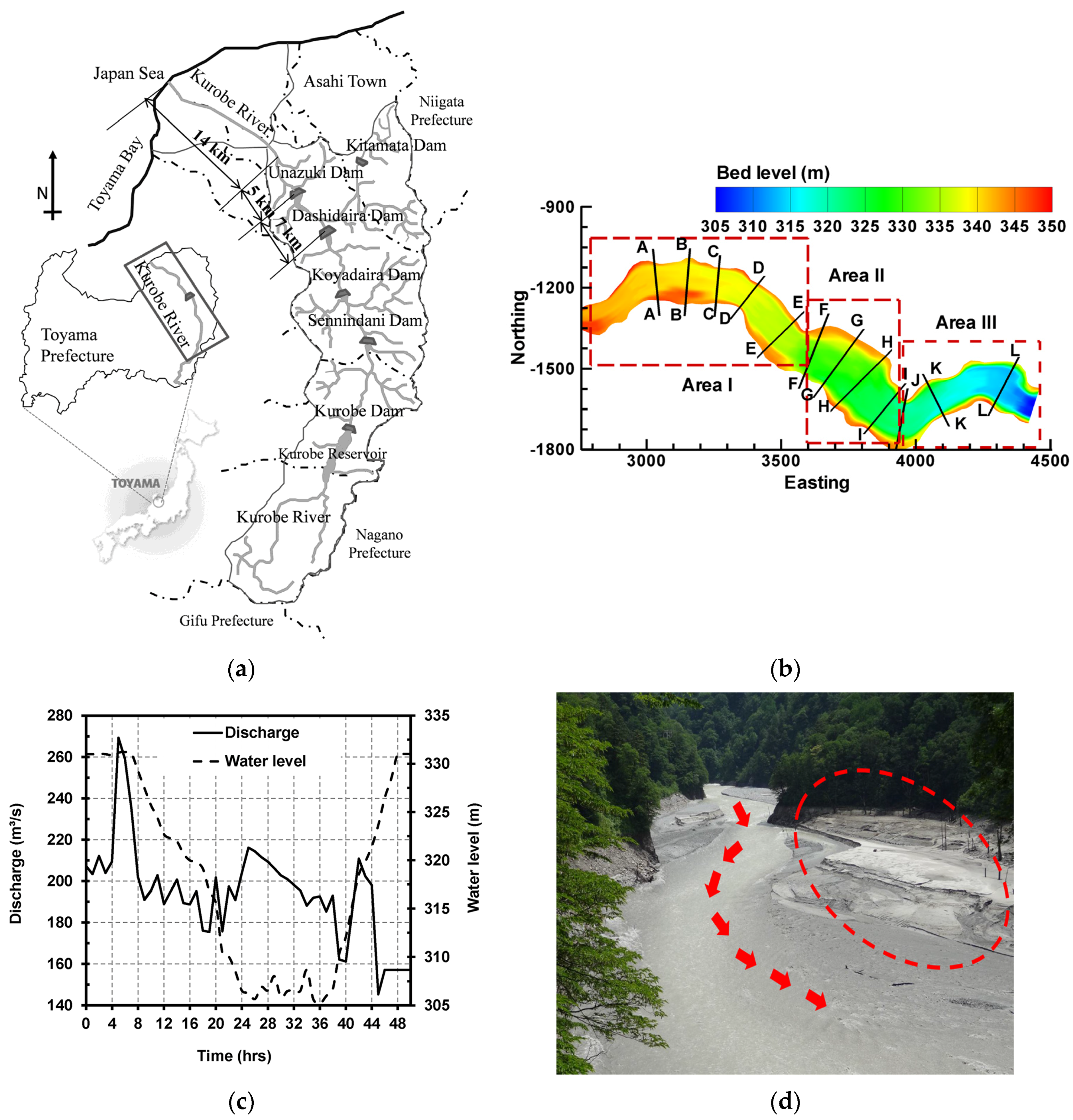
2.1. Site Background

The Kurobe River originates from Washiba Mountain with an elevation of 3000 m, located in the northern Japanese Alps, and flows into Toyama bay in the Japan Sea (Figure 1a) [31]. The catchment area of the river is 682 km2, and the length of the river is 85 km. The bed slope is steep and varies between 1% and 20%. In the catchment area of the Kurobe River, the average rainfall and total sediment yield are 4000 mm and 1.4 × 10⁶ m3/year, respectively, which are both among the highest in Japan [32]. Dashidaira dam, with a height of 76.7 m, was constructed in 1985 by Kansai Electric Power Company in the Kurobe River and has a power of 124 MW. The average bed slope of the reservoir is about 2.2% and also the gross and effective storage capacities are 9.01 and 1.66 million m3, respectively [7,32]. The mean annual sediment load and the ratio of the total storage to the mean annual runoff in the Dashidaira reservoir are 0.62 × 10⁶ m3 and 0.00674, respectively [33]. The Dashidaira dam is one of the first dams in Japan constructed with sediment-flushing facilities. The first flushing operation in the Dashidaira reservoir was performed 6 years after the dam construction in 1991. Subsequently, the accumulated distorted sediments within 6 years were diffused to the downstream and estuary zone with many negative environmental implications. After that, the flushing operation is performed every year during the first major flood event in the rainy season to reduce negative environmental impacts on the downstream areas of the dam since aquatic animals have been adapted to the perturbation caused by floods. A flood not only provides enough energy to transport the flood-born sediments through the reservoir, but also scour the previously deposited sediments from the reservoir.

2.2. Field Data Organization

The bathymetric survey for measuring the bed levels is performed regularly by the reservoir owners before and after the annual flushing operation in the Dashidaira reservoir. The measured bed levels before the flushing operation in June 2012 and the locations of cross-sections A-A to L-L, which were used for further assessment of bed variations caused by the flushing, are shown in Figure 1b. The approximately 2-km length of the reservoir has been divided into three areas, namely, areas I, II and III, to analyze the study outcomes based on the generally similar types of bed materials in each area. In area I, the bed material is coarse (e.g., gravel), while in downstream half of area II and the area III, the bed material transitions to finer sediments (e.g., fine sand and even mud). Besides, temporal variation of the water level and discharge magnitudes are recorded at the dam site during the flushing. The inflow discharge and water level fluctuations during the 2012 flushing operation, in which the major sediment inflow was a wash load (i.e., transported without deposition in the reservoir), are illustrated in Figure 1c. After the start of the operation, the preliminary drawdown occurred from 8 to 24 h, and the free-flow state occurred from 24 to 38 h. The water level drawdown from the beginning of the operation to the free-flow state was approximately 25 m. Furthermore, based on the available onsite samples, seven sediment sizes ranging between 316 and 0.37 mm were considered to be representative grain sizes for the bed of the reservoir. Table 1 shows the average sediment size distribution in different cross-sections prior to the flushing operation. The large sediment sizes in cross-section L-L despite the size reduction in sections immediately upstream can be attributed to the last flushing operation process, in which closing the bottom outlets during the water level recovery stage causes the transported large sediments to deposit nearby the dam. During the 2012 flushing operation of the Dashidaira reservoir, the total volume of the eroded sediment from the reservoir was equal to 408,700 m3.
The thalweg of the river channel exists close to the right bank of the wide middle area (i.e., area II) and subsequently fine sediments deposited along the left bank, indicated with an ellipse dashed line in Figure 1d, were not removed effectively during the flushing operation. Therefore, fine sediments have been accumulated and consolidated that may contain the degraded organic matters. The area highlighted by the ellipse dashed line is hereafter called the dead zone. Dam owners are interested in removing the accumulated sediments from this zone by annual flushing operation to prevent the formation of consolidated and distorted fine sediments and also to keep the effective storage capacity as much as possible.

3. Numerical Model

3.1. Flow Field Modeling

The fully 3D numerical model SSIIM solves the continuity equation together with Reynolds-averaged Navier-Stokes equations in three dimensions and within non-orthogonal coordinates to compute the water motion for turbulent flow [20].
The finite-volume approach is applied as a discretization method to transform the partial differential equations into algebraic equations. The convection term in the Navier-Stokes equation is solved using the second-order upwind scheme [15,20]. The Reynolds stress term is modeled using the standard k-ε turbulence model with constant empirical values [34].
The unknown pressure field in the Reynolds-averaged Navier-Stokes equations is calculated by employing the semi-implicit method for pressure-linked equations [35]. An implicit free-water surface algorithm was used in the computations and was based on the pressure gradient between a cell and the neighbor cells. Then, the free-water surface is computed using the local elevation difference between a cell and the neighboring cells [19].
p x i = ρ g z x i
where p is the pressure, xi is the special geometrical scale, ρ is the water density, g is the acceleration due to gravity and z is the water-level elevation.
Because the water level in all cells is unknown, an iterative method was used. Additionally, because a number of neighbor cells were used to compute the water elevation differences for each cell, different values appeared for the water elevation difference depending on the number of neighboring cells used in the computation. Therefore, a weighted average of these values was applied. The weighted average coefficient for each neighboring cell (ai) is a function of the Froude number, the flow direction and the location of neighboring cells:
a i = { m i n ( 2 F r ; 1.0 )    f o r   w > 0.1   a n d   F r < 2.0 w 2 ( F r 1.0 )       f o r   w < 0.5   a n d   F r > 2.0 0.0
with:
w = r × u | r | × | u |
where Fr is the Froude number, w is the dot product of r and u , is r the direction vector pointing from the center of a cell to the center of the neighbor cell aimed to take into account the upstream/downstream effect and u is the velocity vector of the cell. This coefficient is then used for discretizing the following equation [19]:
i = 1 8 a i z p = i = 1 8 a i ( z i + 1 ρ g ( p p p i ) )
where zp is the water level elevation in the cell, zi is the water level elevation in the ith neighbor cell, pp is the pressure in the cell and pi is the pressure in the ith neighbor cell.
This implicit and iterative approach is a robust and stable method that can also be used in connection with estimates of the sediment transport and morphological bed changes under unsteady flow conditions. The use of an implicit discretization scheme allows large time-step sizes to be employed in the model [23].
In the SSIIM model, the grid is non-orthogonal, unstructured and adaptive, and it moves vertically with changes in the bed and free-water surface elevation. During the computations, only the water body is modeled. The water surface is recomputed after each time step, and the employed wetting/drying algorithm enables the model to have a varying number of grid cells (e.g., in the vertical and lateral directions) with respect to the water depth in the computational domain using Equation (5) [36]. The wetting/drying algorithm causes the cells to dry up and disappear from the computational domain if the water depth is smaller than a user-defined lower boundary. If the water depth becomes greater than the lower boundary in the dry area, this algorithm regenerates a cell. This approach makes it possible to have a dynamic grid that can move in the lateral direction, allowing changes in the bed and water level to be accurately modeled.
n = n m a x ( d e p t h d e p t h m a x ) p
where n is the number of grid cells in the vertical direction, nmax is the maximum number of grid cells in the vertical direction, and p is a user-defined parameter for the number of grid cells.
The Dirichlet boundary condition (logarithmic velocity distribution) was used for the water inflow, whereas the zero-gradient boundary condition was specified for the water outflow and the sediment concentration calculation. For the boundary condition at the bed and walls, where there is no water flux, the empirical wall law introduced by Schlichting (1979) was utilized [20,37]. Also, bed roughness in the form of dunes and ripples is taken into account using an empirical formula introduced by Van Rijn, which employs the characteristics of sediment size distribution and bed form height within the computational domain [20,38].

3.2. Sediment Transport Modeling

The sediment transport computation for simulating the morphological changes is divided into suspended sediment and bed load transport. The suspended sediment transport is calculated by solving the transient convection-diffusion equation.
c t + U j c x j + w c z = x j ( Γ T c x j )
where Uj is the water velocity, w is the fall velocity of the sediments, c is the sediment concentration over time t and spatial geometries (i.e., x and z), and ΓT is the turbulent diffusivity. To compute the equilibrium suspended sediment concentration, used as the boundary condition in the cells close to the bed, an empirical formula developed by Van Rijn is used [39]:
C b e d = 0.015 d i a [ τ τ c , i τ c , i ] 1.5 ( d i [ ( ρ s ρ w ) g ρ w ν 2 ] 1 / 3 ) 0.3
where a is a reference level set equal to the roughness height, di is the diameter of the i-th fraction, ν is the kinematic viscosity, τ is the shear stress, τc,i is the critical shear stress for di, which was calculated from the Shield’s curve, and ρw and ρs are the density of the water and sediment, respectively.
In the SSIIM model, the bed load can be simulated using the Van Rijn formula or alternatively by the Meyer-Peter-Müller (MPM) formula [40,41]. The MPM formula is appropriate for steep rivers, which mainly transport coarse sediments close to the bed:
q b , i = 1 g [ ρ w g r I 0.047 g ( ρ s ρ w ) d 50 0.25 ρ w 1 3 ( ρ s ρ w ρ s ) 2 3 ] 3 2
where qb,i is the sediment transport rate for the i -th fraction of the bed load per unit width, d50 is the characteristic sediment size (median sediment size), r is the hydraulic radius, and I is the slope of the energy line. The Van Rijn formula has been used to simulate a wide variety of sediment transport issues in both physical model and prototype scales:
q b , i d i 1.5 ( ρ s ρ w ) g ρ w = 0.053 [ τ τ c , i τ c , i ] 1.5 d i 0.3 [ ( ( ρ s ρ w ) g ρ w ν 2 ) ] 0.1
The model accounts for side slope effects by utilizing a reduction function of the critical shear stress for incipient motion by introducing the formula of Brooks together with a sand slide algorithm [20,42]. The sand slide algorithm corrects the bed slope if it exceeds a defined critical angle of repose of the sediments during excessive erosion and thereby accounts for side bank erosion. In fact, the implemented sand slide algorithm acts as a limiter when erosion continues and the bed slope increases [26].

4. Numerical Simulations

4.1. Model Setup and Calibration

The computational grid was constructed based on the bathymetric surveys before the flushing (Figure 1b). The mesh cell sizes in the streamwise and transversal directions were 10–20 m and 5–10 m, respectively. The bed material density was assumed to be 2650 kg/m3. The water levels and inflow discharge fluctuations, which were employed as the hydrodynamic boundary conditions in the simulations, are shown in Figure 1c. In addition, a non-uniform bed material size distribution with spatially varying fractions was introduced to the model by using the seven representative sediment sizes shown in Table 1. More specifically, the computational domain was divided into a number of small segments, and each segment had its own non-uniform grain size distribution. Because the wash load, by its definition, is transported without deposition through the reservoir, its effect on the simulation of the flushing process was neglected in the computations.
For calibration purposes, a reference case was first established, assuming general values for the empirical parameters in the SSIIM model. Due to the good performance of the MPM bed load sediment transport formula for flushing simulations of Alpine reservoirs revealed by Haun et al. with conditions almost similar to those of the Dashidaira reservoir (e.g., steep slopes and a wide variety of sediment size distributions) [29], this sediment transport formula was selected for the reference case and subsequently for the sensitivity analysis and model calibration. Then, the sensitivity of the computed TVFS to changes in the empirical parameters was investigated. The computed TVFS was compared with the measured TVFS (i.e., 408.7 × 10³ m3), and if it was larger than 75% compared to the measured one, it was considered a model case for further assessment. Then, the final simulated bed topography pattern was compared, both qualitatively and quantitatively, with the measurements. A qualitative assessment was performed to check whether the erosion in area I, where the coarser sediments exist, could be captured, and a quantitative assessment was conducted to measure the deviation of the simulated bed levels from the measured ones. Therefore, Mean Absolute Error (MAE) of the simulated bed levels after the flushing operation was calculated. Table 2 summarizes the results of the TVFS sensitivity analysis for the major selected empirical parameters. Also, variations in the MAE of the simulated bed levels for each case have been calculated. The TVFS increased with increasing the active layer thickness and water content but decreased with increasing the critical angle of repose. When a larger amount of bed materials can be eroded during one time step (i.e., a thicker active layer), a higher volume of erosion from the deposits is expected. A higher water content in the sediment deposits (e.g., 50%), which decreases the submerged density of the bed material, is assumed to lead to greater sediment entrainment. A higher critical angle of repose retains a steeper side bank of the flushing channel after each time step, resulting in further deepening of the channel, which is not an efficient approach for increasing the TVFS in the numerical model. In contrast, the lateral development of the flushing channel (i.e., channel widening), which is favorable for increasing the TVFS, can be achieved using a lower critical angle of repose. The roughness, active layer thickness, water content of the bed material, and critical angle of repose were after the calibration set to 0.5 m, 1 m, 40% and 32 degrees, respectively, because the application of these values can result in a reasonable TVFS and accuracy (i.e., 313.0 × 10³ m3, and 1.8 m) and can also satisfy the mentioned qualitative criteria.

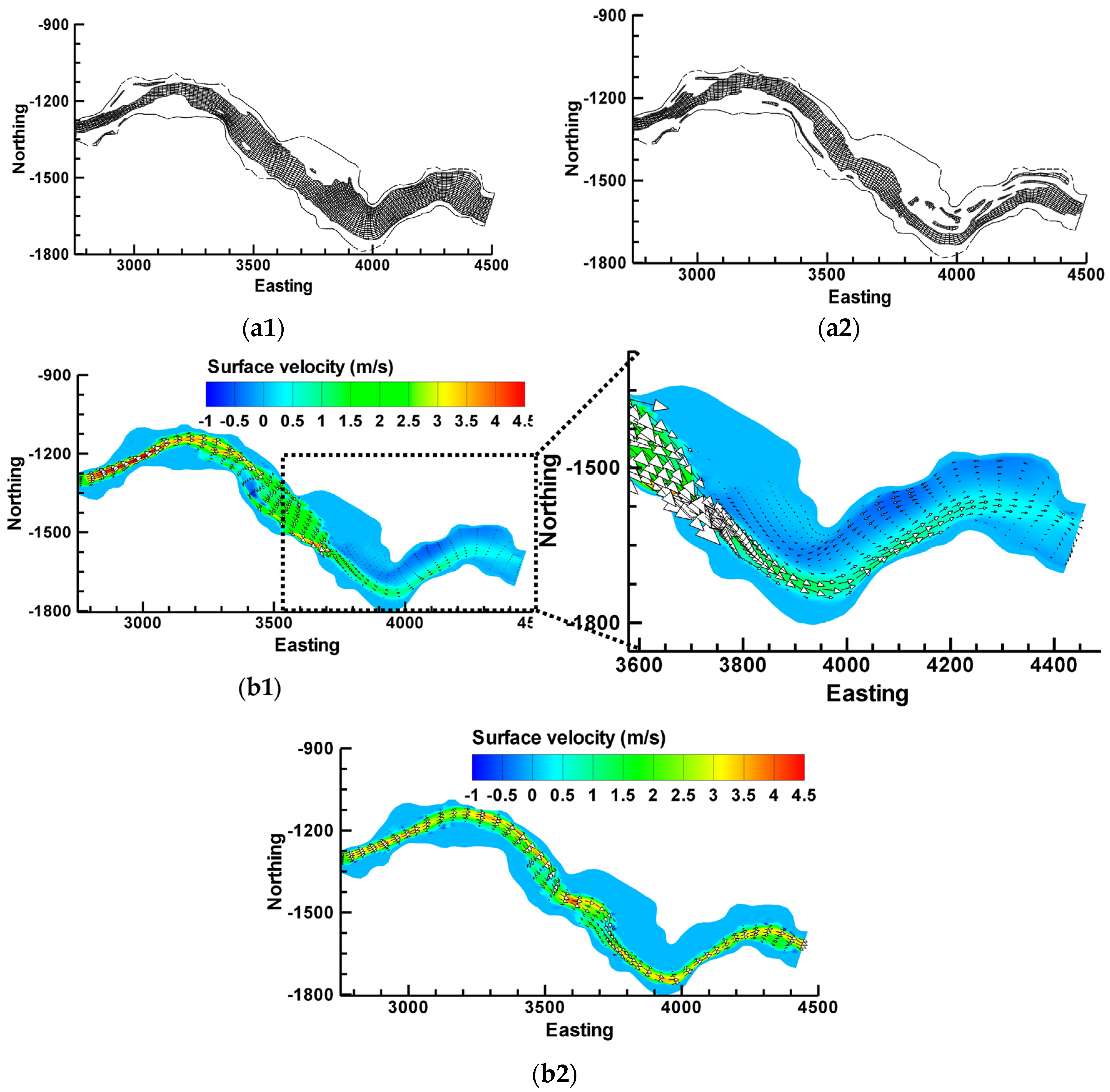
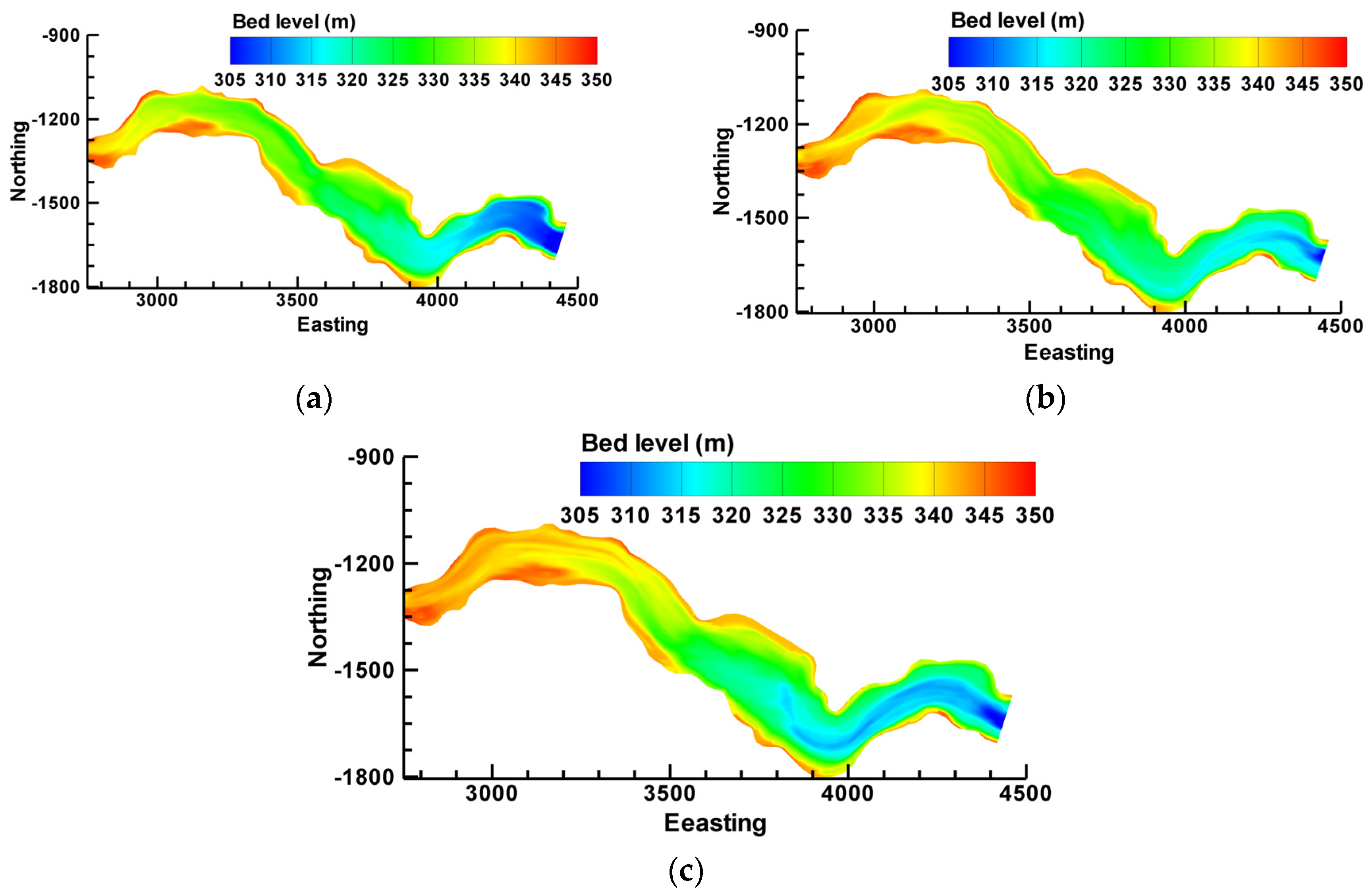
4.2. Evaluation of the Flow Field and Morphological Bed Changes in the Reservoir

Figure 2 shows the computational grid adjustment at the beginning (i.e., t = 10 h; Figure 2(a1)) and during the free-flow conditions with a low water head in the reservoir (i.e., t = 32 h; Figure 2(a2)), and corresponding surface water velocity field (i.e., Figure 2(b1,b2)). The cells with a smaller water head than a specified value were removed from the computational domain due to the employed wetting/drying algorithm. The grid adjustment also reveals that the flow was deflected to the right-hand side of area II during the free-flow conditions; consequently, the flushing channel location was close to the right bank. Figure 2(b1) shows that a complex flow field with a strong reverse flow pattern and water stagnant zone develops in the lower half of the reservoir. This can be attributed to the complex geometry of the computational domain, the variation in flow depths from shallow conditions in the upstream areas to deep conditions in the downstream areas, and the existing bed roughness of the computational domain. In addition, Figure 2(b2) shows the water flow concentration in the flushing channel when the water level is lowest in the reservoir. During the free-flow condition, as shown in Figure 2(b2), the velocities rise to approximately 4.5 m/s, and supercritical flows are likely to develop in several zones of the flushing channel. However, the 3D numerical model can capture the complex characteristics of the flow field in channel bends (i.e., erosion along the outside of the bend and deposition along the inside) and reproduced the non-symmetrical velocity profile over the width and the tilting the lateral water surface at the apex of the channel bend [43]. As can be observed from Figure 2(b1,b2), the wet area of the computational domain contains the water body and the corresponding surface velocity vectors so that it is distinguished from the dry area without surface velocity vectors. An approximately 2-m-thick deposit along the left bank of the dead zone, shown in Figure 1d, can be attributed to the reverse flows that developed beside the bank of the reservoir during the drawdown stage as shown in Figure 2(b1) and that transported suspended fine materials into the stagnant water zone.
Figure 3a illustrates the measured bed topography after the 2012 flushing operation in comparison with the simulated final bed topography after the flushing operation using the MPM and Van Rijn formulas (Figure 3b,c, respectively). To provide more quantitative insights into the simulated final bed topography after the flushing operation the BCI is defined as follows:
BCI = i = 1 n ( z i _ m s z i _ r e f e r e n c e ) n
where zi_ms is the measured or simulated bed level after the flushing operation at each grid node and zi_reference is the measured or simulated reference bed level at the corresponding node, which is used for comparison purposes to provide information about erosion or deposition over a specific zone of the computational grid. Furthermore, n is the number of grid nodes considered for comparison purposes. Positive and negative values of BCI represent depositional and erosional conditions, respectively. In other words, BCI reveals the average change in the bed level of each target zone and readily indicates the dominant morphological process (i.e., erosion or deposition) in the zone compared to the reference case.
BCI parameter was extracted in different areas of the reservoir using the measured bed levels after flushing and for calculations based on the MPM and Van Rijn bed load sediment transport formula when the measured bed levels before flushing (Figure 1b) are considered as reference case. In the upstream area I, the measurements reveal an average erosion value of 2.03 and simulated bed levels via MPM and Van Rijn formula in the calibrated case show average erosion value of 1.61 and 0.15 m, respectively. In this area, the performance of the MPM formula was better than Van Rijn formula in prediction of the morphological bed changes. In the wider midstream segment (i.e., area II), the measurements using the BCI parameter reveal an average erosion value of 0.67 m whereas simulated bed levels via MPM and Van Rijn formula show average erosion value of 1.59 and 3.11 m, respectively. The predicted morphological bed changes in this area obtained using the MPM formula were less overestimated than those obtained using the Van Rijn formula. In the area close to the dam (i.e., area III), the results of the simulations showed a narrower flushing channel compared to the measurements, regardless of the sediment transport formula used [43].

5. Discussion

5.1. Hydrodynamic Scenarios and Their Impacts on the Bed Morphology and Flushing Efficiency

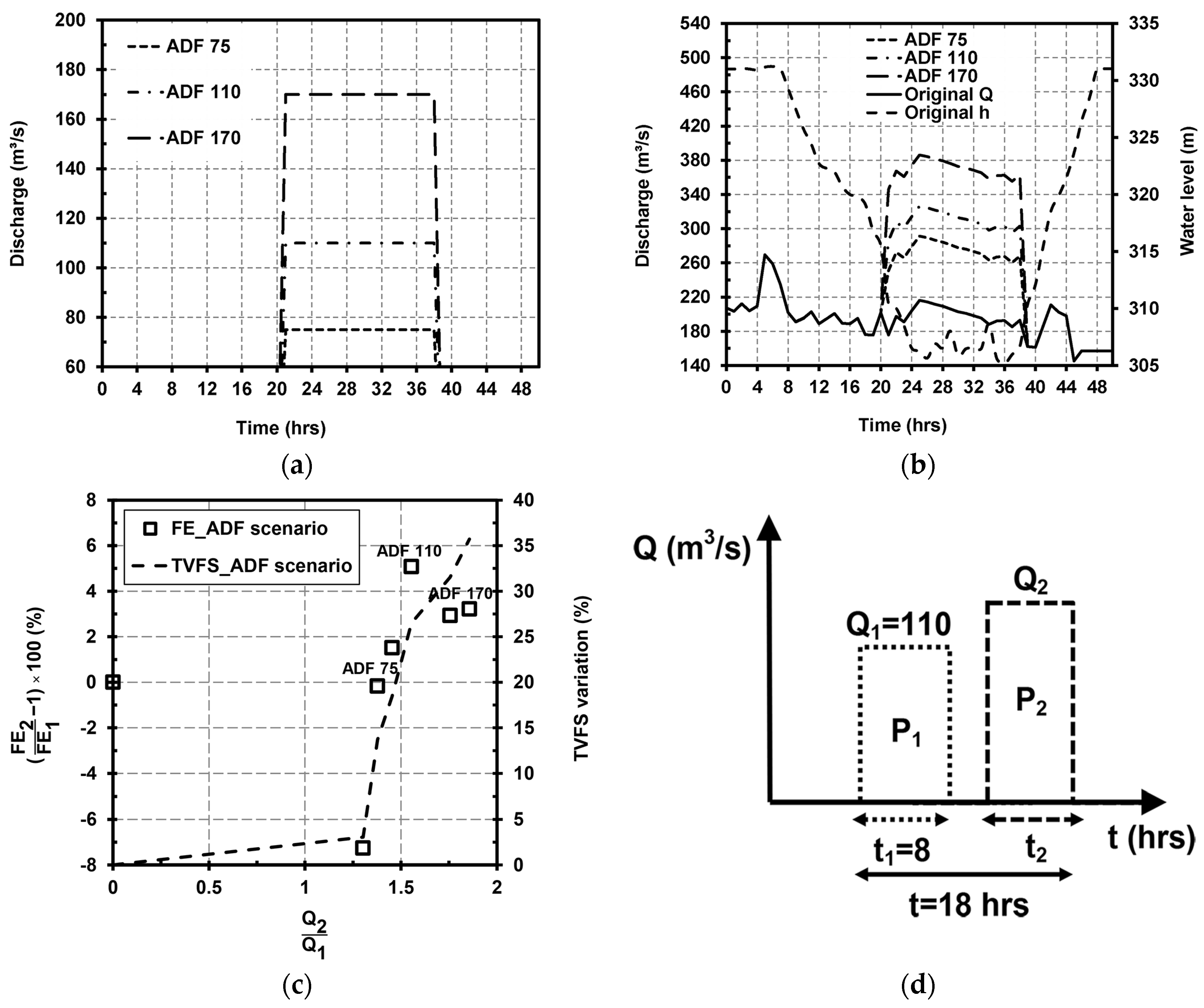
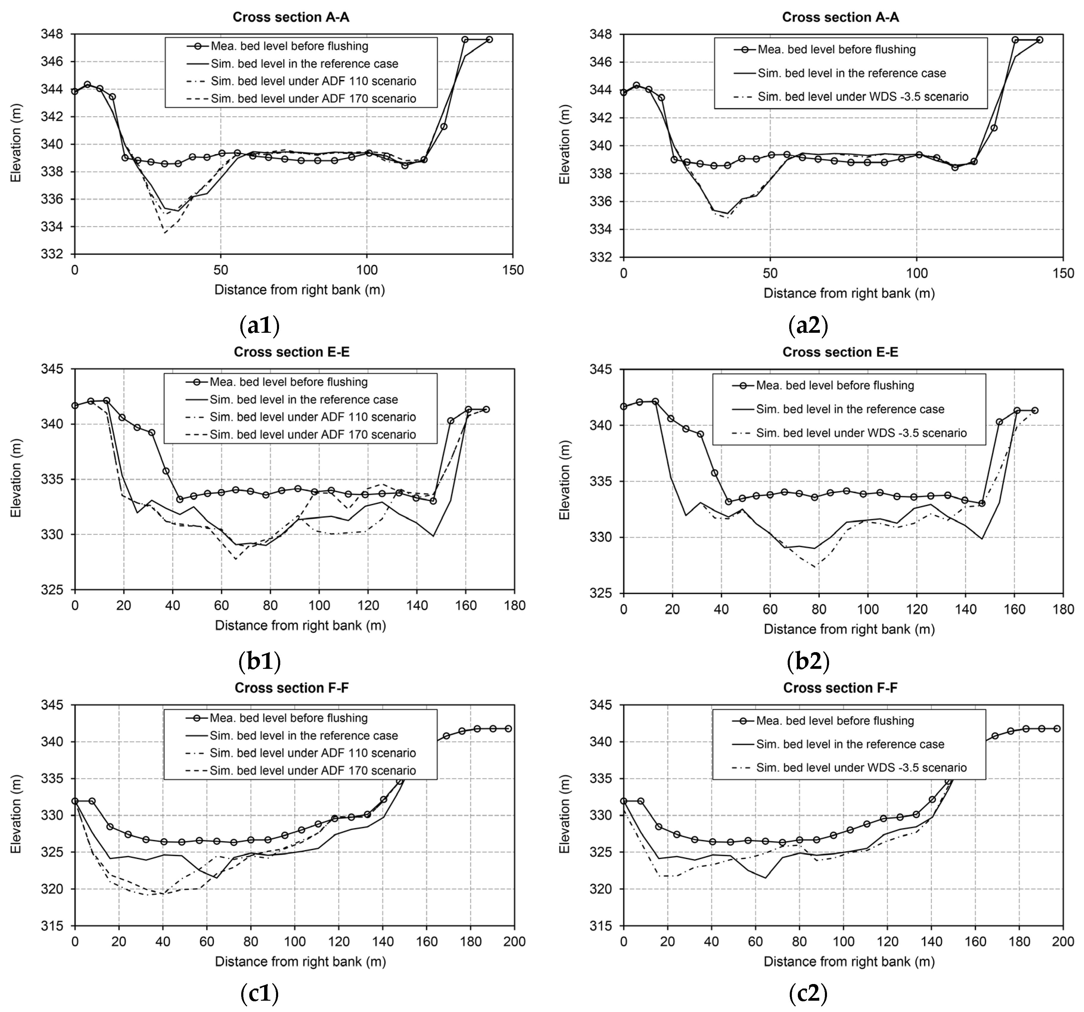
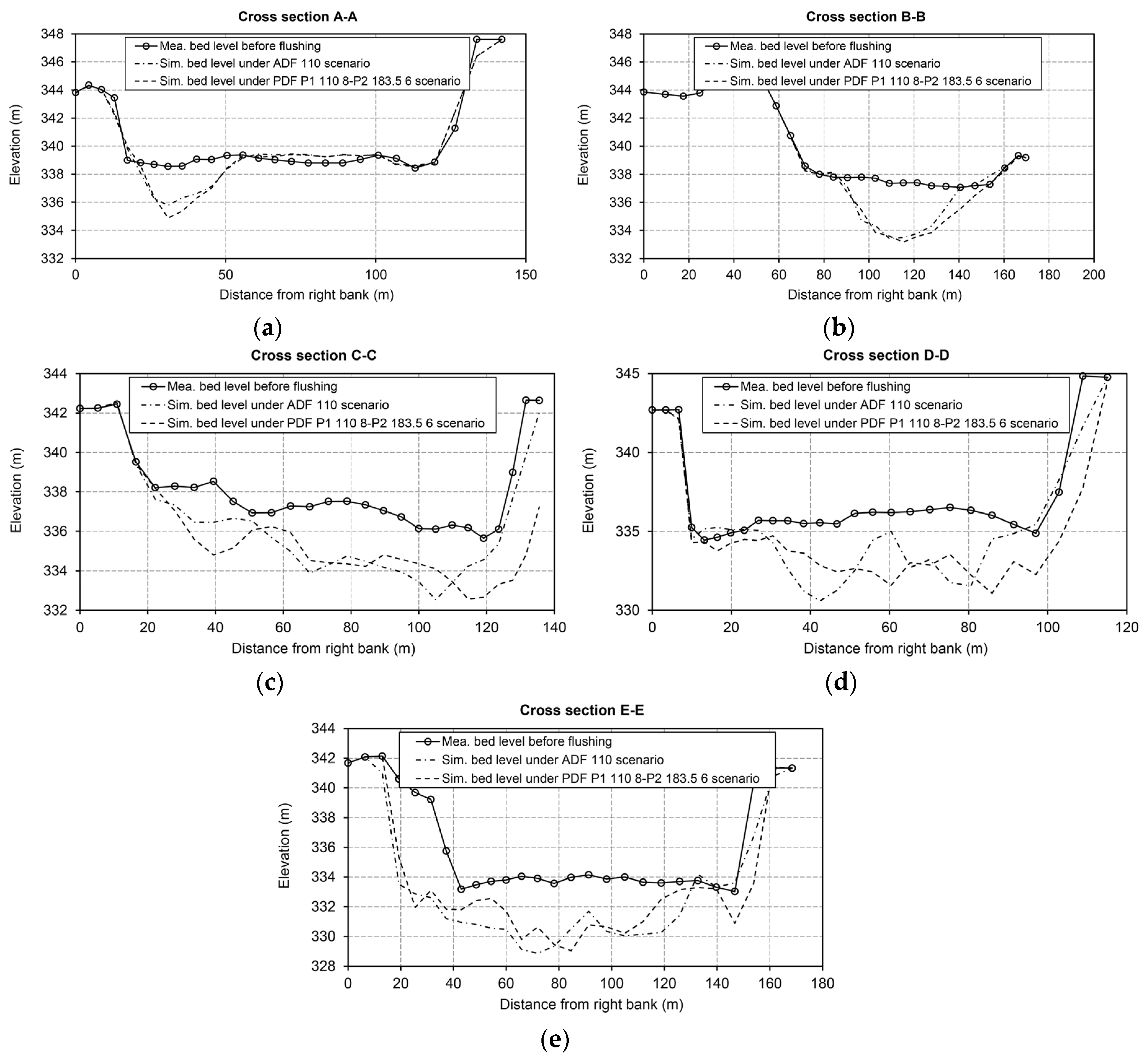
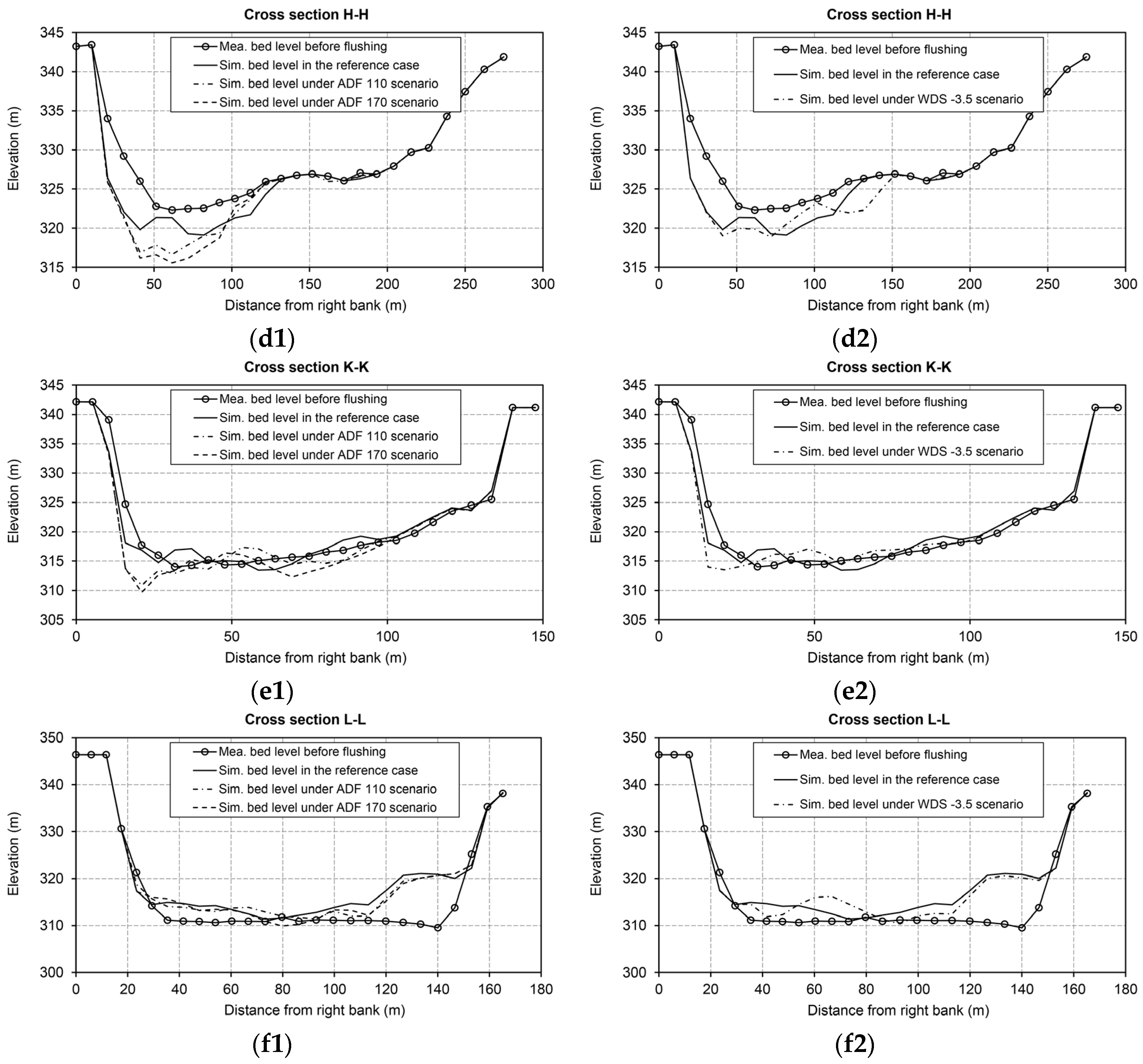
5.1.1. Discharge Scenarios

One of the feasible scenarios in the Dashidaira reservoir is the introduction of an Additional inflow Discharge during the Free-flow stage of the flushing operation (i.e., the ADF scenario). The additional discharge could be supplied from reservoirs located upstream of the Dashidaira reservoir. This additional inflow could enhance sediment entrainment by increasing the average flow velocity and bed shear stress in the Dashidaira reservoir. The ADF scenario is currently applicable, and preliminary tests for this scenario are being implemented in the Dashidaira reservoir.
Figure 4a shows the additional inflow that could be supplied in different ADF scenarios, and Figure 4b shows the discharge rates and original water level (i.e., Q and h, respectively) together with modified discharge rates under different ADF scenarios in the Dashidaira reservoir. Under the different ADF scenarios, the original boundary conditions of the water level (i.e., recorded during the 2012 flushing operation) have been retained, but the original boundary conditions of the discharge during the free-flow stage of the 2012 flushing operation change depending on which ADF scenario is used. For instance, ADF 110 indicates that 110 m3/s of additional inflow discharge has been added to the original discharges during the free-flow stage of the 2012 flushing operation. With an original TVFS value equals to 313.0 × 10³ m3 in the reference case (i.e., resulting bed topography after simulation of 2012 flushing), the TVFS increased to 356.0 × 10³ in the ADF 75 scenario, 396.1 × 10³ in the ADF 110 scenario, and 425.0 × 10³ m3 in the ADF 170 scenario. The effects of introducing constant additional discharges under various ADF scenarios on the FE and the TVFS are illustrated in Figure 4c. The horizontal axis shows the ratio of average discharge during the free-flow stage using different ADF scenarios (i.e., Q2) to the average discharge during the free-flow stage when no additional discharge is introduced in the reference case (i.e., Q1). FE2 and FE1 are the flushing efficiencies when an ADF scenario is employed and when no additional discharge is employed in the reference case, respectively. The TVFS increases when the discharge increases during the free-flow stage. The FE values reached approximately −6.5% when the ADF 60 scenario was used. In this case, the increase in the flushed sediment volume was smaller than the increase in the used water volume according to the FE definition. Under the ADF 75, 90, and 110 scenarios, both the FE and TVFS increased with increasing average discharge during the free-flow stage. Then, the FE variation trended downward until a stable level was reached for the ADF 150 and ADF 170 scenarios. In contrast, the TVFS continued to increase. Under the given conditions, increasing the discharge magnitude during the free-flow condition can increase the TVFS, but this increase is not proportional to the discharge increase that causes the decrease in the FE for some cases. According to the diagram shown in Figure 4c, when the average discharge during the free-flow stage increased by approximately 56% under the ADF 110 scenario, (i.e., Q2/Q1 = 1.56), the FE increased approximately by 5%. Under these conditions, the total used water volume for the flushing operation increased by approximately 21%. In Table 3 the average bed level changes compared to the reference case using the BCI parameter in the upstream, midstream and downstream areas have been revealed for the ADF 75, ADF 110, and ADF 170 scenarios. As shown in Figure 4c and Table 3, introducing additional discharge increases the erosion in all areas by between 3% and 36% depending on the additional discharge, but the effect in the areas close to the dam (i.e., areas II and III) is more pronounced. Instead of adding a constant discharge to the original discharge values during the free-flow condition in the reference case, another scenario (i.e., the PDF scenario) using the same additional water volume over a shorter duration and in the form of discharge pulses was tested. The PDF scenario was introduced to determine whether changing the characteristics of the additional inflowing water (e.g., the discharge intensity) markedly affects the quantity of flushed sediments and the bed changes in specific zones of the reservoir. The concept of the PDF scenario has been illustrated schematically in Figure 4d. It should be noted that before the flushing operation, area III was mainly covered with fine materials. During the simulation of the flushing operation, eroded coarser materials from area I were deposited in the lower parts of area III due to the reduced bed shear stress. Thus, introducing an additional discharge during the free-flow condition can contribute to flushing the deposited sediments out of this area.
Because the best FE correlation was found for the ADF 110 scenario as shown in Figure 4c, the total volume of the additional water used during the 18 h of the free-flow stage was calculated, and this additional water volume was introduced into the model in the form of two discharge pulses, the first one in the first half of the free-flow stage (i.e., P1) and the second one (i.e., P2) in the second half. More specifically, in the PDF scenario, a constant 110 m3/s discharge pulse within 8 h in the first half of the free-flow flushing (i.e., P1 110 8) and a second discharge pulse with variable magnitude and duration in the second half (i.e., P2 Q2 t2) were introduced for further assessments.
In Figure 5, the bed changes with and without the introduction of the additional discharge (i.e., the reference case, ADF 110, and ADF 170) have been plotted at the cross-sections A-A, E-E, F-F, H-H, K-K, and L-L. As can be observed from Figure 5(f1,f2), instead of erosion, deposition occurs in cross section L-L. At the end of free-flow stage during the flushing process, bottom outlets are closed and water level starts to increase beside the dam while it is still low in the upstream portions of the reservoir and free-flow condition exists. In such a condition, the induced bed shear stress is reduced noticeably in areas close to the dam. Therefore, the eroded large size sediments are still transported towards downstream but they are deposited close to the dam without chance to flush. Table 3 reveals that the introduction of an additional discharge during the free-flow condition, in ADF scenarios, has a marginal effect on the erosion of coarser sediments in area I. This pattern can be attributed to the major role of the water-level drawdown stage in the initial development and evolution of the flushing channel, as revealed by experimental and numerical model studies by Esmaeili et al. and Kantoush and Schleiss [30,44]. Notably, from the reservoir entrance up to the cross-section A-A, the BCI values showed 0.04, 0.06, and 0.10 m of erosion under ADF 75, 110, and 170 scenarios compared to the simulated bed levels after 2012 flushing operation. Because the BCI values indicate overall deposition in area I, the eroded coarser bed materials from the area upstream of section A-A are likely deposited again after passing the cross-section A-A as a result of the increasing flow depth and the consequent velocity reduction. This process prevents the smaller grain size bed materials underneath from being eroded. However, if the deposition of coarser materials occurs in the main flushing channel, the erosion will increase, even with a smaller additional discharge (e.g., in the ADF 75 scenario) due to an increase in the bed shear stresses in the channel. In addition, the inflowing discharge during the free-flow condition is concentrated in the central flushing channel, which mainly contributes to a slow widening and deepening of the existing channel. This widening and deepening process is more effective in areas covered by finer sediments (e.g., areas II and III). Thus, use of the 170 m3/s of additional inflow during the free-flow stage may result in a further increase in the flushing channel width and depth in the lower part of area II and throughout area III.
Also, the resulting BCI parameter for the PDF scenario has been shown in Table 3. Using the PDF scenario not only enhanced the TVFS by increasing the erosion from areas II and III but also increased the erosion of coarser material from area I when the second discharge pulse was sufficiently high (i.e., PDF P1 110 8-P2 183.5 6). These increases can be attributed to the transport of already eroded coarser materials from area I to farther downstream areas due to a higher induced bed shear stress. Increasing the TVFS under the PDF scenarios, can increase the FE about 13% compared to the reference case. Nevertheless, due to the further deposition of sediments eroded from the head of the reservoir in the dam vicinity, the bed level changes appear to be marginal compared to the ADF 110 scenario when the second discharge pulse is high. Figure 6 shows the bed changes in different cross-sections in area I under the PDF P1 110 8-P2 183.5 6 scenario compared to the bed changes using the ADF 110 scenario to quantitatively show the advantageous performance of the PDF scenario in eroding the coarser bed materials in area I. However, the use of ADF or PDF scenario does not affect the main flushing channel location close to the right bank in area II. Consequently, the deposited bed materials close to the left bank in area II (i.e., the dead zone) still cannot be effectively removed.

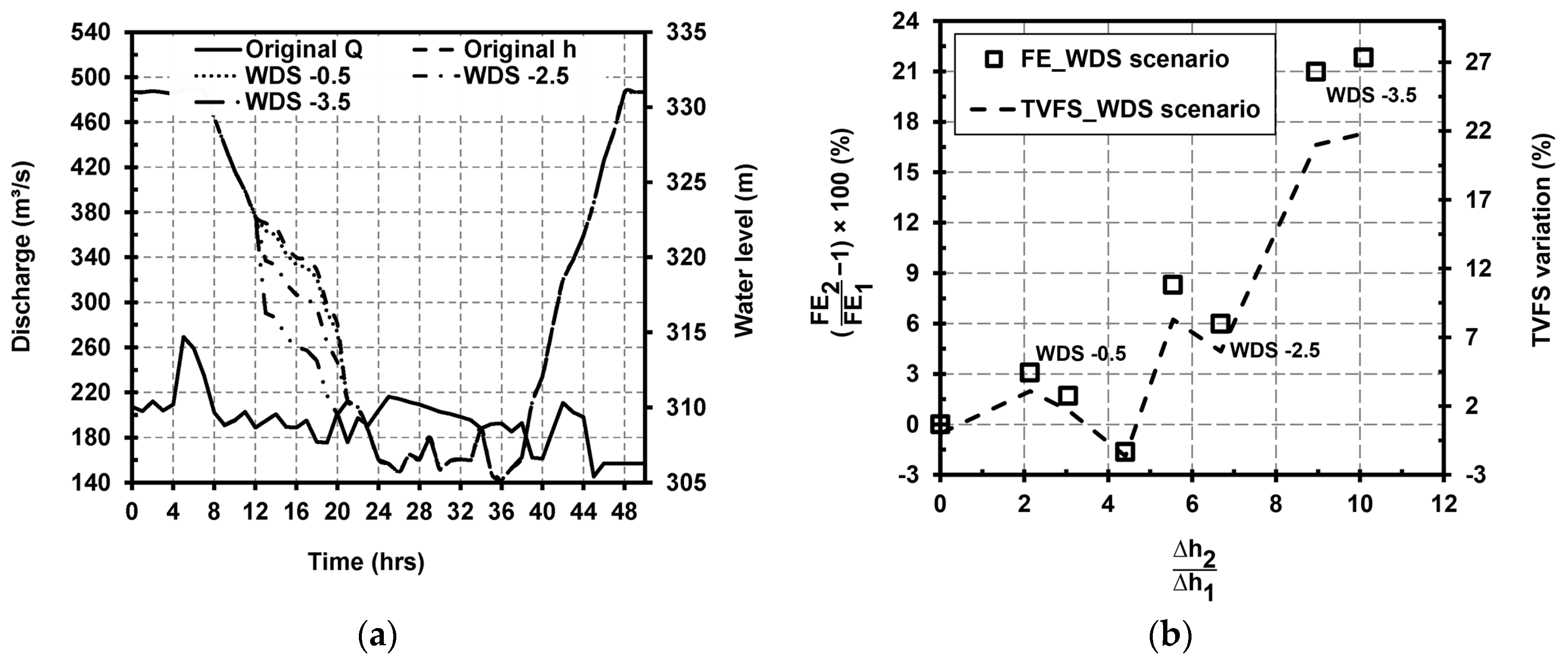
5.1.2. Water Level Scenarios

Dominant role of the water-level drawdown stage in scouring the flushing channel has been already highlighted in physical model studies [30,44]. Therefore, another feasible scenario for the Dashidaira reservoir is increasing the Water-level Drawdown Speed (i.e., the WDS scenario). A target limb during the second half of the drawdown stage (i.e., between t = 12 and 20 h after starting the flushing) in the water-level variation curve is selected. Then, the original water-level drawdown rate is increased significantly for 1 hour at the beginning of the target limb (i.e., between t = 12 and 13 h after starting the flushing). Afterwards, the original drawdown rates remain unchanged during the remaining time (i.e., from t = 13 until t = 20 h). As a result, introducing an extra drop in the water level (e.g., 0.5, 2.5, and 3.5 m) for one hour while the original discharge rates remain unchanged causes the water velocity to increase abruptly, which acts as a strong driving force over the bed materials. For example, the WDS −0.5 scenario represents an extra 0.5-m drop in the water level at the beginning of the relevant limb (i.e., between t = 12 and 20 h). This scenario can be created via gate operations during a flushing event (e.g., a temporary increase in the gate opening speed) or with modification of the bottom outlet geometry to increase the discharge capacity of the bottom outlets, which can contribute to a faster drawdown process. Figure 7a illustrates the original water level and discharge rates, together with water-level modifications, during the target limb for three different WDS scenarios in the Dashidaira reservoir.
The effects of introducing a faster drawdown of the water level on the FE and the TVFS under various WDS scenarios are shown in Figure 7b. The horizontal axis shows the ratio of the extra imposed water level drop (i.e., ∆h2) to the original one (i.e., ∆h1) at the beginning of the target limb during the drawdown stage. On the left vertical axis, FE2 represents the flushing efficiency when a WDS scenario is employed, and FE1 represents the flushing efficiency when the original water level of the 2012 flushing operation is applied. All calculated and presented values are relative to the reference case (i.e., the 2012 flushing operation). As shown in Figure 7b, the FE variations are overall directly related to the variations in ∆h2/∆h1. However, removing the coarser material from the far upstream area of the reservoir requires a high extra drop in the water level (i.e., a high ∆h2/∆h1). Moreover, in some cases, increasing ∆h2/∆h1 results in lower TVFS and FE values because coarser eroded material moves from upstream areas to downstream areas and is deposited on finer materials in the deeper areas. If the driving forces produced by the extra drop in the water level are not strong enough to remobilize the newly deposited coarser sediments overlying finer sediments, the erosion of finer fractions may be lower, resulting in lower TVFS values and consequently lower FE2 values. Table 3 also shows the average BCI values in the upstream, midstream and downstream areas of the Dashidaira reservoir after the application of the WDS −0.5, WDS −2.5, and WDS −3.5 scenarios. As shown in Table 3, compared to the reference case with the TVFS of 313.0 × 10³ m3, the TVFS increases slightly when the magnitude of the extra drop in the water level is small (e.g., 0.5 m in the WDS −0.5 scenario). When the extra drop in the water level is larger (e.g., 2.5 m), the TVFS increases but not remarkably. Although the water-level decrease can enhance the relative roughness (i.e., the ratio of the roughness height to the water depth), this increased roughness is not high enough to lead to the erosion of the coarser materials in the upstream areas. Thus, the main effect is limited to the finer materials in the WDS −0.5 and WDS −2.5 scenarios. Due to the larger extra water level drop in the WDS −3.5 scenario, higher bed erosion occurs over the entire reservoir, including the upstream areas covered with coarser materials. In Figure 5, the bed changes in different cross-sections located in areas I, II, and III under the WDS −3.5 scenario are compared to the bed levels in the reference simulations.
Although a marked drop in the water level enhances the sediment erosion from the entire reservoir area and increases the FE more than 20% as shown in Figure 7b, the flushing channel location remains close to the right bank in area II, and the deposits along the left bank (i.e., the dead zone) are not effectively removed. However, constraints imposed by the gate facilities for safe and quick opening, and existing risks regarding the side bank failures are necessary to be assessed carefully.

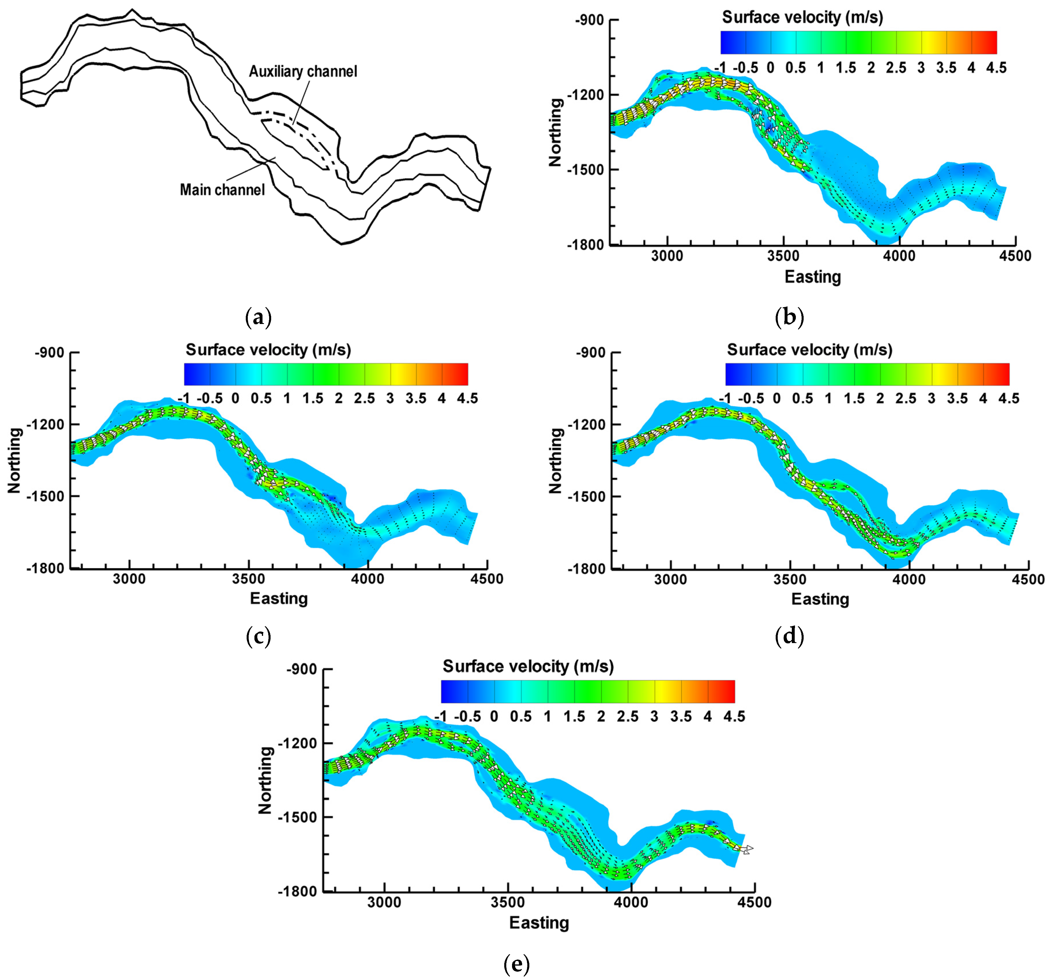
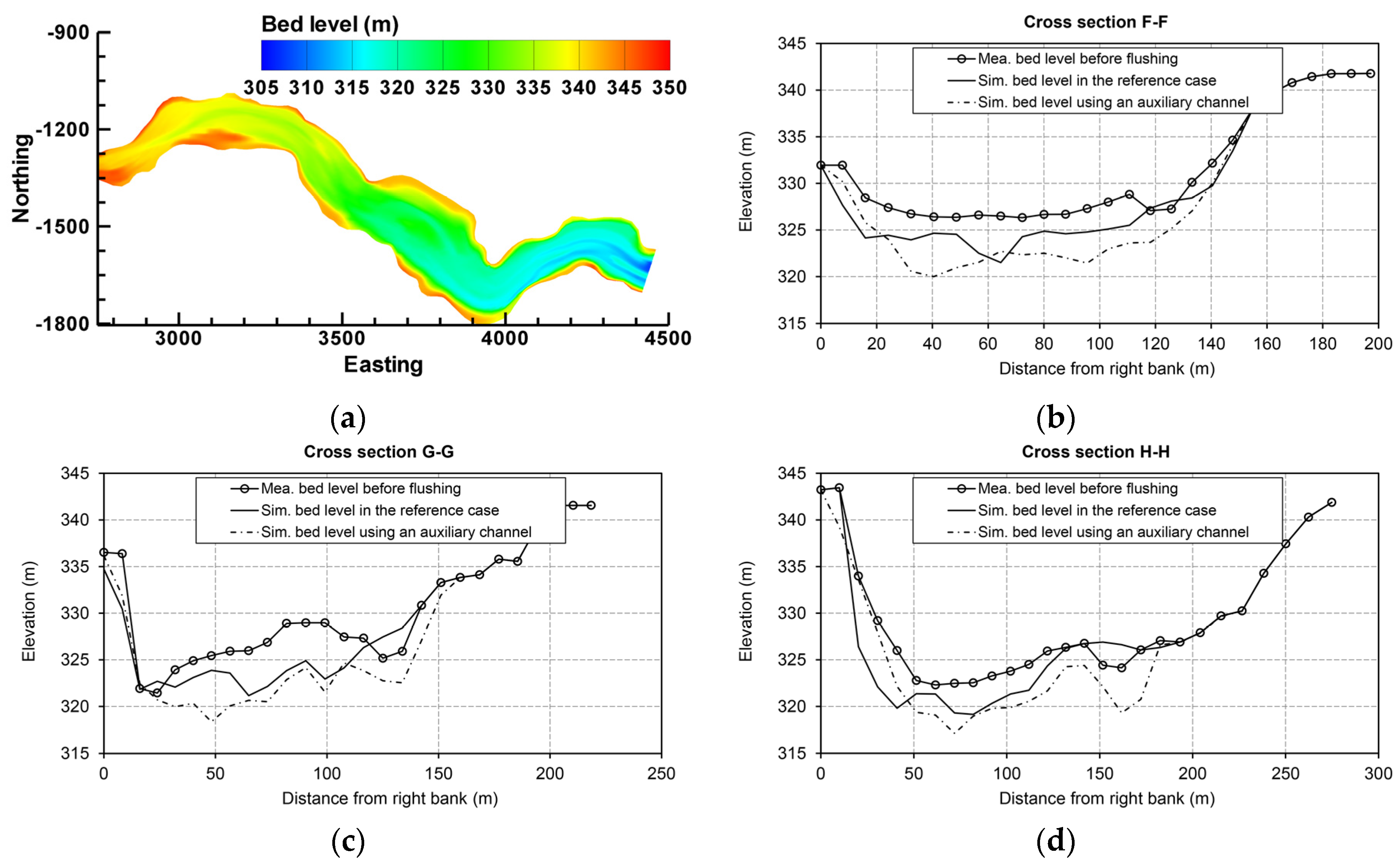
5.2. Auxiliary Channel Scenario

According to the literature, construction of longitudinal channels in the wide areas of the reservoir has been proposed for affecting the scouring pattern [4]. Thus, a potential scenario for improving the erosion in the dead zone area of the Dashidaira reservoir is the application of a longitudinal auxiliary (i.e., secondary) channel in the dead zone to act as a side channel beside the main channel. In this scenario, the flushing flow is partly diverted from the main channel into the auxiliary channel and enters the main channel again at a confluence further downstream of the diversion point. Thus, the morphological processes occur along two flushing channels in area II. In contrast to the discharge and water-level scenarios, which affect the hydrodynamic characteristics within the entire reservoir during the flushing operation, auxiliary channel scenario influences the hydrodynamic characteristics in a specific segment of the reservoir. Thus, the auxiliary channel scenario may be more useful for resolving the issue of ineffective sediment scouring within the dead zone area in the reservoir.
The presence of two flushing channels in area II is better than just one in terms of several aspects. First, erosion occurs in two flushing channels instead of one, which means that flushing occurs over a longer channel (i.e., larger area). Consequently, higher TVFS and FE values are expected. When a longitudinal auxiliary channel is not used, the flushing channel merely develops along the river thalweg (i.e., pre-existing flushing channel). The flushing channel attracts the entire flow, and the channel mainly deepens, which is not an effective approach for increasing the TVFS and FE. Second, a remarkable amount of previously unerodible sediments can be eroded from the dead zone following the construction of a longitudinal auxiliary channel.
The schematic illustration showing the location of the applied auxiliary channel and also the surface velocity vectors in different stages of the flushing using an auxiliary channel are shown in Figure 8. The location of the entrance of auxiliary channel was selected in a place where a portion of the flushing flow can be easily diverted into the channel (Figure 8a). In addition, in the numerical model, side banks of the auxiliary channel were implemented along the existing grid lines in the selected area of the dead zone. The depth and length of the channel were set to be 2.5 and 403 m, respectively. As shown in Figure 8b, the auxiliary channel deflects a portion of the water flow towards the dead zone, and the remaining flow continues its original path close to the right bank of area II along the original thalweg of the main flushing channel. At the beginning of the drawdown stage (i.e., t = 10 h) in Figure 8c, the incoming flow is mainly deflected towards the auxiliary channel. At the middle of the drawdown stage (i.e., t = 16 h), the flow bifurcates completely, with a major portion of the incoming flow being deflected towards the main channel and a smaller portion being deflected towards the auxiliary channel, as shown in Figure 8d. After erosion of the existing sandbar, between the main and auxiliary channel, and the consequent water exchange between the channels due to the small water level fluctuations during the free-flow stage, the water flow is distributed over a wider flushing channel. These conditions continue during the free-flow stage (i.e., t = 32 h), as shown in Figure 8e. More specifically, using a longitudinal auxiliary channel along the dead zone develops another thalweg away from the main flushing channel thalweg by attracting a portion of the incoming flow and preventing the entire flow from heading towards the right bank of area II.
Figure 9a illustrates the plan view of the final bed morphology in the scenario with an auxiliary longitudinal channel in the dead zone of area II. Utilizing this scenario increases the TVFS to 340.0 × 10³ m3, compared to the 313.0 × 10³ m3 of the reference case. In Figure 9b–d, the final bed levels in different cross-sections of area II are shown after the flushing operation and are compared to the bed levels in the reference case. One can clearly see that the bed levels decreased noticeably along the thalweg of the auxiliary flushing channel and meanwhile the channel widened. Both deepening and widening process of the auxiliary channel contributes in increasing the TVFS and subsequently the flushing efficiency.

6. Conclusions

The following results were obtained from the present work:
  • Both the MPM and Van Rijn formulas yielded satisfactory performances in the simulation of bed changes in specific segments of the reservoir during the flushing operation (e.g., MPM formula in the upper half of the reservoir and Van Rijn formula in the vicinity of the Dam). These sediment transport formulas have been developed empirically to calculate the sediment transport for a given set of sediment sizes and hydrodynamic boundary conditions. However, the bed sediment size distribution, bed roughness, and hydrodynamic boundary conditions change dynamically during the free-flow flushing process. Such significant changes cannot be handled by empirical sediment transport formulas due to their inherent limitations. Nevertheless, the MPM bed load sediment transport formula qualitatively and quantitatively performed better than the Van Rijn formula for the entire reservoir. The MPM formula was able to achieve TVFS values that were more than 75% that of the measured TVFS values. Due to the application of the empirical formulas, the alluvial roughness also could not be estimated appropriately, which further magnifies the mentioned inability of the sediment transport formulas to accurately represent the morphological bed changes.
  • For the Dashidaira reservoir, introducing an artificial additional discharge during the free-flow stage is practically feasible since this discharge can be supplied from upstream reservoirs. In addition, because this additional discharge is introduced when the flushing gates are fully opened and the water level is low, this discharge can be passed through the bottom outlets if its value is less than the maximum capacity of the outlets. Additional discharge has two major effects: first, it increases the induced bed shear stress and bed erosion and supplies an additional driving force to transport eroded sediments farther downstream in the reservoir and flush them out from the reservoir; second, it causes the water level to increase in the downstream river channel, which can be beneficial from an environmental point of view because it washes away fine materials from the downstream channel terraces (thereby preventing river channel clogging). However, it was found that introducing the extra discharge in the form of two discharge pulses with a larger discharge pulse in the second half of the free-flow stage more efficiently increases the FE ratio and the bed degradation in the upstream areas covered with coarser materials. The numerical outcomes showed that introducing approximately 21% more water from upstream reservoirs (i.e., an approximately 56% increase in the average free-flow discharge) can enhance the FE by approximately 5−13% compared to the reference case (i.e., the 2012 flushing operation), depending on how this additional discharge is delivered.
  • The construction of an auxiliary longitudinal flushing channel in the dead zone area of the Dashidaira reservoir causes a portion of the flushing flow to deviate from the main channel into the auxiliary channel and to enter the main channel again via a confluence downstream of the diversion point. The non-diverted flow continues along its original path along the thalweg of the main flushing channel and the diverted flow towards the auxiliary channel scour the deposited sediments from the targeted dead zone in the reservoir. The flushing processes associated with the auxiliary longitudinal channel result in a flushing channel that is overall longer and wider. Hence, the FE is higher by as much as approximately 9% compared to the reference case.

Acknowledgments

The first author was funded by the Ministry of Education, Culture, Sports, Science, and Technology of Japan (MEXT) through the HSE program for Asian Megacities. The support of the Disaster Prevention Research Institute (DPRI) of Kyoto University for open access publication is acknowledged. Authors would like to give their thanks to Kansai Electric Power Co., Inc., NEWJEC Inc., and also Shuhei Minami for providing the field data used in this study framework.

Author Contributions

Taymaz Esmaeili analyzed and processed the data, performed the numerical model tests and prepared the first and final draft of this manuscript. Tetsuya Sumi, Sameh A. Kantoush, Stefan Haun, and Nils Rüther provided their theoretical and practical insights and expertise on the outcomes and also contributed to preparation of the manuscript with reading and corrections. Yoji Kubota contributed to preparation and interpretation of a part of input and output data in the numerical model development stage.

Conflicts of Interest

The authors declare no conflict of interest. The funding sponsors had no role in the design of the study; in the collection, analyses, or interpretation of data; in the writing of the manuscript, and in the decision to publish the results.

References

  1. Kondolf, G.M.; Gao, Y.; Annandale, G.W.; Morris, G.L.; Jiang, E.; Zhang, J.; Cao, Y.; Carling, P.; Fu, K.; Guo, Q.; et al. Sustainable sediment management in reservoirs and regulated rivers: Experiences from five continents. Earth’s Future 2014, 2, 256–280. [Google Scholar] [CrossRef]
  2. Morris, G.L. Chapter 5: Sediment management and sustainable use of reservoirs. In Modern Water Resources Engineering; Wang, L.K., Yang, C.T., Eds.; Humana Press: Totowa, NJ, USA, 2014; Volume 15, pp. 279–337. [Google Scholar]
  3. White, R. Evacuation of Sediments from Reservoir; Thomas Telford: London, UK, 2001. [Google Scholar]
  4. Morris, G.L.; Fan, J. Reservoir Sedimentation Handbook: Design and Management of Dams, Reservoirs and Watersheds for Sustainable Use; McGraw-Hill: New York, NY, USA, 1998. [Google Scholar]
  5. Shen, H.W. Flushing sediment through reservoirs. J. Hydraul. Res. 1999, 37, 743–757. [Google Scholar] [CrossRef]
  6. Sumi, T.; Kantoush, S.A. Integrated management of reservoir sediment routing by flushing, replenishing, and bypassing sediments in Japanese river basins. In Proceedings of the 8th International Symposium on Ecohydraulics, Seoul, Korea, 12–16 September 2010. [Google Scholar]
  7. Liu, J.; Minami, S.; Otsuki, H.; Liu, B.; Ashida, K. Prediction of concerted sediment flushing. J. Hydraul. Eng. 2004, 130, 1089–1096. [Google Scholar] [CrossRef]
  8. Kantoush, S.A. Experimental Study on the Influence of the Geometry of Shallow Reservoirs on Flow Patterns and Sedimentation by Suspended Sediments. Ph.D. Thesis, Écolé Polytechnique Fédérale de Lausanne, Lausanne, Switzerland, 2008. [Google Scholar]
  9. Sloff, C.J.; Jagers, H.R.A.; Kitamura, Y. Study on the channel development in a wide reservoir. In Proceedings of the 2nd River Flow conference, Napoli, Italy, 23–25 June 2004. [Google Scholar]
  10. Fukuoka, S.; Sumi, T.; Horiuchi, S. Sediment management on the arase dam removal project. In Proceedings of the 12th International Symposium on River Sedimentation, Kyoto, Japan, 2–5 September 2013. [Google Scholar]
  11. Asahi, K.; Shimizu, Y.; Nelson, J.; Parker, G. Numerical simulation of river meandering with self-evolving banks. J. Geophysic. Res. 2013, 118, 2208–2229. [Google Scholar] [CrossRef]
  12. Fukuoka, S.; Uchida, T. Toward integrated multi-scale simulations of flow and sediment transport in rivers. J. Jpn. Soc. Civ. Eng. 2013, 69, II_1–II_10. [Google Scholar] [CrossRef]
  13. Fang, H.; Rodi, W. Three-dimensional calculation of flow and suspended sediment transport in the neighbourhoods of the dam for the Three Gorges Project (TGP) reservoir in the Yangtze River. J. Hydraul. Res. 2003, 41, 379–394. [Google Scholar] [CrossRef]
  14. Lu, Y.J.; Wang, Z.Y. 3D numerical simulation for water flows and sediment deposition in dam areas of the Three Gorges project. J. Hydraul. Eng. 2009, 135, 755–769. [Google Scholar] [CrossRef]
  15. Haun, S.; Olsen, N.R.B. Three-dimensional numerical modelling of the flushing process of the Kali Gandaki hydropower reservoir. Lakes Reserv. 2012, 17, 25–33. [Google Scholar] [CrossRef]
  16. Khosronejad, A.; Rennie, C.D.; Salehi Neyshabouri, A.A.; Gholam, I. Three-dimensional numerical modeling of reservoir sediment release. J. Hydraul. Res. 2008, 46, 209–223. [Google Scholar] [CrossRef]
  17. Harb, G.; Dorfmann, C.; Schneider, J.; Badura, H. Numerical analysis of sediment transport processes during a flushing event of an Alpine reservoir. In Proceedings of the 7th River Flow conference, Lausanne, Switzerland, 3–5 September 2014. [Google Scholar]
  18. Gallerano, F.; Cannata, G. Compatibility of Reservoir Sediment Flushing and River Protection. J. Hydraul. Eng. 2011, 137, 1111–1125. [Google Scholar] [CrossRef]
  19. Haun, S.; Olsen, N.R.B. Three-dimensional numerical modelling of reservoir flushing in a prototype scale. Int. J. River Basin Manag. 2012, 10, 341–349. [Google Scholar] [CrossRef]
  20. Olsen, N.R.B. A Three Dimensional Numerical Model for Simulation of Sediment Movement in Water Intakes with Multiblock Option; Department of Hydraulic and Environmental Engineering, The Norwegian University of Science and Technology: Trondheim, Norway, 2014. [Google Scholar]
  21. Esmaeili, T.; Sumi, T.; Kantoush, S.A.; Haun, S.; Rüther, N. Three-dimensional numerical modelling of flow field in shallow reservoirs. Proc. ICE-Water Manag. 2015, 169, 229–244. [Google Scholar] [CrossRef]
  22. Dehghani, A.A.; Esmaeili, T.; Chang, W.Y.; Dehghani, N. 3D numerical simulation of local scouring under hydrographs. Proc. ICE-Water Manag. 2013, 166, 120–131. [Google Scholar] [CrossRef]
  23. Haun, S.; Kjærås, H.; Løvfall, S.; Olsen, N.R.B. Three-dimensional measurements and numerical modelling of suspended sediments in a hydropower reservoir. J. Hydrol. 2013, 479, 180–188. [Google Scholar] [CrossRef]
  24. Esmaeili, T.; Dehghani, A.A.; Zahiri, A.R.; Suzuki, K. 3D Numerical simulation of scouring around bridge piers (Case Study: Bridge 524 crosses the Tanana River). World Acad. Sci. Eng. Technol. 2009, 58, 1028–1032. [Google Scholar]
  25. Fischer-Antze, T.; Olsen, N.R.B.; Gutknecht, D. Three-dimensional CFD modeling of morphological bed changes in the Danube River. Water Resour. Res. 2008, 44. [Google Scholar] [CrossRef]
  26. Rüther, N.; Olsen, N.R.B. Modelling free-forming meander evolution in a laboratory channel using three-dimensional computational fluid dynamics. Geomorphology 2007, 89, 308–319. [Google Scholar] [CrossRef]
  27. Ruether, N.; Singh, J.M.; Olsen, N.R.B.; Atkinson, E. 3-D computation of sediment transport at water intakes. Proc. ICE-Water Manag. 2005, 158, 1–7. [Google Scholar] [CrossRef]
  28. Olsen, N.R.B.; Kjellesvig, H.M. Three-dimensional numerical modelling of bed changes in a sand trap. J. Hydraul. Res. 1999, 37, 189–198. [Google Scholar] [CrossRef]
  29. Haun, S.; Dorfmann, C.; Harb, G.; Olsen, N.R.B. Numerical modelling of the reservoir flushing of the bodendorf reservoir, Austria. In Proceedings of the 2nd IAHR European Congress, Munich, Germany, 27–29 June 2012. [Google Scholar]
  30. Esmaeili, T.; Sumi, T.; Kantoush, S.A. Experimental and numerical study of flushing channel formation in shallow reservoirs. J. Jpn. Soc. Civ. Eng. 2014, 70, I_19–I_24. [Google Scholar] [CrossRef]
  31. Kantoush, S.A.; Sumi, T.; Suzuki, T.; Murasaki, M. Impacts of sediment flushing on channel evolution and morphological processes: Case study of the Kurobe River, Japan. In Proceedings of the 5th River Flow Conference, Braunschweig, Germany, 8–10 June 2010. [Google Scholar]
  32. Minami, S.; Noguchi, K.; Otsuki, H.; Fukuri, H.; Shimahara, N.; Mizuta, J.; Takeuchi, M. Coordinated sediment flushing and effect verification of fine sediment discharge operation in Kurobe River. In Proceedings of the ICOLD Conference, Kyoto, Japan, 6–8 June 2012. [Google Scholar]
  33. Sumi, T. Evaluation of efficiency of reservoir sediment flushing in Kurobe River. In Proceedings of the 4th International Conference on Scour and Erosion, Tokyo, Japan, 5–7 November 2008. [Google Scholar]
  34. Launder, B.E.; Spalding, D.B. Lectures in Mathematical Models of Turbulence; Academic Press: London, UK, 1972. [Google Scholar]
  35. Patankar, S. Numerical Heat Transfer and Fluid Flow; Taylor & Francis: New York, NY, USA, 1980. [Google Scholar]
  36. Olsen, N.R.B.; Haun, S. Free surface algorithms for 3-D numerical modeling of flushing. In Proceedings of the 5th River Flow Conference, Braunschweig, Germany, 8–10 June 2010. [Google Scholar]
  37. Schlichting, H. Boundary Layer Theory; McGraw-Hill: New York, NY, USA, 1979. [Google Scholar]
  38. Van Rijn, L.C. Sediment transport, part III: Bed forms and alluvial roughness. J. Hydraul. Eng. 1984, 110, 1733–1754. [Google Scholar] [CrossRef]
  39. Van Rijn, L.C. Sediment transport, part II: Suspended load Transport. J. Hydraul. Eng. 1984, 110, 1613–1641. [Google Scholar] [CrossRef]
  40. Van Rijn, L.C. Sediment transport, part I: Bed load transport. J. Hydraul. Eng. 1984, 110, 1431–1456. [Google Scholar] [CrossRef]
  41. Meyer-Peter, E.; Müller, R. Formulas for bed load transport. In Proceedings of the 2nd Meeting of the International Association for Hydraulic Structures Research, IAHR, Stockholm, Sweden, 7–9 June 1948. [Google Scholar]
  42. Brooks, H. Boundary shear stress in curved trapezoidal channels. J. Hydraul. Div. Am. Soc. Civ. Eng. 1963, 89, 327–333. [Google Scholar]
  43. Esmaeili, T.; Sumi, T.; Kantoush, S.A.; Kubota, Y.; Haun, S. Numerical study on flushing channel evolution, case study of Dashidaira reservoir, Kurobe river. J. Jpn. Soc. Civ. Eng. 2015, 71, I_115–I_120. [Google Scholar] [CrossRef]
  44. Kantoush, S.A.; Schleiss, A.J. Channel formation in large shallow reservoirs with different geometries during flushing. J. Environ. Technol. 2009, 30, 855–863. [Google Scholar] [CrossRef] [PubMed]
Figure 1. (a) Site map of the Kurobe River showing the location of the Dashidaira reservoir [31]; (b) Measured bed topography of the Dashidaira reservoir before the flushing operation in June 2012 and locations of the cross-sections A-L for further assessment of the bed variations in the upstream (i.e., area I), midstream (i.e., area II), and downstream (i.e., area III) portions of the reservoir; (c) Water level and discharge rates during the flushing operation in June 2012; (d) Onsite view of the dead zone area during the 2012 flushing operation (the dead zone area has been shown with ellipse dashed line and arrows show the flow direction).
Water 09 00900 g001
Figure 2. Computational grid (a1) at the beginning of the drawdown stage (t = 10 h) and (a2) during the free-flow condition in the Dashidaira reservoir (t = 32 h); corresponding surface velocity fields: (b1) at the beginning of the drawdown stage (t = 10 h) and (b2) during the free-flow condition (t = 32 h). The illustration on the right in (b1) shows the reverse flow domain and stagnant water zone.
Water 09 00900 g002
Figure 3. (a) Plan view of the measured bed topography after the 2012 flushing operation; Plan view of the simulated bed topography using (b) the MPM formula and (c) the Van Rijn formula.
Water 09 00900 g003
Figure 4. (a) Constant additional discharge rates used for different ADF scenarios in the Dashidaira reservoir. These additional rates are added to the original discharge rates shown in Figure 1c; (b) Modified hydrodynamic boundary conditions for different ADF scenarios in the Dashidaira reservoir; (c) Non-dimensional curves showing the relationships among TVFS, FE, and the water discharge used under different ADF scenarios compared to the reference case; (d) Schematic figure illustrating the PDF scenario with a variable discharge pulse in the second half of the free-flow stage.
Water 09 00900 g004
Figure 5. Measured bed levels before flushing along with the simulated bed levels after flushing in the reference case and under the ADF 110, ADF 170 and WDS −3.5 scenarios at (a1,a2) cross section A-A; (b1,b2) cross section E-E; (c1,c2) cross section F-F; (d1,d2) cross section H-H; (e1,e2) cross section K-K; and (f1,f2) cross-section L-L. Locations of the cross sections can be found in Figure 1b. Mea. and Sim. are abbreviations for Simulated and Measured, respectively.
Water 09 00900 g005aWater 09 00900 g005b
Figure 6. Measured bed levels before flushing and the simulated bed levels after flushing under the ADF 110 and PDF P1 110 8-P2 183.5 6 scenarios at (a) cross section A-A; (b) cross section B-B; (c) cross section C-C; (d) cross section D-D; and (e) cross section E-E. Locations of the sections can be found in Figure 1b.
Water 09 00900 g006
Figure 7. (a) Utilized water levels and discharge rates for different WDS scenarios; (b) Non-dimensional curves showing the relationship among TVFS, FE, and ∆h under different WDS scenarios compared to the reference case.
Water 09 00900 g007
Figure 8. (a) Schematic illustration of the concept of longitudinal auxiliary flushing channel in the dead zone area of the Dashidaira reservoir; The surface velocity field in different stages using an auxiliary flushing channel: (b) before onset of the drawdown stage (i.e., t = 5 h); (c) at the beginning of the drawdown stage (i.e., t = 10 h); (d) at the middle of the drawdown stage (i.e., t = 16 h); and (e) during the free-flow condition (i.e., t = 32 h).
Water 09 00900 g008
Figure 9. (a) Plan view of the final simulated bed levels using an auxiliary flushing channel along the dead zone of area II. Measured bed levels before flushing and simulated ones after flushing in the reference case along with simulated ones using an auxiliary flushing channel, at the location of (b) cross section F-F; (c) cross section G-G; (d) cross section H-H. Location of the cross sections can be found in Figure 1b.
Water 09 00900 g009
Table 1. Average sediment size distribution in the specified cross-sections shown in Figure 1b. Cs. is an abbreviation for Cross-section.
Sediment Size (mm)Cs. A-A (%)Cs. B-B (%)Cs. C-C (%)Cs. D-D (%)Cs. E-E (%)Cs. F-F (%)Cs. G-G (%)Cs. H-H (%)Cs. I-I (%)Cs. J-J (%)Cs. K-K (%)Cs. L-L (%)
316200000000000
118.374000000000040
37.467375706941000030
11.8476813145000016
3.7314111412251800003
1.2541322321061301
0.37627543555100948710010
Table 2. Sensitivity analysis of the TVFS in reference case with respect to the selected empirical parameters along with variation of the MAE of simulated bed levels for each case.
ParameterActive Layer Thickness (m)Water Content of the Bed Material(%)Critical Angle of Repose (Degree)
0.30.450.85504338333435
TVFS (×10−3 m3)261.6290.5299.8369.1306.2316.8311.0302.7284.5
MAE (m) 2.171.731.952.252.101.751.981.541.98
Table 3. Average bed level changes in different areas of the reservoir under different ADF, PDF, and WDS scenarios. For ADF and WDS scenarios, the simulated bed levels after 2012 flushing operation were used as the reference case to extract the BCI parameter, whereas for PDF scenario the simulated bed levels under the ADF 110 scenario were used as the reference case.
ScenarioADF 75ADF 110ADF 170
AreaIIIIIIIIIIIIIIIIII
BCI (m)0.32−0.47−0.540.06−0.49−0.550.20−0.76−0.90
TVFS (×10−3 m3)356.0396.1425.0
ScenarioPDF P1 110 8-P2 137.5 8PDF P1 110 8-P2 157 7PDF P1 110 8-P2 183.5 6
AreaIIIIIIIIIIIIIIIIII
BCI (m)−0.01−0.09−0.210.02−0.04−0.20−0.090.010.04
TVFS (×10−3 m3)426.2417.3410.9
ScenarioWDS −0.5WDS −2.5WDS −3.5
AreaIIIIIIIIIIIIIIIIII
BCI (m)0.03−0.140.020.10−0.13−0.23−0.08−0.33−0.22
TVFS (×10−3 m3)322.8331.9378.9

