SPH Modelling of Hydraulic Jump Oscillations at an Abrupt Drop


Abstract
1. Introduction
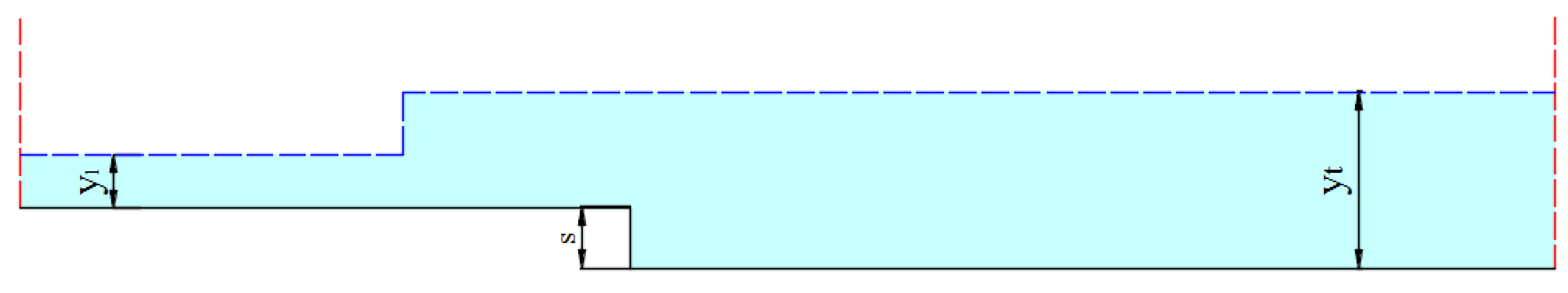
2. Experimental Set Up
3. SPH Numerical Method
- (1)
- (2)
- A SPH version of the standard k-ε turbulence model by [70], in which and the two equations for the turbulent kinetic energy k and for the turbulent dissipation rate ε are:where Pk is the production of turbulent kinetic energy depending on the local rate of deformation and νT is the eddy viscosity. As in [71], the values originally proposed by [70] for the model constants (σk = 1, σε = 1.3, Cε1 = 1.44, Ce2 = 1.92) were maintained here.
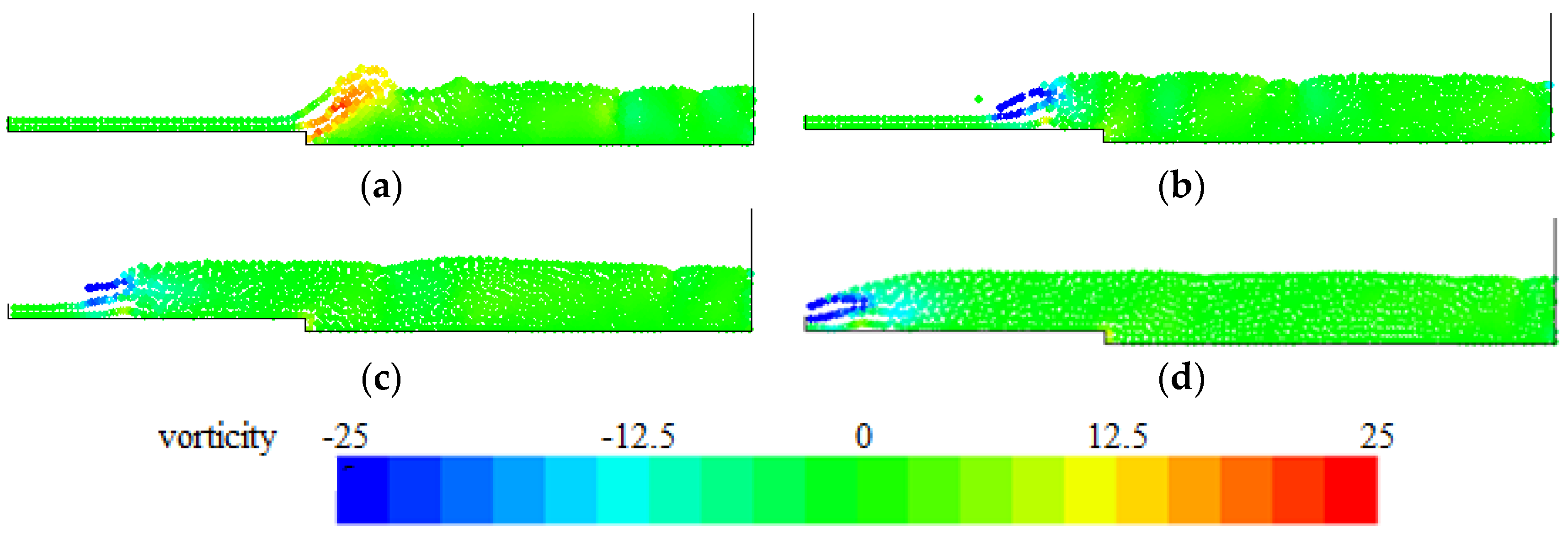
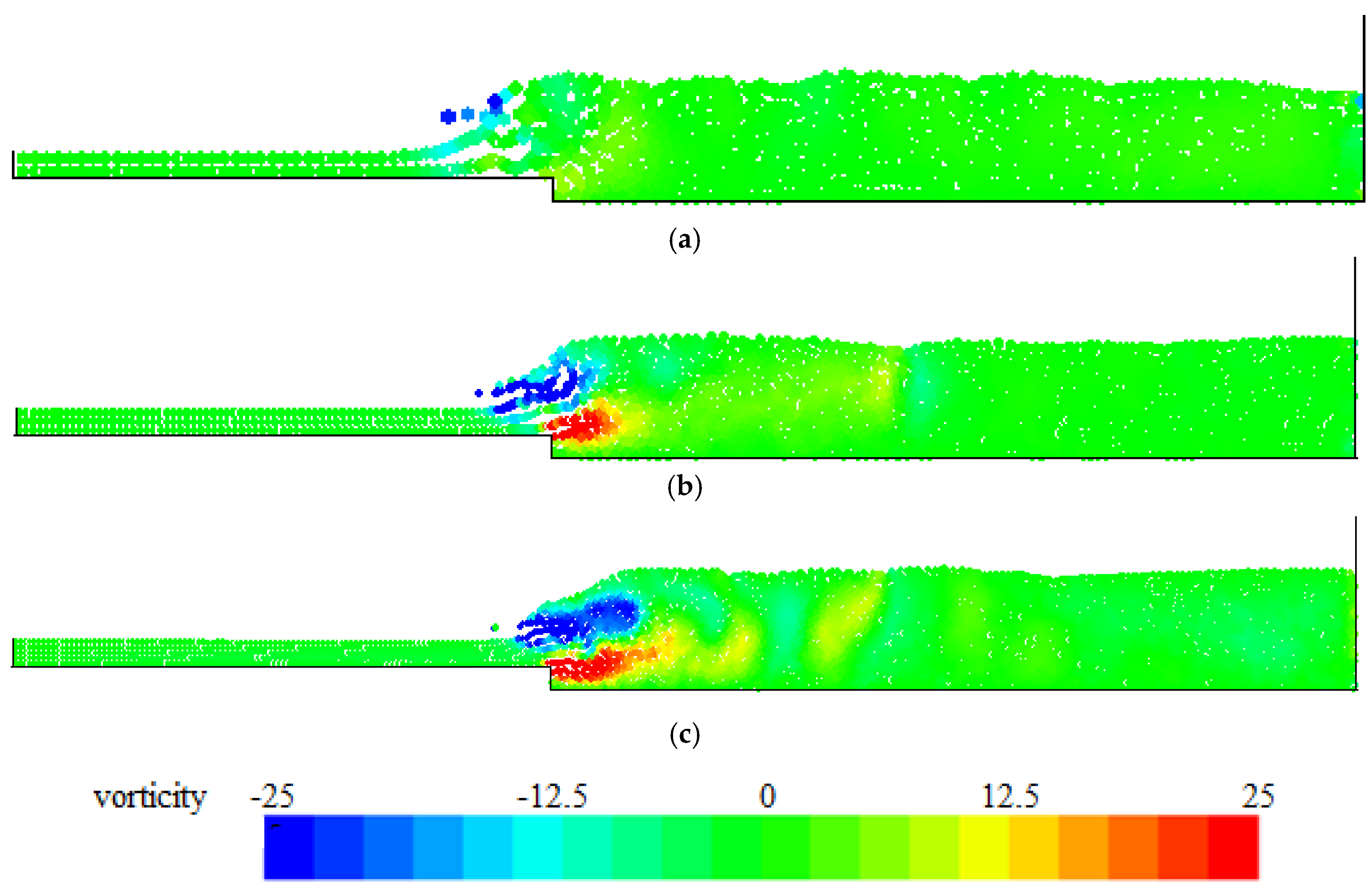
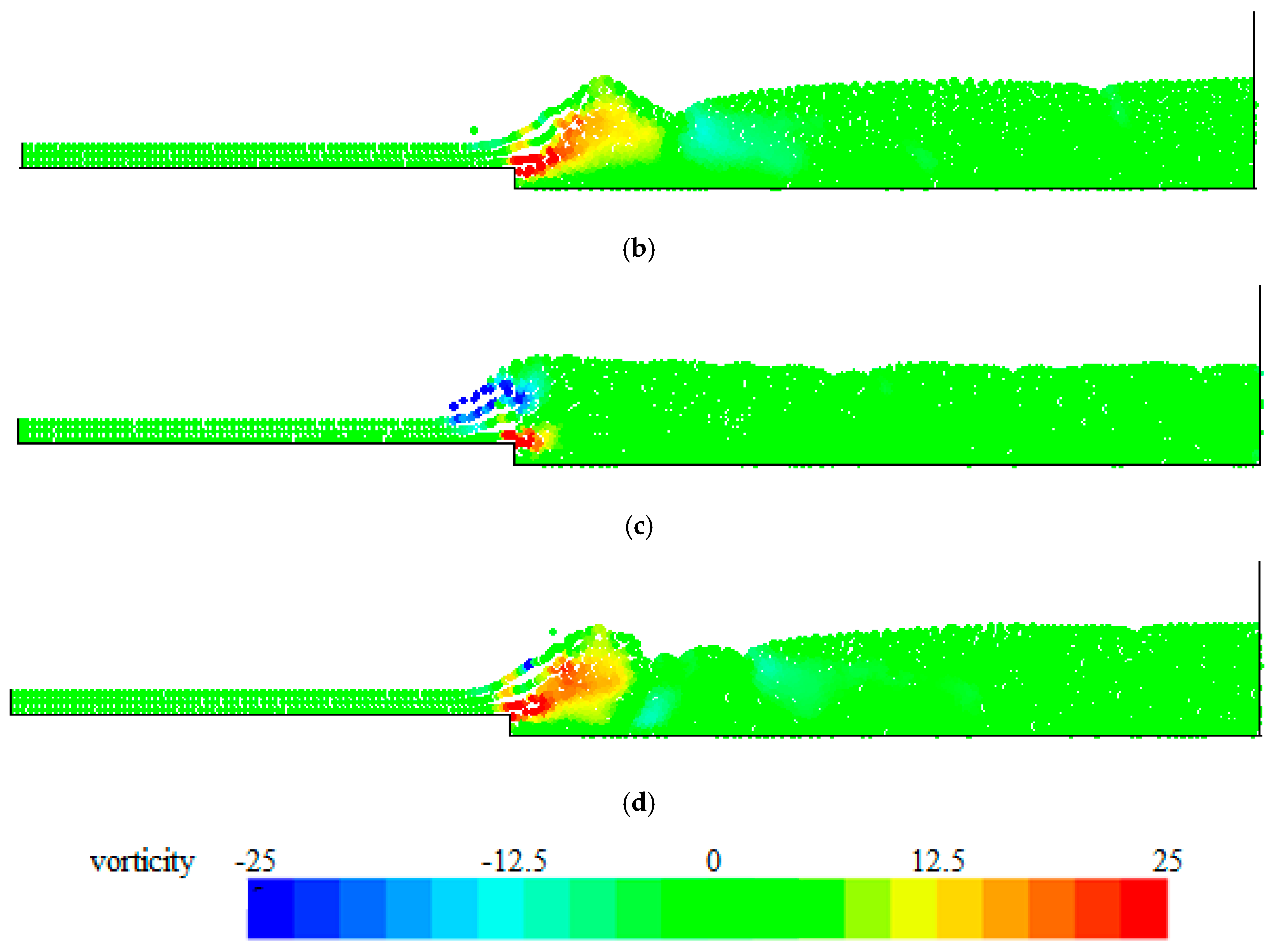
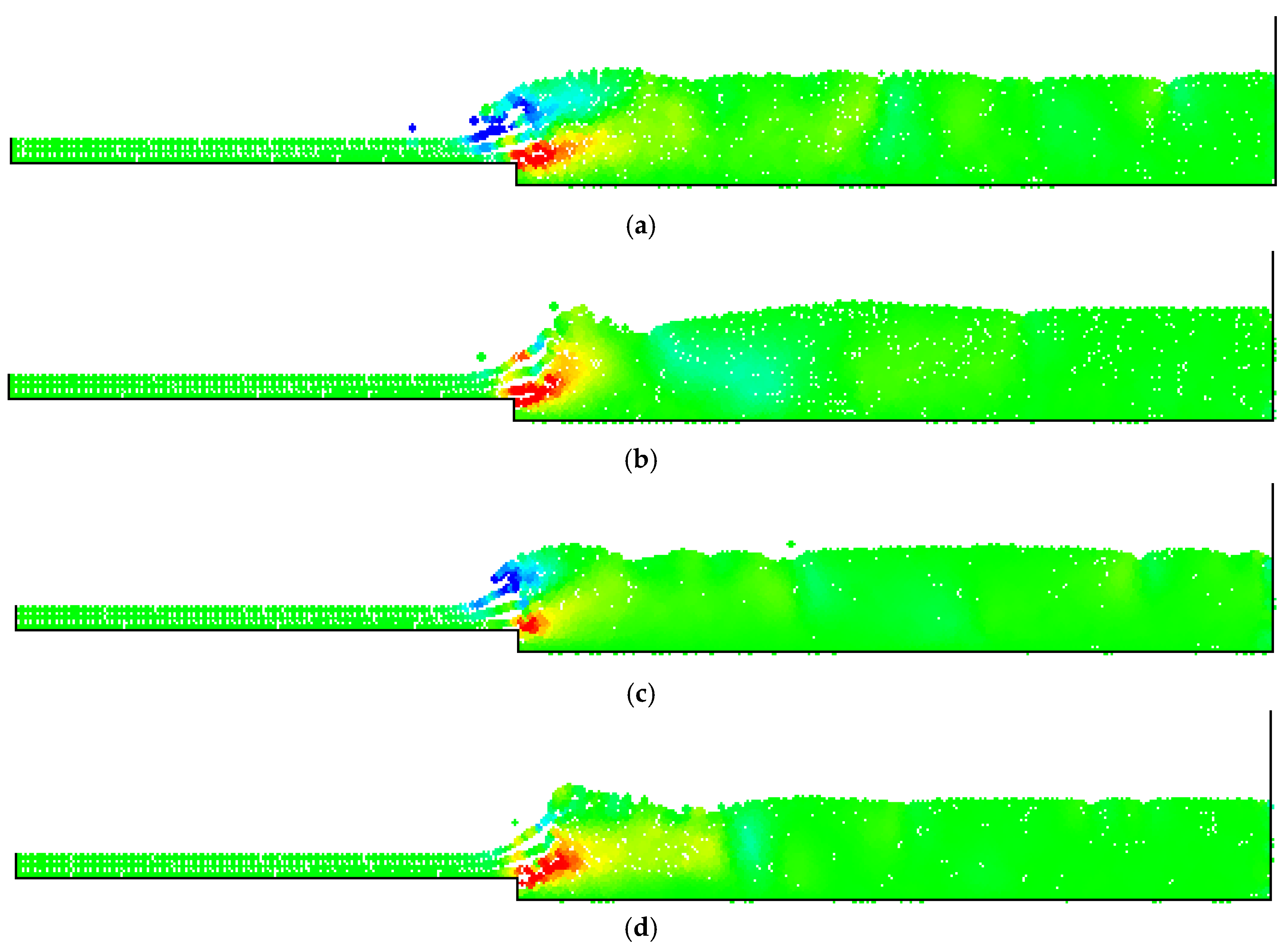
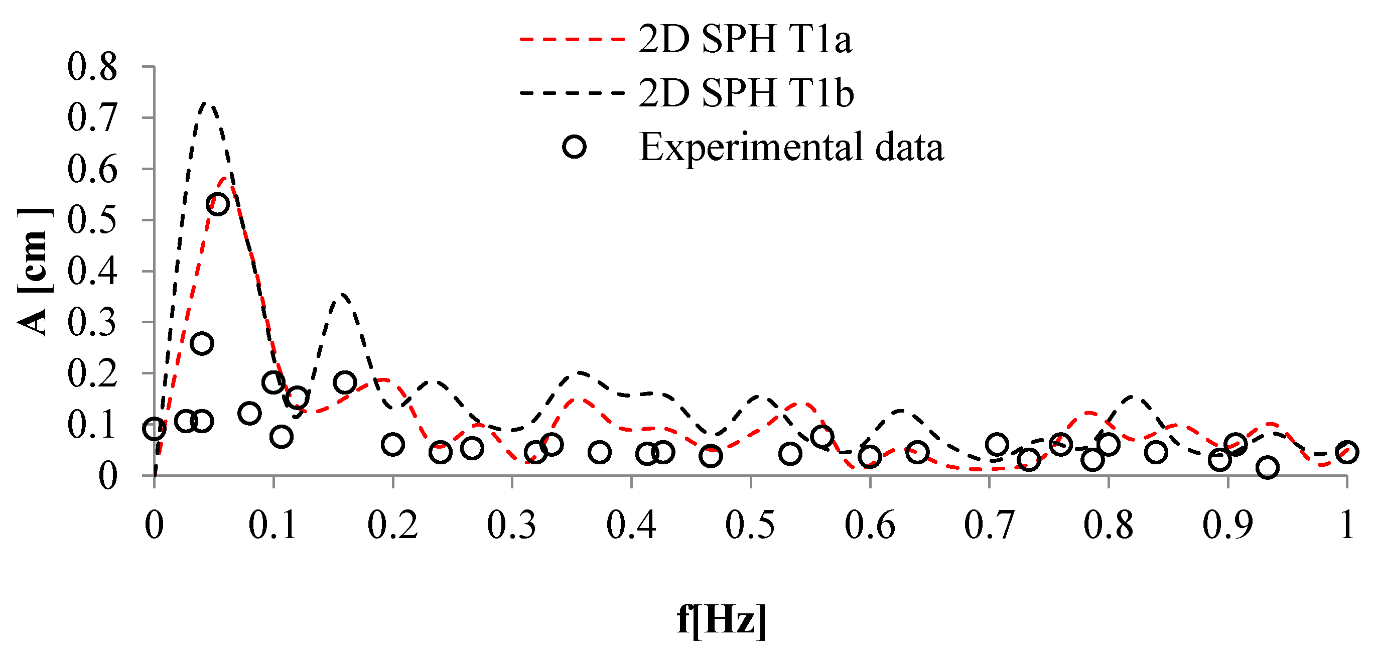
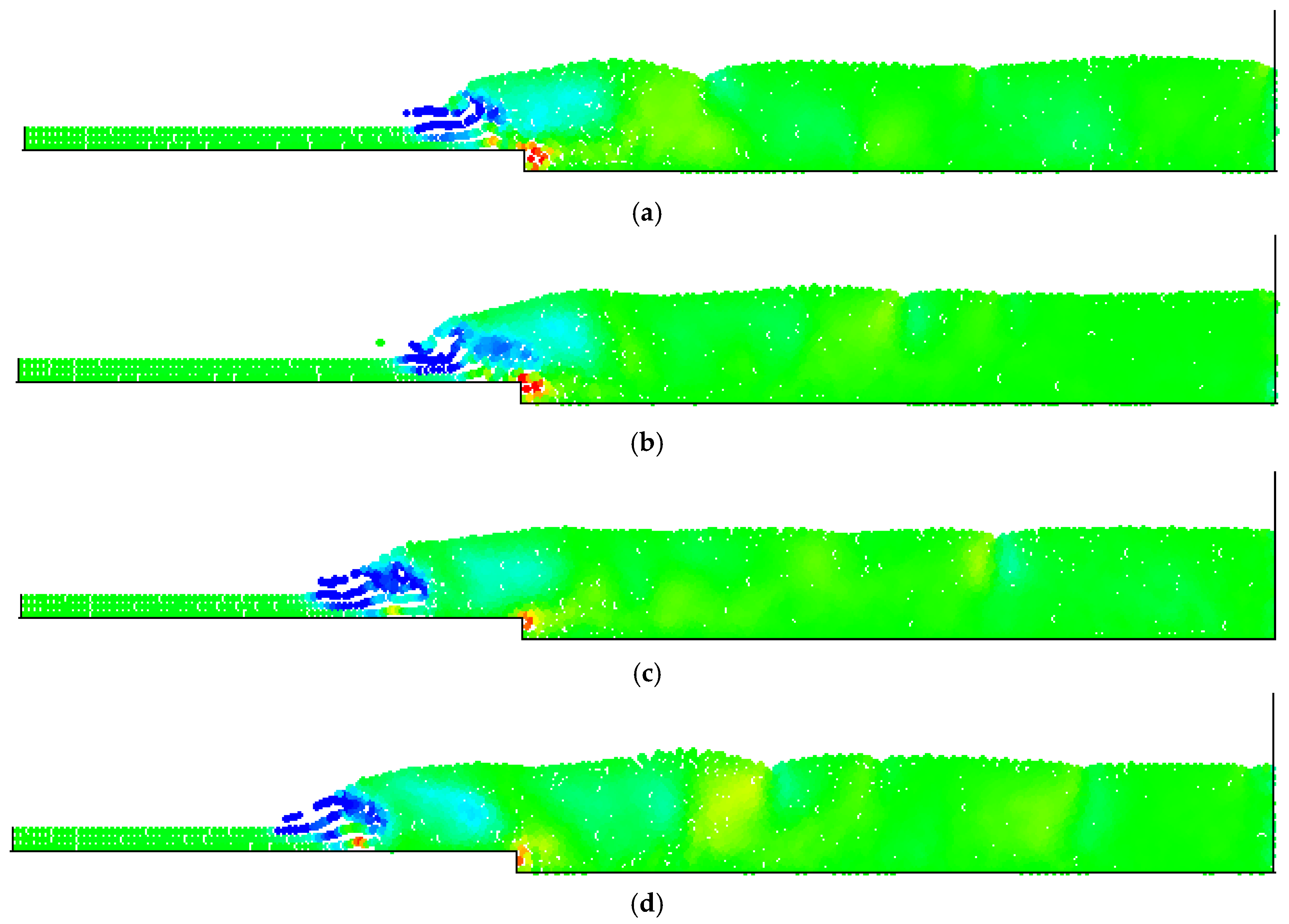
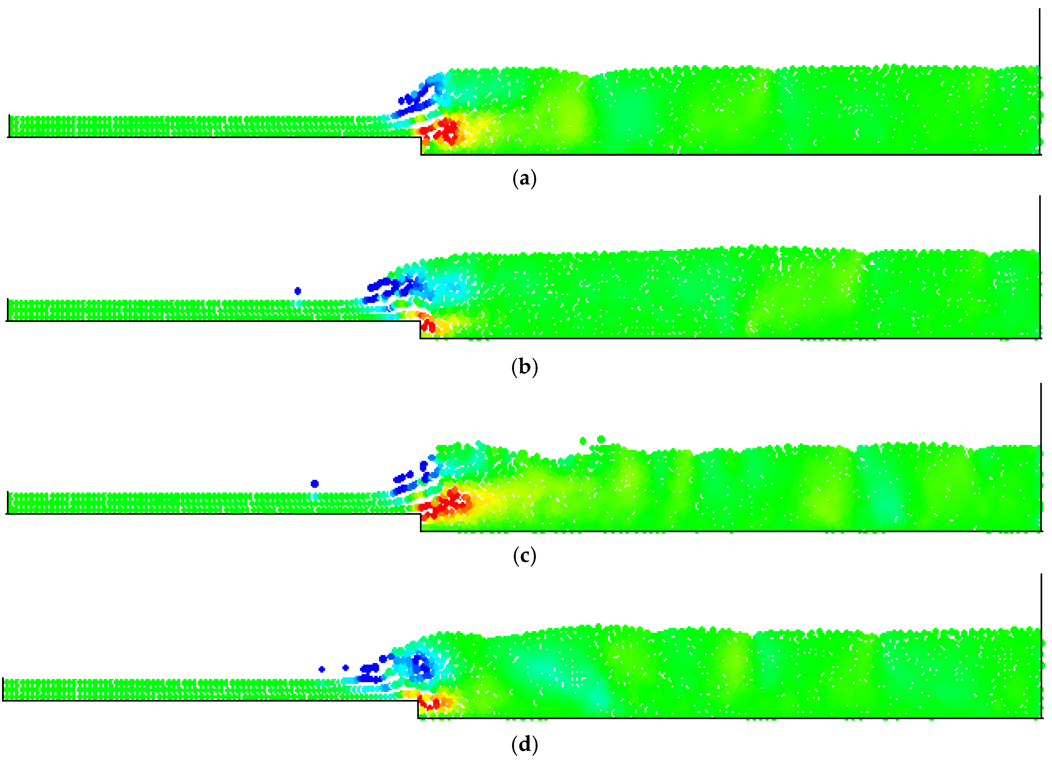
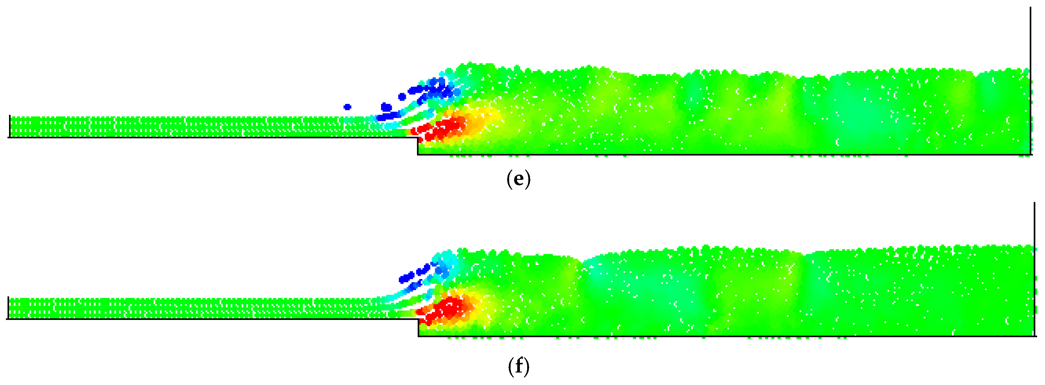
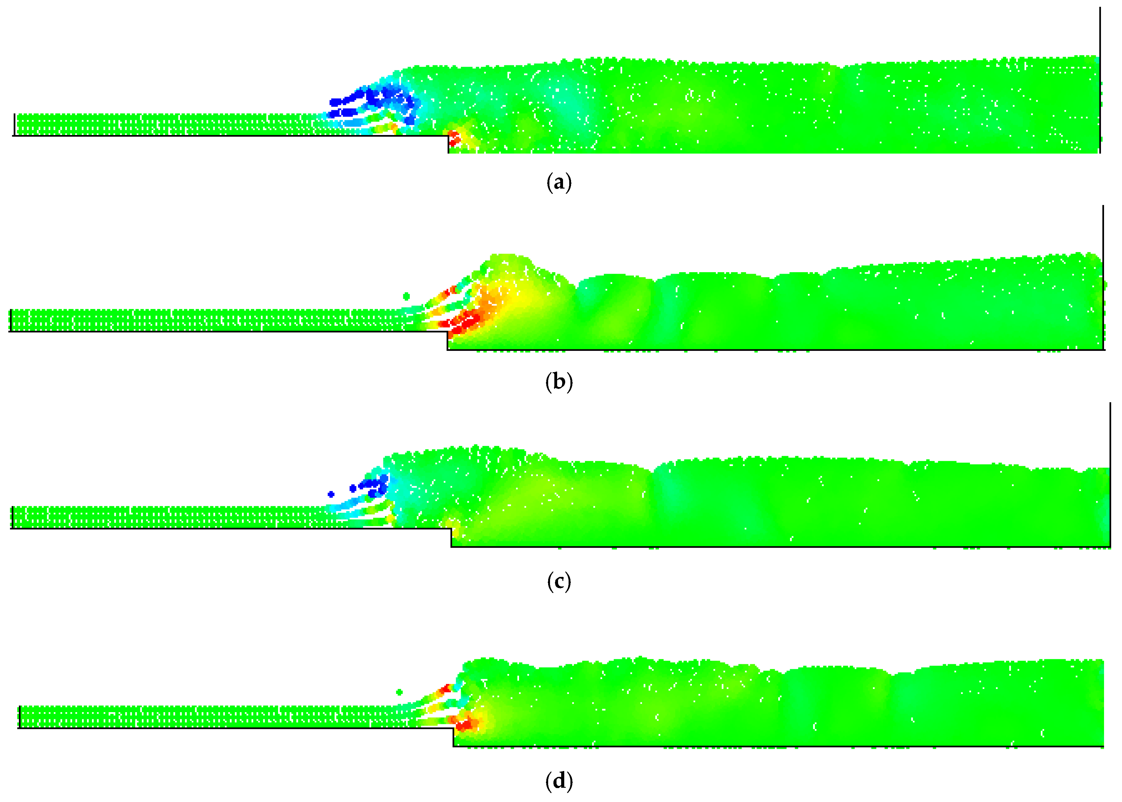
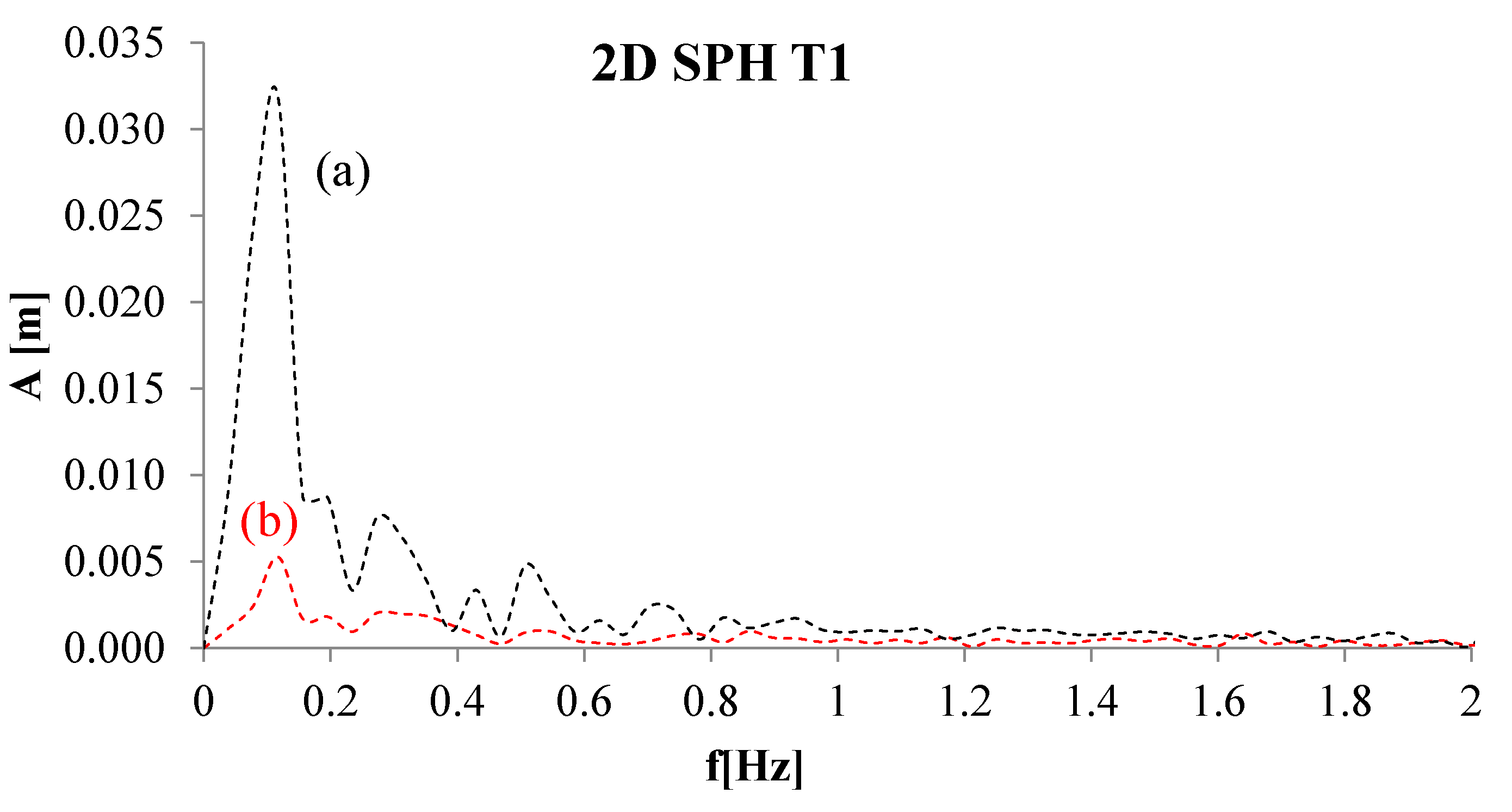
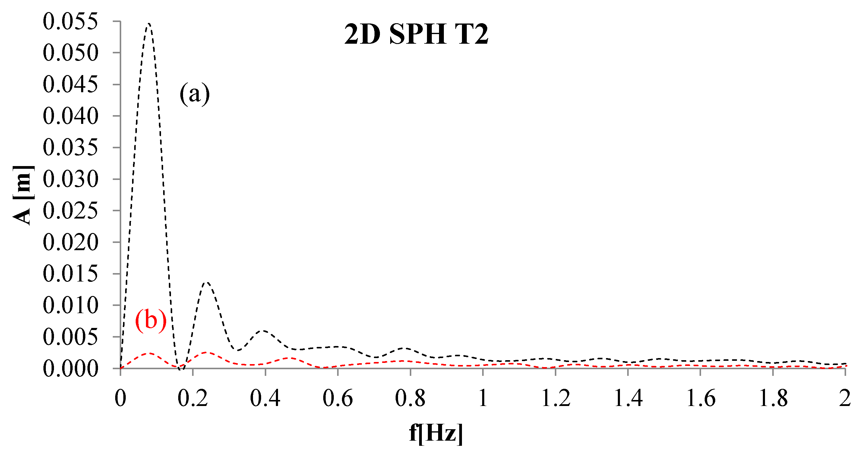
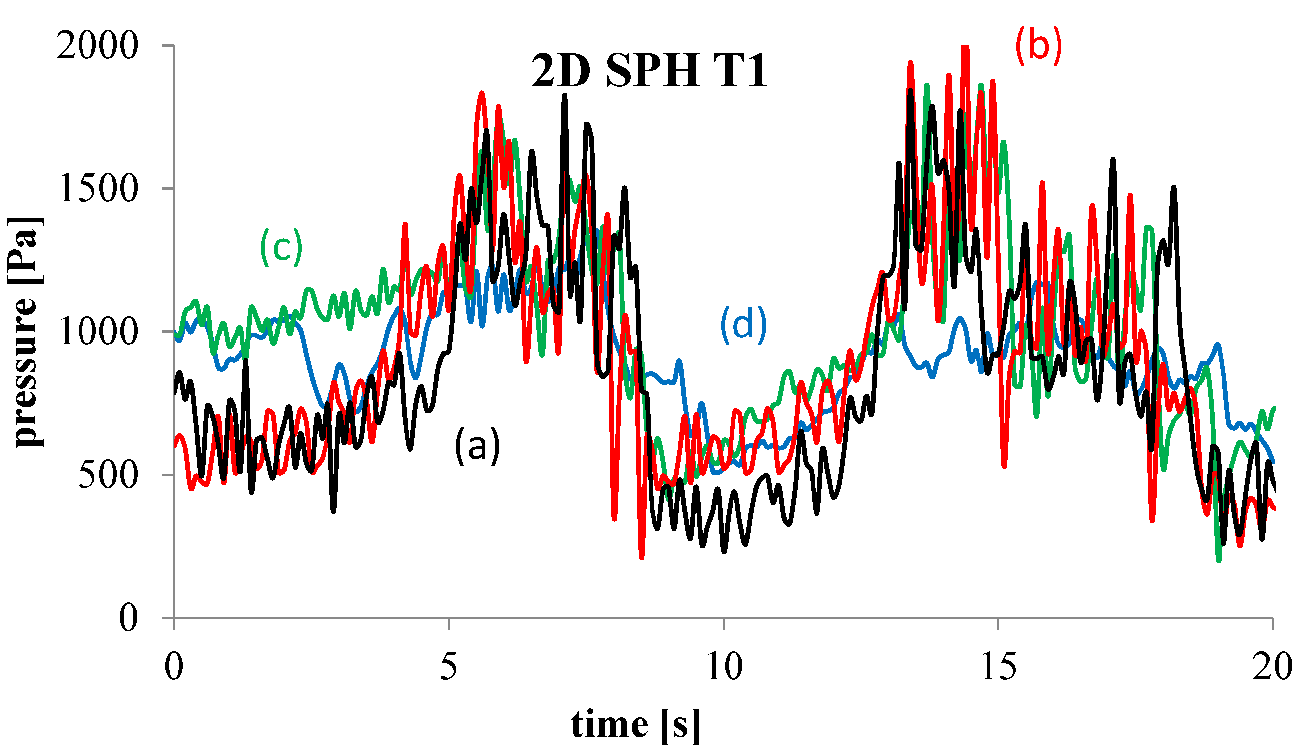
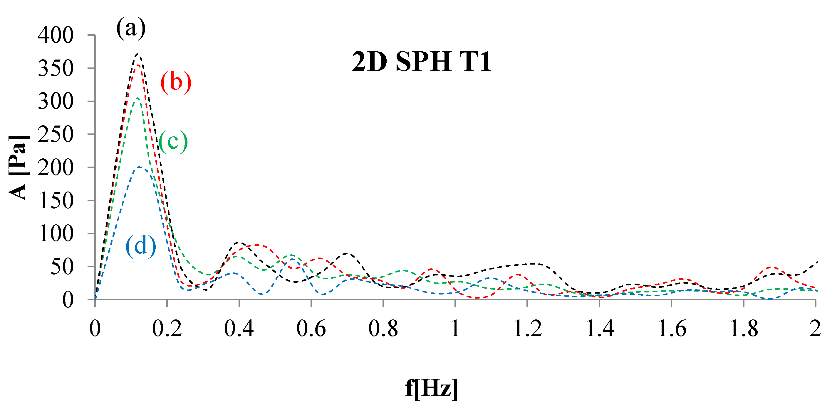
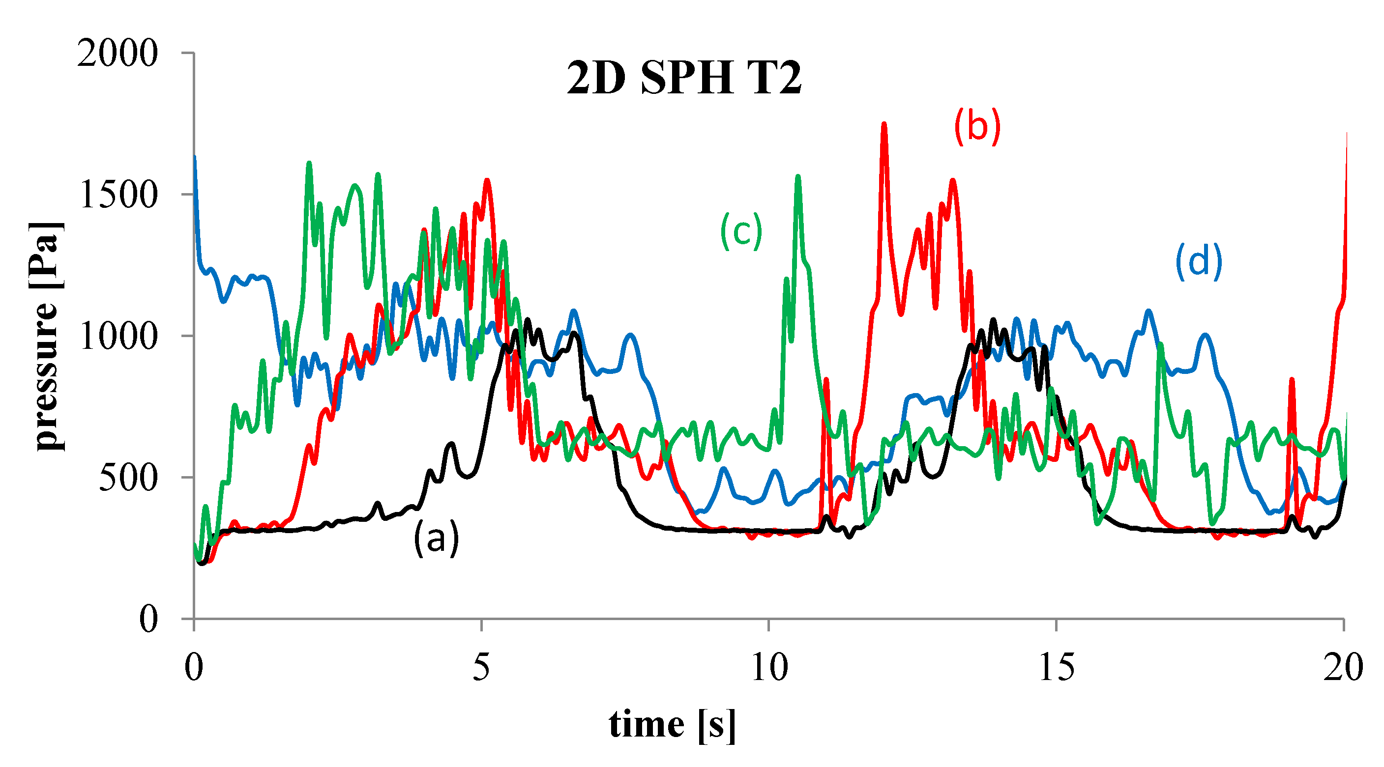
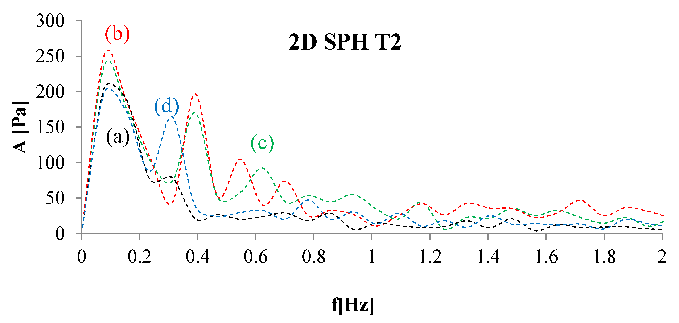
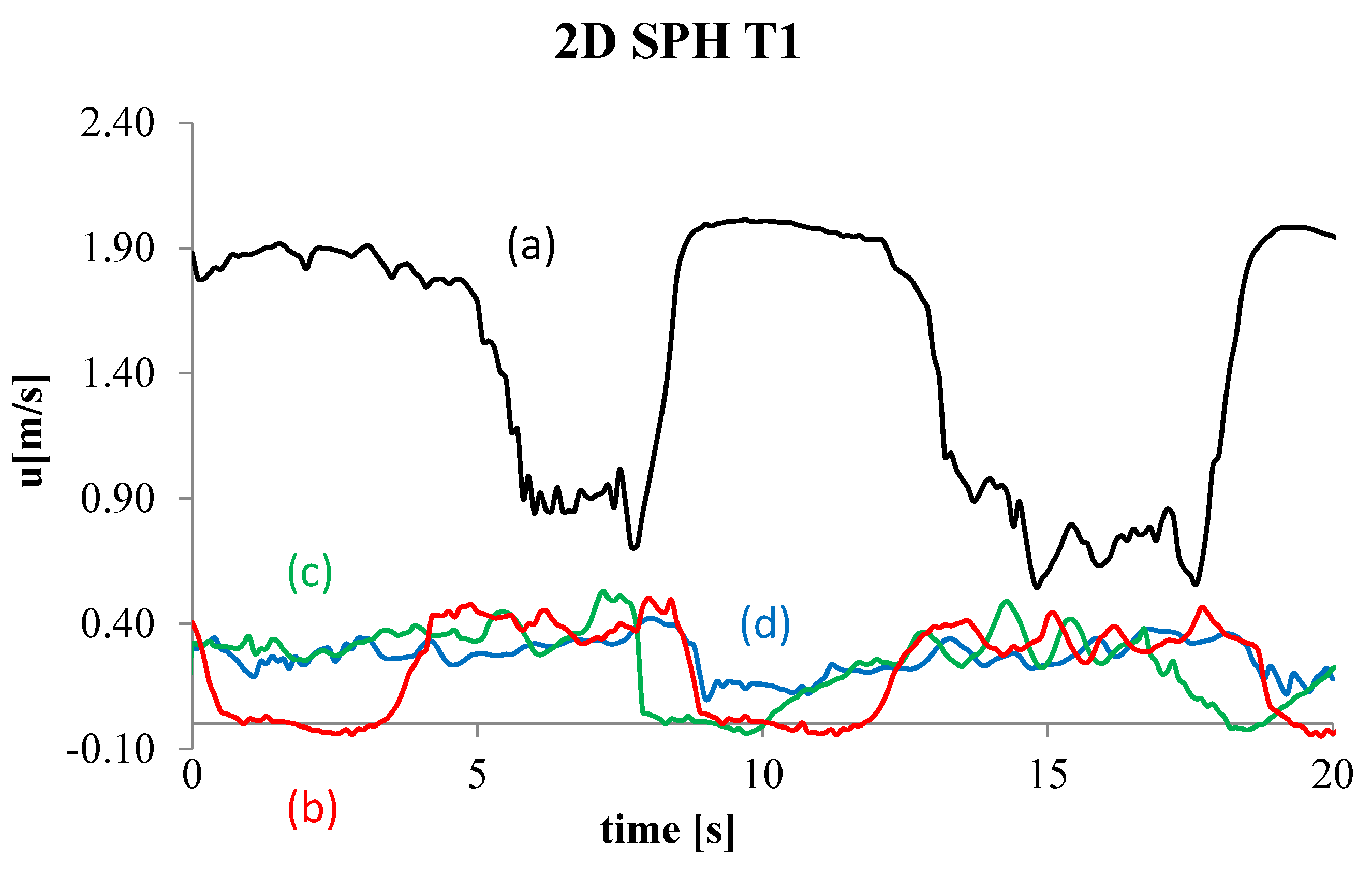
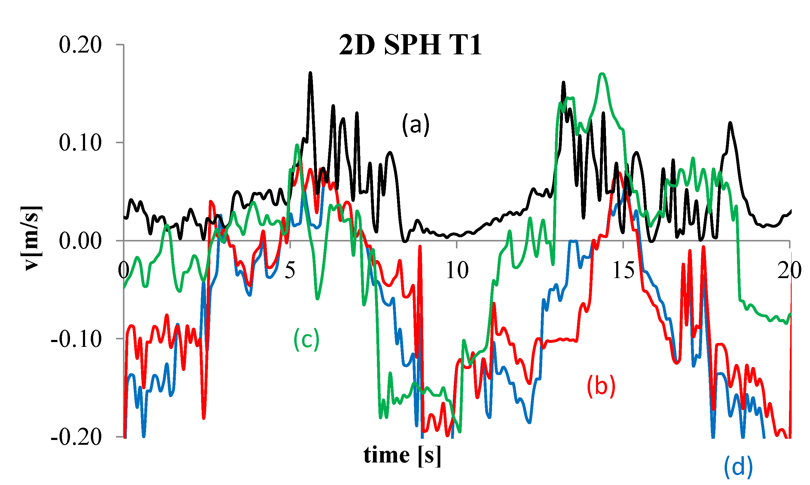
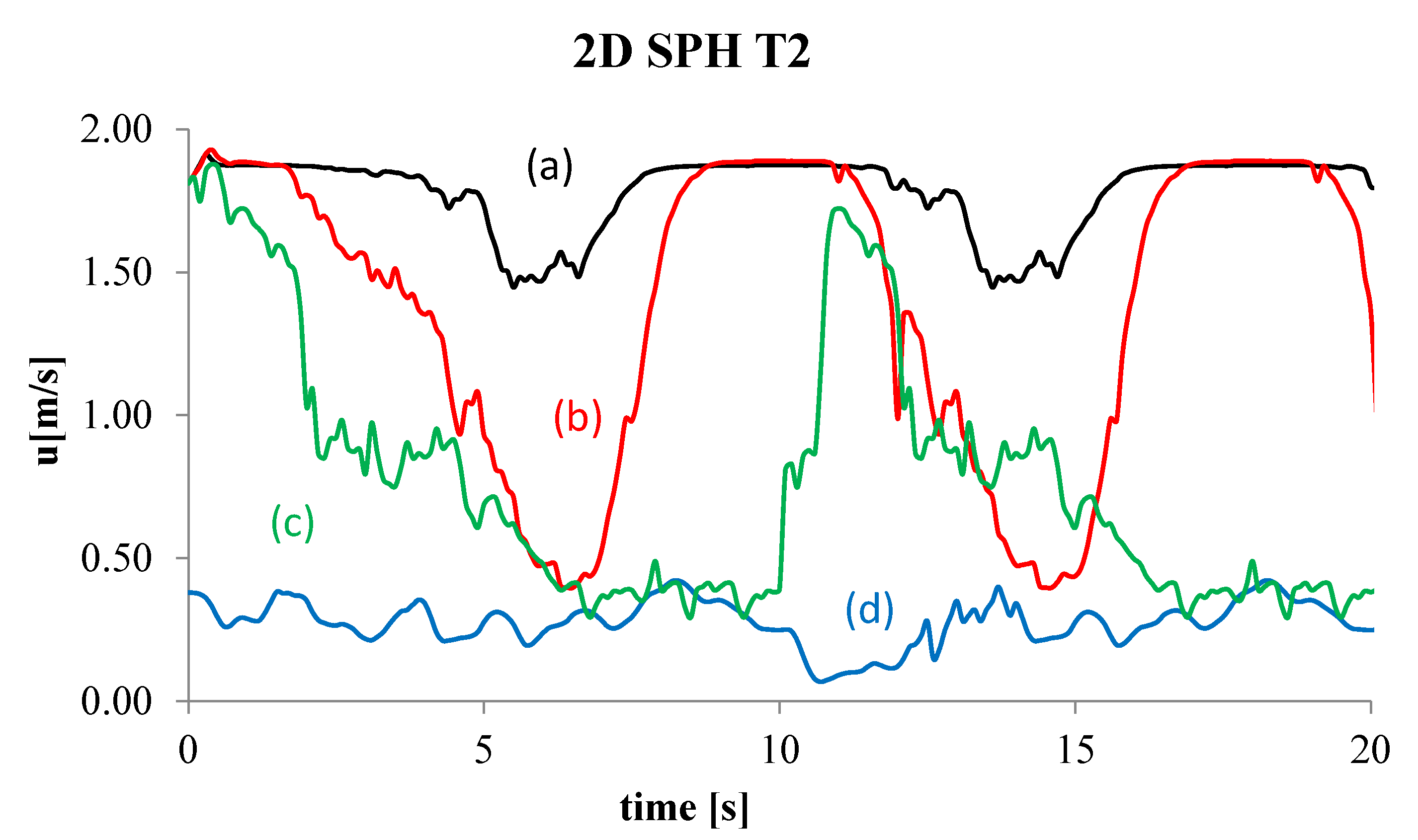
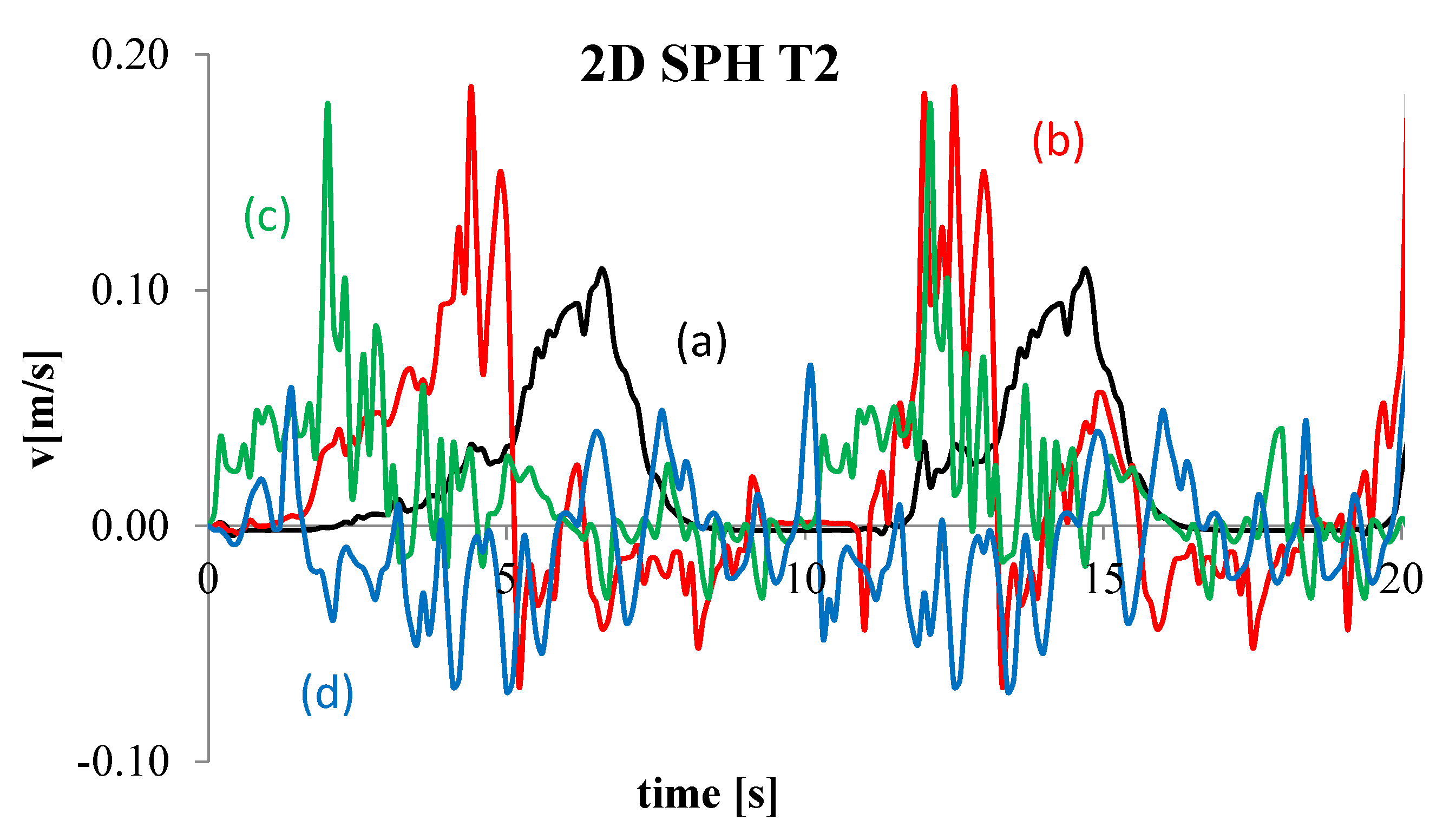
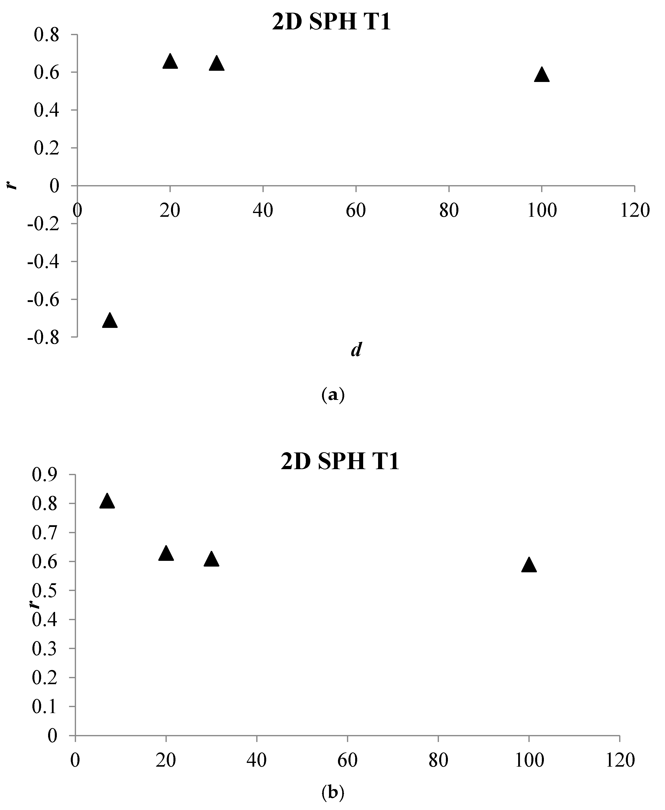
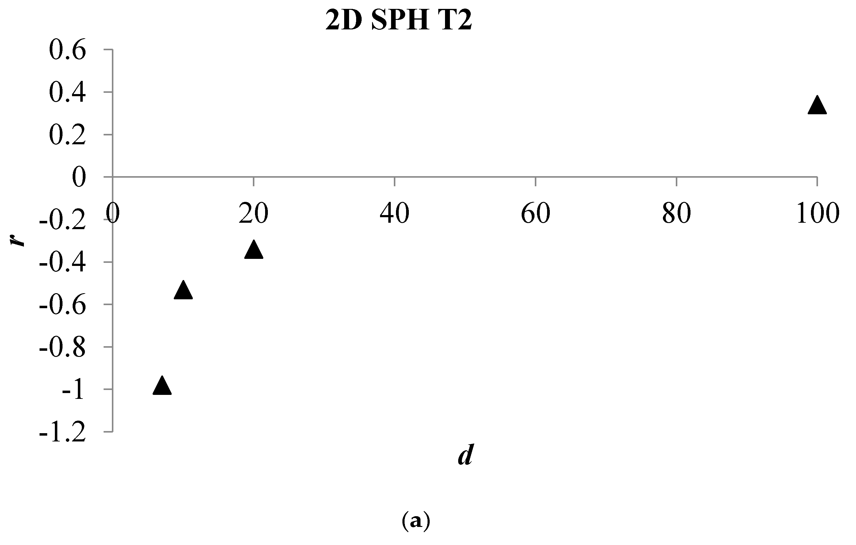
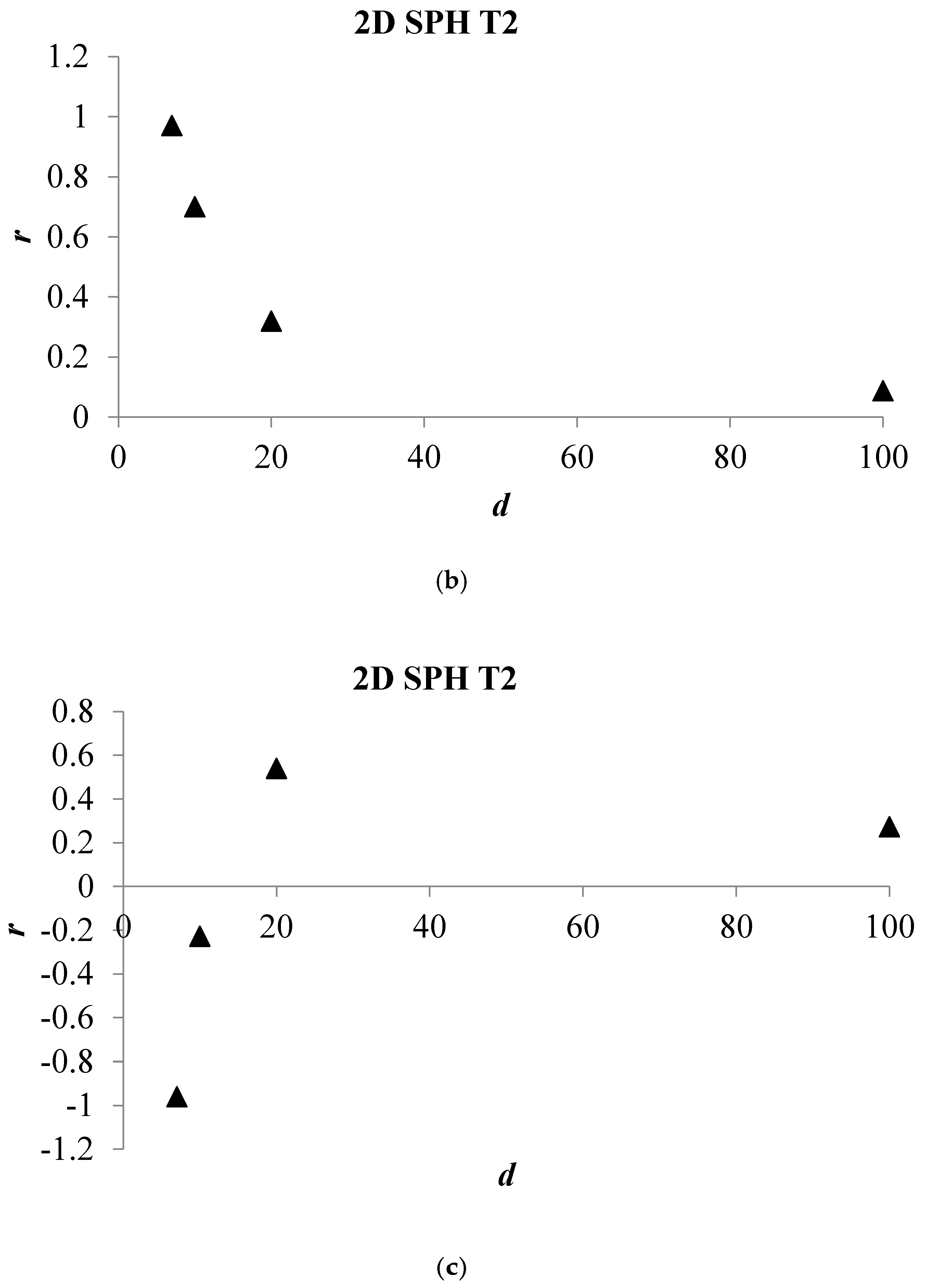
4. Numerical Tests and Results
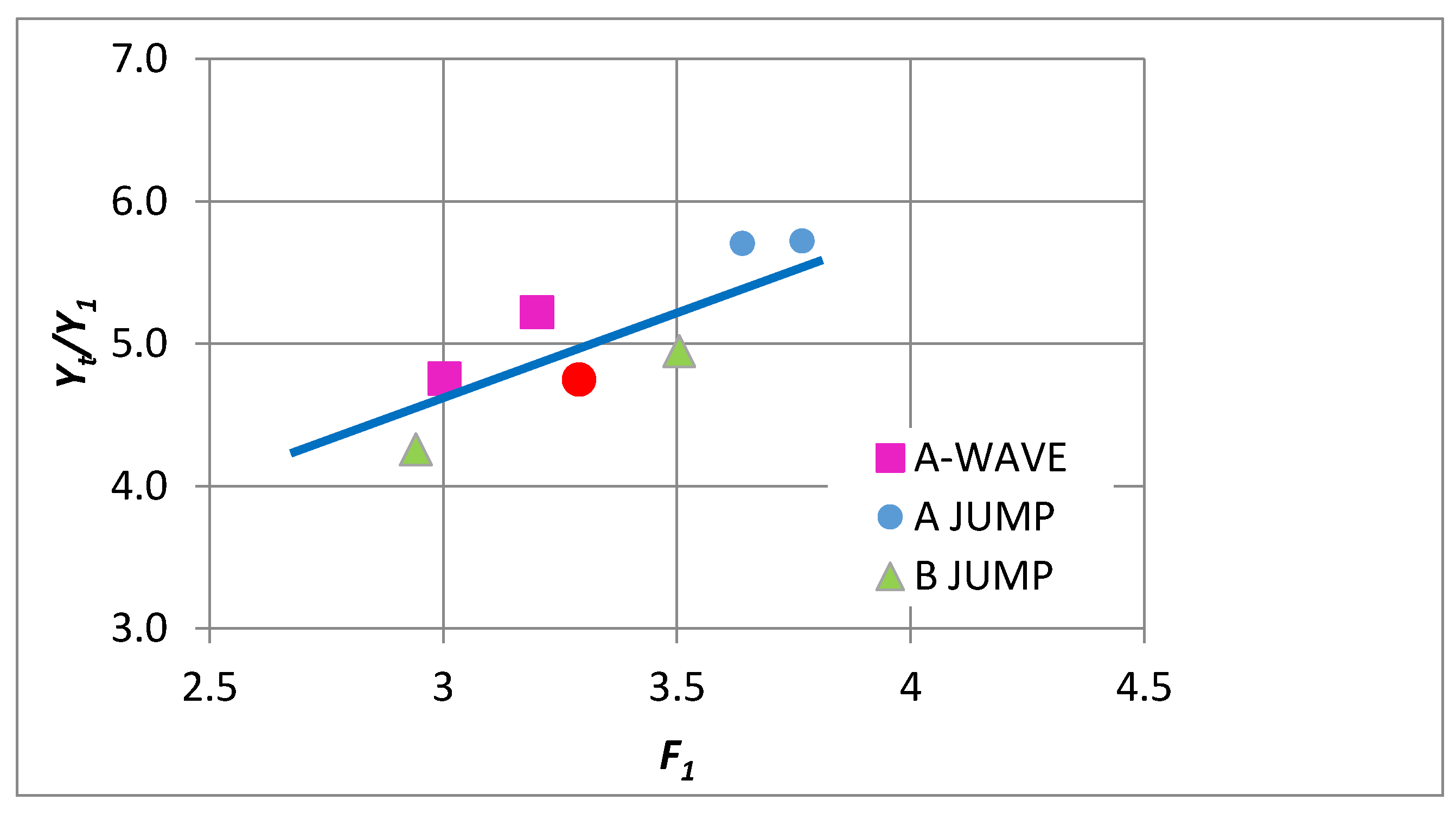
Analysis of Stable vs. Oscillating Flow Behaviour
5. Conclusions
Author Contributions
Conflicts of Interest
References
- Chow, V.T. Open Channel Hydraulics; McGraw-Hill: New York, NY, USA, 1959. [Google Scholar]
- Rajaratnam, N.; Subramanya, K. Flow equation for the sluice gate. J. Irrig. Drain. Eng. 1967, 93, 167–186. [Google Scholar]
- Moore, W.L.; Morgan, C.W. Hydraulic jump at an abrupt drop. Trans. ASCE 1959, 124, 507–524. [Google Scholar]
- Hager, W.H.; Kawagoshi, N. Hydraulic jumps at rounded drop. Proc. Instit. Civil Eng. 1990, 89, 443–470. [Google Scholar] [CrossRef]
- Ohtsu, I.; Yasuda, Y. Transition from supercritical to subcritical flow at an abrupt drop. J. Hydraul. Res. 1991, 29, 309–328. [Google Scholar] [CrossRef]
- Chanson, H.; Toombes, L. Supercritical flowat an abrupt drop: Flow patterns and aeration. Can. J. Civil. Eng. 1998, 25, 956–966. [Google Scholar] [CrossRef]
- Nebbia, G. Su taluni fenomeni alternativi in correnti libere. L’Energia Elettrica, Fasc. I 1942, XIX, 1–10. Available online: http://www.diia.unina.it/pdf/pubb0034.pdf (accessed on 12 October 2017).
- Hager, W.H.; Bretz, N.V. Hydraulic jumps at positive and negative steps. J. Hydraul. Res. 1986, 24, 237–252. [Google Scholar] [CrossRef]
- Abdel Ghafar, A.; Mossa, M.; Petrillo, A. Scour from flowdownstream of a sluice gate after a horizontal apron. In Proceedings of the Sixth International Symposium on River Sedimentation—Management of Sediment—Philosophy, Aims, and Techniques, New Delhi, India, 7–11 November 1995; Varma, C.V.J., Rao, A.R.G., Eds.; Oxford & IBH Publishing Co. Pvt. Ltd.: Delhi, India, 1995; pp. 1069–1088. [Google Scholar]
- Mossa, M.; Petrillo, A. Sui fenomeni alternativi in un risalto idraulico. In Proceedings of the Congress ‘Giornate di Studio in onore del Prof. Edoardo Orabona nel centenario della nascita’, Editoriale BIOS, Rome, Italy, 13‒14 October 1997; pp. 125–153. (In Italian). [Google Scholar]
- Mossa, M.; Tolve, U. Flow visualization in bubbly two-phase hydraulic jump. J. Fluids Eng. 1998, 120, 160–165. [Google Scholar] [CrossRef]
- Mossa, M. On the oscillating characteristics of hydraulic jumps. J. Hydraul. Res. 1999, 37, 541–558. [Google Scholar] [CrossRef]
- Wang, H.; Chanson, H. Experimental study of turbulent fluctuations in hydraulic jumps. J. Hydraul. Eng. 2015, 141, 04015010-1–04015010-10. [Google Scholar] [CrossRef]
- Wang, H.; Murzyn, F.; Chanson, H. Total pressure fluctuations and two-phase flow turbulence in hydraulic jumps. Exp. Fluids 2014, 55. [Google Scholar] [CrossRef]
- Long, D.; Rajaratnam, N.; Steffler, P.M.; Smy, P.R. Structure of flow in hydraulic jumps. J. Hydraul. Res. 1991, 29, 207–218. [Google Scholar] [CrossRef]
- Mossa, M.; Petrillo, A.; Chanson, H. Tailwater Level Effects on Flow Conditions at an Abrupt Drop. J. Hydraul. Res. 2003, 41, 39–51. [Google Scholar] [CrossRef]
- Chippada, S.; Ramaswamy, B.; Wheeler, M.F. Numerical simulation of hydraulic jump. Int. J. Num. Meth. Eng. 1994, 37, 1381–1397. [Google Scholar] [CrossRef]
- Ma, F.; Hou, Y.; Prinos, P. Numerical calculation of submerged hydraulic jumps. J. Hydraul. Res. 2001, 39, 493–503. [Google Scholar] [CrossRef]
- Carvalho, R.; Lemos, C.; Ramos, C. Numerical computation of the flow in hydraulic jump stilling basins. J. Hydraul. Res. 2008, 46, 739–752. [Google Scholar] [CrossRef]
- Meireles, I.C.; Bombardelli, F.A.; Matos, J. Air entrainment onset in skimming flows on steep stepped spillways: An analysis. J. Hydraul. Res. 2014, 52, 375–385. [Google Scholar] [CrossRef]
- Chanson, H.; Carvalho, R. Hydraulic jumps and stilling basins. Chapter 4. In Energy Dissipation in Hydraulic Structures; Chanson, H., Ed.; CRC Press, Taylor & Francis Group: Boca Raton, FL, USA, 2015; A. Balkema Book. [Google Scholar]
- Bayon, A.; Valero, D.; García-Bartual, R.; Jos, F.; Valles-MorF, J.; Lopez-Jim, P. Performance assessment of OpenFOAM and FLOW-3D in the numerical modeling of a low Reynolds number hydraulic jump. Environ. Model. Softw. 2016, 80, 322–335. [Google Scholar] [CrossRef]
- Dalrymple, R.A.; Rogers, B.D. Numerical modelling of waves with the SPH method. Coast. Eng. 2006, 53, 131–147. [Google Scholar] [CrossRef]
- De Padova, D.; Dalrymple, R.A.; Mossa, M. Analysis of the artificial viscosity in the smoothed particle hydrodynamics modelling of regular waves. J. Hydraul. Res. 2014, 52, 836–848. [Google Scholar] [CrossRef]
- Altomare, C.; Suzuki, T.; Domínguez, J.M.; Crespo, A.J.C.; Gómez-Gesteira, M.; Caceres, I. A hybrid numerical model for coastal engineering problems. In Proceedings of the 34th International Conference on Coastal Engineering (ICCE), Seoul, Korea, 15–20 June 2014. [Google Scholar] [CrossRef]
- Lind, S.J.; Stansby, P.K.; Rogers, B.D.; Lloyd, P.M. Numerical predictions of water-air wave slam using incompressible-compressible smoothed particle hydrodynamics. Appl. Ocean Res. 2015, 49, 57–71. [Google Scholar] [CrossRef]
- Ni, X.; Feng, W.B.; Wu, D. Numerical simulations of wave interactions with vertical wave barriers using the SPH method. Int. J. Numer. Methods Fluids 2014, 76, 223–245. [Google Scholar] [CrossRef]
- Shadloo, M.S.; Weiss, R.; Yildiz, M.; Dalrymple, R.A. Numerical simulation of long wave runup for breaking and nonbreaking waves. Int. J. Offshore Polar Eng. 2015, 25, 1–7. [Google Scholar]
- De Padova, D.; Mossa, M.; Sibilla, S. SPH numerical investigation of the velocity field and vorticity generation within a hydrofoil-induced spilling breaker. Environ. Fluid Mech. 2016, 16, 267–287. [Google Scholar] [CrossRef]
- Fourtakas, G.; Rogers, B.D.; Laurence, D.R. Modelling sediment resuspension in industrial tanks using SPH. La Houille Blanche 2014, 18, 39–45. (In French) [Google Scholar] [CrossRef]
- Manenti, S.; Sibilla, S.; Gallati, M.; Agate, G.; Guandalini, R. SPH simulation of sediment flushing induced by a rapid water flow. J. Hydraul. Eng. 2012, 138, 272–284. [Google Scholar] [CrossRef]
- Manenti, S.; Pierobon, E.; Gallati, G.; Sibilla, S.; D’Alpaos, L.; Macchi, E.G.; Todeschini, S. Vajont disaster: Smoothed Particle Hydrodynamics modeling of the post-event 2D experiments. J. Hydraul. Eng. 2016, 142, 1–11. [Google Scholar] [CrossRef]
- Mokos, A.; Rogers, B.D.; Stansby, P.K. Multiphase SPH modelling of violent hydrodynamics on GPUs. Comput. Phys. Commun. 2015, 196, 304–316. [Google Scholar] [CrossRef]
- Ulrich, C.; Leonardi, M.; Rung, T. Multi-physics SPH simulation of complex marine-engineering hydrodynamic problems. Ocean Eng. 2013, 64, 109–121. [Google Scholar] [CrossRef]
- Shadloo, M.S.; Oger, G.; Le Touzé, D. Smoothed particle hydrodynamics method for fluid flows, towards industrial applications: Motivations, current state, and challenges. Comput. Fluids 2016, 136, 11–34. [Google Scholar] [CrossRef]
- Ataie-Ashtiani, B.; Shobeyri, G. Numerical simulation of landslide impulsive waves by incompressible smoothed particle hydrodynamics. Int. J. Numer. Methods Fluids 2008, 56, 209–232. [Google Scholar] [CrossRef]
- Capone, T.; Panizzo, A.; Monaghan, J.J. SPH modelling of water waves generated by submarine landslides. J. Hydraul. Res. 2010, 48, 80–84. [Google Scholar] [CrossRef]
- Cartwright, B.K.; Chhor, A.; Groenenboom, P. Numerical simulation of a helicopter ditching with emergency flotation devices. In Proceedings of the 5th Spheric International workshop, Manchester, UK, 23–25 June 2010; pp. 98–105. [Google Scholar]
- Marrone, S.; Bouscasse, B.; Colagrossi, A.; Antuono, M. Study of ship wave breaking patterns using 3D parallel SPH simulations. Comput. Fluids 2012, 69, 54–66. [Google Scholar] [CrossRef]
- Zhang, A.; Cao, X.-Y.; Ming, F.; Zhang, Z.-F. Investigation on a damaged ship model sinking into water based on three dimensional SPH method. Appl. Ocean Res. 2013, 42, 24–31. [Google Scholar] [CrossRef]
- Espa, P.; Sibilla, S.; Gallati, M. SPH simulations of a vertical 2-D liquid jet introduced from the bottom of a free-surface rectangular tank. Adv. Appl. Fluid Mech. 2008, 3, 105–140. [Google Scholar]
- López, D.; Marivela, R.; Garrote, L. Smoothed Particle Hydrodynamics Model Applied to Hydraulic Structures: A Hydraulic Jump Test Case. J. Hydraul. Res. 2010, 48, 142–158. [Google Scholar] [CrossRef]
- Jonsson, P.; Jonsén, P.; Andreasson, P.; Lundström, T.; Hellström, J. Smoothed Particle Hydrodynamic Modelling of Hydraulic Jumps: Bulk Parameters and Free Surface Fluctuations. Engineering 2016, 8, 386–402. [Google Scholar] [CrossRef]
- Federico, I.; Marrone, S.; Colagrossi, A.; Aristodemo, F.; Antuono, M. Simulating 2D open-channel flows through an SPH model. Eur. J. Mech. B/Fluids 2012, 34, 35–46. [Google Scholar] [CrossRef]
- Chern, M.-J.; Syamsuri, S. Effect of Corrugated Bed on Hydraulic Jump Characteristic Using SPH Method. J. Hydraul. Eng. 2013, 139, 221–232. [Google Scholar] [CrossRef]
- De Padova, D.; Mossa, M.; Sibilla, S.; Torti, E. 3D SPH modelling of hydraulic jump in a very large channel. J. Hydraul. Res. 2013, 51, 158–173. [Google Scholar] [CrossRef]
- Ben Meftah, M.; De Serio, F.; Mossa, M.; Pollio, A. Analysis of the velocity field in a large rectangular channel with lateral shockwave. Environ. Fluid Mech. 2007, 7, 519–536. [Google Scholar] [CrossRef]
- Ben Meftah, M.; De Serio, F.; Mossa, M.; Pollio, A. Experimental study of recirculating flows generated by lateral shock waves in very large channels. Environ. Fluid Mech. 2008, 8, 215–238. [Google Scholar] [CrossRef]
- Ben Meftah, M.; Mossa, M.; Pollio, A. Considerations on shock wave/boundary layer interaction in undular hydraulic jumps in horizontal channels with a very high aspect ratio. Eur. J. Mech. B/Fluids 2010, 29, 415–429. [Google Scholar] [CrossRef]
- Mossa, M. Discussion on Relation of surface roller eddy formation and surface fluctuation in hydraulic jumps by K.M. Mok. J. Hydraul. Res. 2005, 43, 588–592. [Google Scholar] [CrossRef]
- Mossa, M.; Petrillo, A.; Chanson, H. Discussion on the “Tailwater Level Effects on Flow Conditions at an Abrupt Drop”. Unpublished work. 2004. [Google Scholar]
- Mossa, M. Experimental study of the flow field with spilling type breaking. J. Hydraul. Res. 2008, 46, 81–86. [Google Scholar] [CrossRef]
- Gomez-Gesteira, M.; Rogers, B.D.; Darlymple, R.A.; Crespo, A.J.C. State-of-the-art of classical SPH for free-surface flows. J. Hydraul. Res. 2010, 48, 6–27. [Google Scholar] [CrossRef]
- Liu, G.R.; Liu, M.B. Smoothed Particle Hydrodynamics—A Meshfree Particle Methods; World Scientific Publishing: 5 Toh Tuck Link, Singapore, 2007. [Google Scholar]
- Monaghan, J.J. Smoothed particle hydrodynamics. Annu. Rev. Astron. Astrophys. 1992, 30, 543–574. [Google Scholar] [CrossRef]
- Monaghan, J.J. Smoothed particle hydrodynamics. Rep. Progress Phys. 2005, 68, 1703–1759. [Google Scholar] [CrossRef]
- Violeau, D. Fluid mechanics and the SPH method: Theory and applications; Oxford University Press: Oxford, UK, 2012. [Google Scholar]
- Monaghan, J.J. Simulating free surface flows with SPH. J. Comput. Phys. 1992, 110, 399–406. [Google Scholar] [CrossRef]
- Wendland, H. Piecewise polynomial, positive definite and compactly supported radial functions of minimal degree. Adv. Comput. Math. 1995, 4, 389–396. [Google Scholar] [CrossRef]
- Sibilla, S. An algorithm to improve consistency in Smoothed Particle Hydrodynamics. Comput. Fluids 2015, 118, 148–158. [Google Scholar] [CrossRef]
- Lind, S.; Xu, R.; Stansby, P.; Rogers, B.; Lloyd, P.M. Incompressible smoothed particle hydrodynamics for free-surface flows: A generalised diffusion based algorithm for stability and validations for impulsive flows and propagating waves. J. Comput. Phys. 2012, 231, 1499–1523. [Google Scholar] [CrossRef]
- Khayyer, A.; Gotoh, H.; Shimizu, Y. Comparative study on accuracy and conservation properties of two particle regularization schemes and proposal of an optimized particle shifting scheme in ISPH context. J. Comput. Phys. 2017, 332, 236–256. [Google Scholar] [CrossRef]
- Vacondio, R.; Rogers, B.; Stansby, P.; Mignosa, P. Variable resolution for SPH in three dimensions: Towards optimal splitting and coalescing for dynamic adaptivity. Comput. Methods. Appl. Mech. Eng. 2016, 300, 442–460. [Google Scholar] [CrossRef]
- Sun, P.; Colagrossi, A.; Marrone, S.; Zhang, A. The δ+-SPH model: Simple procedures for a further improvement of the SPH scheme. Comput. Methods Appl. Mech. Eng. 2017, 315, 25–49. [Google Scholar] [CrossRef]
- Antuono, M.; Colagrossi, A.; Marrone, S.; Molteni, D. Free-surface flows solved by means of SPH schemes with numerical diffusive terms. Comput. Phys. Commun. 2010, 181, 532–549. [Google Scholar] [CrossRef]
- Antuono, M.; Colagrossi, A.; Marrone, S. Numerical diffusive terms in weakly-compressible SPH schemes. Comput. Phys. Commun. 2012, 183, 2570–2580. [Google Scholar] [CrossRef]
- Meringolo, D.D.; Colagrossi, A.; Marrone, S.; Aristodemo, F. On the filtering of acoustic components in weakly-compressible SPH simulations. J. Fluids Struct. 2017, 70, 1–23. [Google Scholar] [CrossRef]
- Aristodemo, F.; Tripepi, G.; Meringolo, D.D.; Veltri, P. Solitary wave-induced forces on horizontal circular cylinders: Laboratory experiments and SPH simulations. Coast. Eng. 2017, 129, 17–35. [Google Scholar] [CrossRef]
- Kazemi, E.; Nichols, A.; Tait, S.; Shao, S. SPH modelling of depth-limited turbulent open channel flows over rough boundaries. Int. J. Numer. Methods Fluids 2017, 83, 3–27. [Google Scholar] [CrossRef] [PubMed]
- Launder, B.E.; Spalding, D.B. The numerical computation of turbulent flows. Comput. Methods Appl. Meth. Eng. 1974, 3, 269–289. [Google Scholar] [CrossRef]
- Violeau, D.; Issa, R. Numerical modelling of complex turbulent free-surface flows with the SPH method: An overview. Int. J. Numer. Methods Fluids 2007, 53, 277–304. [Google Scholar] [CrossRef]
- Randles, P.W.; Libersky, L.D. Smoothed particle hydrodynamics: Some recent improvements and applications. Comput. Methods Appl. Mech. Eng. 1996, 139, 375–408. [Google Scholar] [CrossRef]
- De Padova, D.; Dalrymple, R.A.; Mossa, M.; Petrillo, A.F. An analysis of SPH smoothing function modelling a regular breaking wave. In Proceedings of the International Conference XXXI Convegno Nazionale di Idraulica e Costruzioni Idrauliche, Perugia, Italy, 9–12 September 2008; p. 182. [Google Scholar]
- Guza, R.T.; Thornton, E.B. Local and shoaled comparisons of sea surface elevations, pressures and velocities. J. Geoph. Res. 1980, 85, 1524–1530. [Google Scholar] [CrossRef]
- Petrillo, A. Evoluzione delle onde di mare su bassi fondali sabbiosi con pendenza variabile. In Proceedings of the IX Congresso Nazionale AIMET A, Bari, Italy, 7–8 Ottobre 1988. [Google Scholar]


| TEST | Run no. (Mossa 2002) | y1 (cm) | yt (cm) | V1 (m/s) | Vt (m/s) | F1 | y1/yt | Re | s (cm) | s/y1 | Jump Type |
|---|---|---|---|---|---|---|---|---|---|---|---|
| T1 | B32 | 3.5 | 16.63 | 1.93 | 0.41 | 3.3 | 4.75 | 6.10 × 10⁴ | 3.2 | 0.9 | B-wave |
| T2 | B37 | 3.7 | 17.65 | 1.81 | 0.38 | 3 | 4.76 | 5.80 × 10⁴ | 3.2 | 0.9 | A-wave |
| T3 | B38 | 3.48 | 1818 | 1.87 | 0.36 | 3.2 | 5.22 | 5.90 × 10⁴ | 3.2 | 0.9 | A-wave |
| T4 | B39 | 3.14 | 17.97 | 2.09 | 0.36 | 3.8 | 5.72 | 5.70 × 10⁴ | 3.2 | 0.9 | A-jump |
| T5 | B30 | 3.19 | 18.2 | 2.04 | 0.36 | 3.6 | 5.71 | 5.90 × 10⁴ | 3.2 | 0.9 | A-jump |
| T6 | B28 | 3.78 | 16.1 | 1.79 | 0.42 | 2.8 | 4.26 | 6.10 × 10⁴ | 3.2 | 0.9 | B-jump (Max.plung.condit.) |
| T7 | B30 | 3.39 | 16.78 | 2.02 | 0.41 | 3.5 | 4.95 | 6.00 × 10⁴ | 3.2 | 0.9 | B-jump (Max.plung.condit.) |
| TEST | Turbulence Model | η/Σ | NP |
|---|---|---|---|
| T1a | mixing-length model | 1.5 | 3000 |
| T1b | k-ε turbulence model | 1.5 | 3000 |
© 2017 by the authors. Licensee MDPI, Basel, Switzerland. This article is an open access article distributed under the terms and conditions of the Creative Commons Attribution (CC BY) license (http://creativecommons.org/licenses/by/4.0/).
Share and Cite
De Padova, D.; Mossa, M.; Sibilla, S. SPH Modelling of Hydraulic Jump Oscillations at an Abrupt Drop. Water 2017, 9, 790. https://doi.org/10.3390/w9100790
De Padova D, Mossa M, Sibilla S. SPH Modelling of Hydraulic Jump Oscillations at an Abrupt Drop. Water. 2017; 9(10):790. https://doi.org/10.3390/w9100790
Chicago/Turabian StyleDe Padova, Diana, Michele Mossa, and Stefano Sibilla. 2017. "SPH Modelling of Hydraulic Jump Oscillations at an Abrupt Drop" Water 9, no. 10: 790. https://doi.org/10.3390/w9100790
APA StyleDe Padova, D., Mossa, M., & Sibilla, S. (2017). SPH Modelling of Hydraulic Jump Oscillations at an Abrupt Drop. Water, 9(10), 790. https://doi.org/10.3390/w9100790