Article

Streamflow and Sediment Yield Prediction for Watershed Prioritization in the Upper Blue Nile River Basin, Ethiopia

1
Australian Rivers Institute and School of Engineering, Griffith University, Nathan, Queensland 4111, Australia
2
Ethiopian Ministry of Water Resources, Addis Ababa 1000, Ethiopia
3
School of Geography, the University of Melbourne, Parkville 3010, Australia
4
Blackland Research & Extension Center, Texas A&M AgriLife Research, 720 East Blackland Rd, Temple, TX 76502, USA
*
Author to whom correspondence should be addressed.
Water 2017, 9(10), 782; https://doi.org/10.3390/w9100782
Submission received: 6 August 2017 / Revised: 25 September 2017 / Accepted: 2 October 2017 / Published: 12 October 2017

Abstract

:
Inappropriate use of land and poor ecosystem management have accelerated land degradation and reduced the storage capacity of reservoirs. To mitigate the effect of the increased sediment yield, it is important to identify erosion-prone areas in a 287 km2 catchment in Ethiopia. The objectives of this study were to: (1) assess the spatial variability of sediment yield; (2) quantify the amount of sediment delivered into the reservoir; and (3) prioritize sub-catchments for watershed management using the Soil and Water Assessment Tool (SWAT). The SWAT model was calibrated and validated using SUFI-2, GLUE, ParaSol, and PSO SWAT-CUP optimization algorithms. For most of the SWAT-CUP simulations, the observed and simulated river discharge were not significantly different at the 95% level of confidence (95PPU), and sources of uncertainties were captured by bracketing more than 70% of the observed data. This catchment prioritization study indicated that more than 85% of the sediment was sourced from lowland areas (slope range: 0–8%) and the variation in sediment yield was more sensitive to the land use and soil type prevailing in the area regardless of the terrain slope. Contrary to the perception of the upland as an important source of sediment, the lowland in fact was the most important source of sediment and should be the focus area for improved land management practice to reduce sediment delivery into storage reservoirs. The research also showed that lowland erosion-prone areas are typified by extensive agriculture, which causes significant modification of the landscape. Tillage practice changes the infiltration and runoff characteristics of the land surface and interaction of shallow groundwater table and saturation excess runoff, which in turn affects the delivery of water and sediment to the reservoir and catchment evapotranspiration.

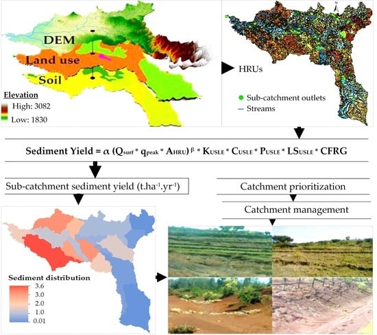
Graphical Abstract

1. Introduction

The Ethiopian Highlands, here defined as an area extending from about 1000 m above mean sea level (amsl) up to the highest peak in Ethiopia, Mount Ras Dashen (4533 m amsl), cover over half of the country and are home to the majority of the country’s population. More than 90% of the Highlands were once forested; today the percentage of forest cover is less than 4% [1]. This extensive deforestation has led to severe soil erosion and increased land degradation throughout the Ethiopian Highlands.
Excessive soil erosion in the mountainous Ethiopian Highlands has brought about reduced soil fertility and caused sedimentation in lakes and water storage reservoirs. Soil erosion and sedimentation processes have affected the whole upper Blue Nile in general [2] and the Koga catchment in particular. The Koga dam reservoir is one of the seriously affected reservoirs in the Blue Nile Basin. Most of the contributing sub-catchments are highly erodible, resulting in plenty of coarse sediments deposited in the reservoir. Since impoundment in 2008, the reservoir storage capacity has been substantially reduced because of siltation. The reduction in the flow velocity due to impoundment is a cause for deposition of sediments and a rapid decrease in the reservoir storage capacity [3,4]. This, in turn, is reducing the operational value and the life span of both the reservoir and irrigation canals.
The high soil erosion rate in the Ethiopian Highlands resulted from erosive rains, steep slopes due to the rapid tectonic uplift during the Pliocene and Pleistocene, and human impact through deforestation, overgrazing, and agricultural production [5,6,7]. In addition, the soil erosion complies with the density of forest cover in the cultivated lands to reduce the impact of high-intensity rainfall with high runoff potential [8,9,10]. Past studies from experimental small (1 km2) to large catchments (98–82,350 km2) indicated the spatial variability and temporal dynamics of sediment yield in the Ethiopian highlands (Table 1).
Sediment supply in a catchment is heterogeneous in space and time [20], depending on the land use, vegetation cover, climate, and landscape characteristics: soil type, topography, slope, and drainage conditions [21]. The Ethiopian highlands are noted for their dynamic variation in sediment yield. The spatial variation in erosion rates and total sediment yield within the Blue Nile and Atbara River systems have shown the presence of considerable spatial variability in specific sediment yield (erosion rate per unit area) ranging between 4 and 4935 t km−2 yr−1 [22]. Studies have shown how this variation in the specific sediment yield can be explained by surface vegetation cover, the mean annual rainfall, air temperature, and livestock density [22,23]. With a top-down approach [24], (i.e., generalization achieved by fingering down into the smaller-scale processes from above, catchment scale), the sediment yield in the Koga catchment (a tributary of the Blue Nile Basin) varies spatially with land cover, soil type, terrain characteristics, and climate variability. Hence, estimation of the total amount of sediment yield delivered to the Koga dam reservoir and identification of the source area of the coarse sediments that are likely to be trapped in the reservoir are critical steps in developing mitigation strategies to increase the operating life span of the reservoir.
There are a number of empirical, conceptual, and physical models to simulate catchment soil erosion. Selecting the right hydrological model for a specific catchment has always been a challenge, and field testing of watersheds and previous applicability of the model in hydrologically similar catchments could help researchers to use the proper model for their purposes. Most physical models [25] generally require hydro-meteorological, soil, topographical, and land use data as input. Besides these data, models such as APEX, EPIC, SWAT, and TOPOG [25,26] also require crop management data. Erosion modeling is even more difficult in data-scarce environments using models like EPIC, EUROSEM, KINEROS, OPUS, SPUR, and WEPP that require a large number of field input parameters for execution. The flow and sediment yield model applied in this study was the Soil and Water Assessment Tool (SWAT). SWAT was selected in the belief that the lumping nature, stationarity, and linearity problems of the rating curve could be avoided by replacing it by distributed and process-based runoff and sediment yield models. The model’s ability to predict catchment soil erosion and sediment yield at different scales from small, 0.15 km2 [27] to basin-scale, 491,700 km2 [28,29] studies and its ability to account for the spatial heterogeneity in different land management practices are additional benefits [25,26,30,31,32,33,34]. The calibration/uncertainty analyses procedures for SWAT are carried out in an integrated platform using the standalone SWAT-CUP program that links to SWAT's output text files set.
The main aim of this study was to estimate catchment streamflow and sediment yield for watershed prioritization and the specific objectives of the research were: (1) to simulate streamflow and sediment yield using the SWAT model and to evaluate the model performance through calibration and validation; (2) to undertake sensitivity analysis of streamflow and sediment yield with respect to model parameters; (3) to assess the spatial variability of sediment yield and identify the erosion hotspot sub-catchments; and (4) to quantify the amount of coarse sediment delivered into the reservoir from contributing sub-catchments.

2. Materials and Methods

2.1. Study Area

The Koga catchment is a tributary of the Gilgel Abay in the headwaters of the Blue Nile Basin. Within the catchment, there is a 21.5 m high and 1860 m long earth dam built to irrigate more than 7000 and 5600 hectares of land for dry and wet season irrigation, respectively. Since part of the northeast boundary of the reservoir (6 km upstream of the main dam) has a low spot, a saddle dam measuring 18.50 m in height and 1106 m in length was constructed to limit the extent of the reservoir. The storage capacity of the reservoir at full supply level (2015.25 m amsl) is 83.1 × 10⁶ m3.
The catchment is located approximately 36 km southwest of Bahir Dar, between 11°10′ to 11°32′ N and 37°04′ to 37°17′ E with an altitude range from 1830 m at the dam site to 3082 m amsl towards the headwater region of the catchment. The total drainage area of the catchment is 287 km2 and the length of Koga River before joining Gilgel Abay River (a major tributary of the Blue Nile) is 64 km. Upper Blue Nile river basin (Figure 1, top right) is one of the 12 river basins of the country with Lake Tana sub-basin as its main tributary (Figure 1, lower left). The study catchment (Figure 1, bottom right) is dominantly covered by mixed grass, marsh, and bush land units.

2.2. Input Data

The datasets on landscape attributes included land use, soil and digital elevation model, DEM (Figure 2). The data collected from the Ethiopian ministry of water and Energy (MoWE) [35] indicated that the dominant land use in the area was agricultural (72.1%) followed by pasture (21.2%) and bush land (6.7%). The majority of the area is covered with two soil types: Haplic Luvisols (48.3%) and Haplic Alisols (26.6%). The remaining soil classes (Lithic Leptosols, Eutric Vertisols, and Haplic Nitisols) covered 25.1% of the area. The catchment elevation ranges from 1830 to 3082 m amsl and majority of the area is below 15% (Figure 2, bottom left).
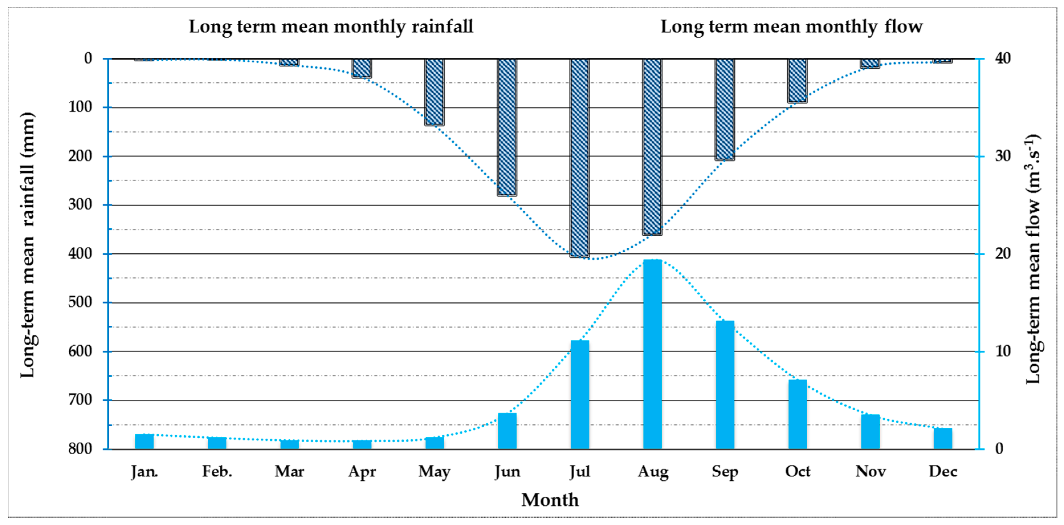
The climate of the catchment is largely controlled by distinct dry and wet seasons, receiving its moist air masses from the Indian and South Atlantic Oceans following the north–south movement of the Inter Tropical Convergence Zone [36]. The area has a unimodal rainfall pattern, with the rainy season extending from June to September, when it receives about 70 to 90% of its annual rainfall. The mean annual rainfall in the area is about 1475 mm, which varies considerably from year to year, with pronounced wetter and drier cycles [37]. The mean annual temperature of the area varies between 7 and 30 °C. The model climate data were collected from the Ethiopian National Metrological Service Agency (NMSA) [38] for a period of 19 years, 1989–2007 (Figure 3). There are two river gauges at Koga Merawi (since 1959) and the dam site (installed in 2003). The long-term (19 years) mean annual catchment discharge as obtained from MoWE [35] was 604 mm yr−1.
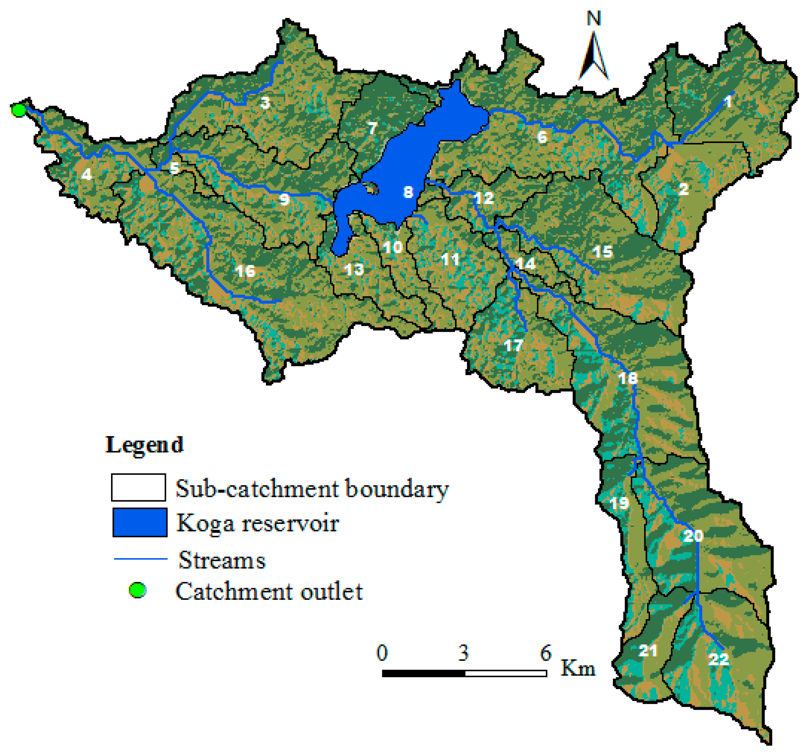
Koga dam reservoir has a dynamically varying surface area, with a maximum water level (i.e., 2015.25 m amsl) in the rainy season from May to October and the water level dropping during active irrigation periods, November to April. The reservoir extends from sub-catchment #13 in the northwest to the low area around the saddle dam in the northeast, sub-catchment 6. Sub-catchment 8 (Figure 4) is almost always completely inundated throughout the year, with only sediment loading. SWAT model-based catchment sediment yield simulation is related to the sediment resulting from erosion in the land phase portion of the model only. In this case, inundated sub-catchments (i.e., sub-catchments lying in the reservoir) have no effect on the sediment yield, but instead affect the sediment loadings from erosion in the water phase of the model.

2.3. Model Description

SWAT is a continuous time step spatially distributed hydrological model designed to simulate water, sediment, nutrient, and pesticide transport at a catchmentsscale [32,39].
The model can be divided into a number of components and modules including weather, hydrology, soil temperature and properties, bacteria and pathogens, erosion/sedimentation, nutrient, pesticide, agricultural management, plant growth, channel routing, and pond/reservoir routing components [32,40]. SWAT accounts for the impact of land management practices on streamflow, sediment discharge, and nutrient load from complex catchments with varying land use, soil, and management conditions for long periods of time [41]. SWAT, as a process-based distributed-parameter hydrological model, accounts for the spatial variability of datasets to minimize modeling errors resulting from the assumption of lumped, stationary, and linear systems.
Previous hydrological studies have also shown wide applicability of SWAT for hydro-meteorologically similar catchments and in other parts of Ethiopian basins [42,43,44,45,46,47,48].
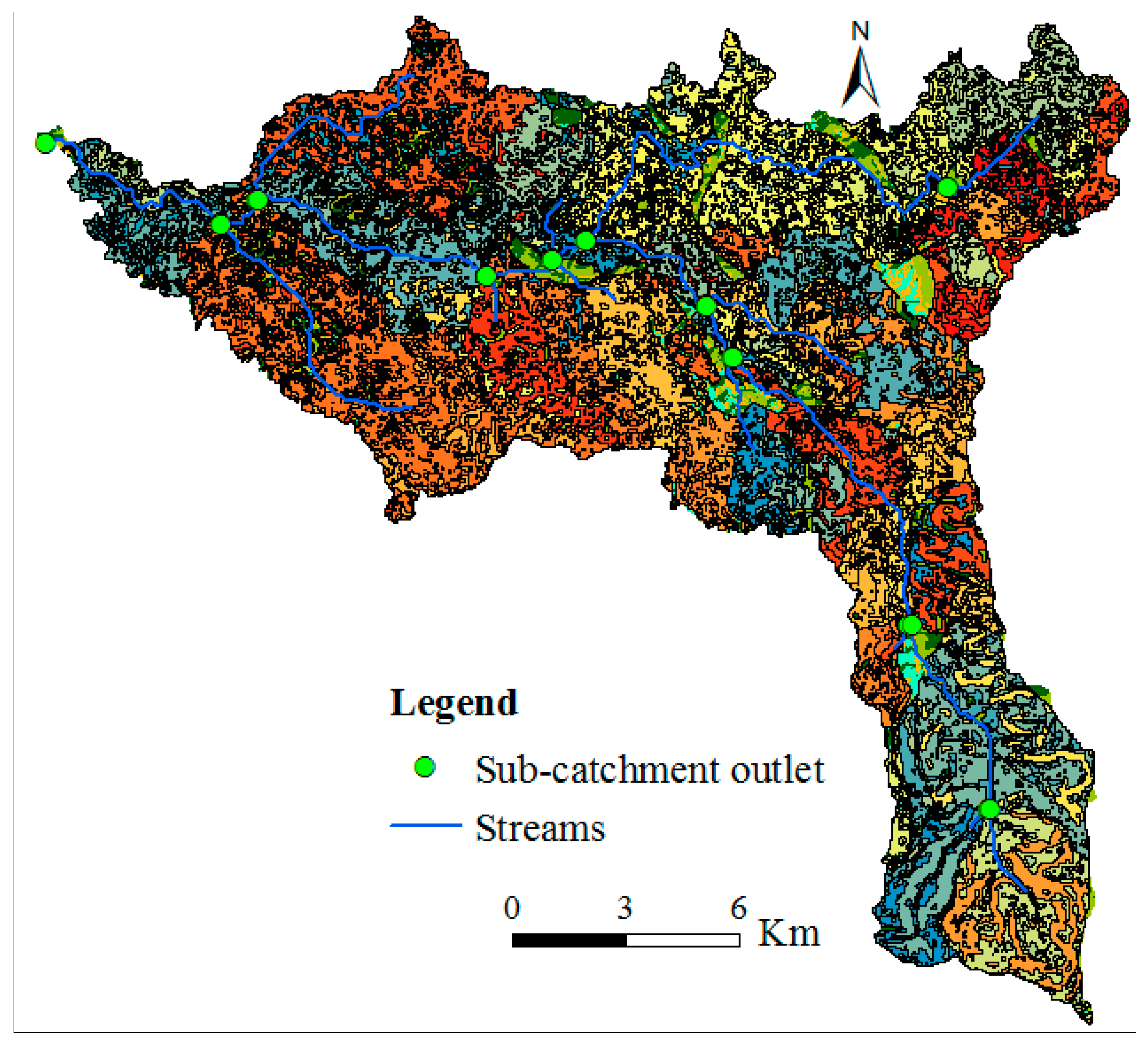
Modeling streamflow and sediment discharge at the catchment outlet involves SWAT project setup, watershed delineation, hydrological response units (HRUs) analysis, preparing and editing input tables, and model simulation. Based on the topographical characteristics of the terrain from DEM, the SWAT model describes catchment spatial variability by further splitting sub-catchments into homogeneous characteristics, lumped land areas, and smallest spatial unit (HRUs) based on topography, soil, land use, and slope [49]. The multiple land use/soil/slope method was used to define the HRU with land use (20%), soil (10%), and slope (20%) threshold [50]. The number of HRUs is defined by eliminating the percent land use, soil, and slope values that cover a percentage of the sub-catchment area less than the threshold level (Figure 5). Alternatively, a catchment can be subdivided into only sub-catchments that are characterized by dominant land use, soil type, and terrain slope.
Catchment water, sediment, and nutrient transformations and losses are predicted separately for each HRU, with predictions summed to obtain the total for each sub-catchment. Sub-catchment simulations are then routed to the associated reach and catchment outlet through the channel network [49].
Simulation of the hydrology of a watershed contains two major phases of the hydrologic cycle: the land phase and the water or routing phase. The former simulates the amount of water, sediment, nutrient, and pesticide loading carried by surface runoff from the sub-basin to the corresponding main channel. The latter controls the movement of water, sediment, nutrients, and pesticides through the channel network of the watershed [49]. Specific to the main objective of our research, the estimation of streamflow and sub-catchment sediment yield for watershed prioritization, the surface runoff and sediment yield components of the SWAT model are described. The land phase of the hydrologic cycle is simulated based on the water balance as in Equation (1):
SW t = SW 0 + i = 1 t ( R d a y Q s u r f E a W s e e p Q g w ) ,
where SWt is the final soil water content (mm), SW0 is the initial soil water content on day i (mm), t is the time (days), Rday is the amount of precipitation on day i (mm), Qsurf is the amount of surface runoff on day i (mm), Ea is the amount of evapotranspiration on day i (mm), Wseep is the amount of water entering the vadose zone from the soil profile on day i (mm), and Qgw is the amount of return flow on day i (mm).
SWAT calculates the surface erosion within each HRU using the inbuilt Modified Universal Soil Loss Equation (MUSLE). The MUSLE model [51], which is a modified version of the USLE [52], replaced the R-factor in the USLE with a term for runoff intensity to eliminate the need for a delivery ratio, improve sediment yield prediction, and allow the equation to be applied to individual storm events [41]. MUSLE estimates sediment yield from surface runoff volume, peak runoff rate, area of the HRU, soil erodibility, support practice, topographic, cover and management, and coarse fragment USLE factors. The USLE as a model estimates average annual soil loss by sheet and rill on those portions of landscape without deposition. The modified universal soil loss equation [51] is given by:
S y = α   ( Q s u r f q p e a k A H R U ) β   K U S L E C U S L E P U S L E L S U S L E C F R G ,
where Sy = HRU sediment yield (t/day); Qsurf = daily surface runoff volume (mm water/ha); qpeak = runoff peak discharge (m3 s−1); AHRU = HRU area (ha); KUSLE is the USLE soil erodibility factor (0.013 metric ton m2 h/(m3 metric ton cm), CUSLE, PUSLE, and LSUSLE are dimensionless factors accounting for HRU crop cover, soil protection, and topography as defined in the original Universal Soil Loss Equation [53,54], and CFRG is a dimensionless factor to account for coarse fragment cover (stoniness).
Williams (1975) used data collected from 18 small unequal area watersheds with considerably varying land use and collection periods for a total of 778 individual storms. To determine the most accurate prediction equation, each form of the runoff and sediment yield factors were substituted into the universal soil loss equation and evaluated by optimization [55]. The equation that best fits the data (Equation (2)) gave α and β factor values of 11.8 and 0.56, respectively. The value of the unit conversion factor α is 11.8 for metric units of the USLE soil erodibility factor, KUSLE [56,57].
However, there are changes in the spatiotemporal landscape datasets compared to the physiographic characteristics since the development of the MUSLE equation [51,58], and the modification of Williams α and β coefficients [51] in the original erosion model accounting for the possible overestimation of the MUSLE equation is state of the art [59,60]. It is also reasonable to consider current conditions of a particular catchment instead of employing the one-size-fits-all approach to modeling [61,62].
The importance of accounting for current physiographic characteristics in the MUSLE equation was supported by the developer of the MUSLE model, J.R. Williams (1975). According to Williams (1975) [51], although the runoff factor is a good sediment yield predictor, more research is needed to ensure that MUSLE is applicable for various size catchments under different agro-climatic zones. All the available watershed sediment data should also be analyzed to determine the optimum values of α and β coefficients in the prediction equation.
In addition, Madeyski and Banasik (1989) [60] verified the need to modify universal soil loss equation in their study of six small Carpathian experimental watersheds ranging in area from 32 to 77 km2. In their findings, they underlined that MUSLE with the parameters given by Williams (1975) overpredicts the observed results and thus the equation should not be transferred to other regions without prior verification.
As a result, SWAT is designed to consider these modeling gaps through an inbuilt erosion prediction algorithm that accounts for the spatial variation of the system using soil, land use, terrain, and management practice data inputs to predict catchment soil erosion and sediment yield [33,34]. In addition, the model’s ability to estimate erosion at different spatiotemporal scales, down to HRUs and small contributing sub-catchments [27], would address the default catchment geography and climate-dependent simulation errors of the original erosion prediction model, MUSLE (Equation (2)). The possible modeling errors were accounted for by calibrating the sensitive catchment flow and sediment parameters related to surface soil and cover conditions. In this phase of modeling, catchment landscape parameters were varied within the recommended range to assess the changes in the seasonal infiltration, runoff characteristics, and low and high flow and sediment extremes. The location-dependent flow and sediment-sensitive spatial parameters are grouped as soil (SOL_K.sol, SOL_AWC.sol, SOL_BD.sol); groundwater (ALPHA_BF.gw, GWQMN.gw, GW_DELAY.gw, GW_REVAP.gw, REVAPMN.gw); channelrouting (CH_EROD.rte, ALPHA_BNK.rte, CH_K2.rte, CH_N2.rte, CH_COV.rte); management (CN2.mgt, USLE_P.mgt); and Basin parameters (SPEXP.bsn and SPCON.bsn). Model sensitivity analysis is described in Section 2.3.1, Section 3.1, and Section 3.3.
Sediment transport in the channel network is a function of two simultaneous processes, deposition and degradation [49]. SWAT computes the maximum concentration of sediment in the reach at the beginning of the time step. Depending on the concentration of sediment in the reach and transport capacity of the channel, a deposition or degradation process will occur. The final amount of sediment in the reach is determined as:
S e d c h =   S e d c h , i     S e d d e e p   +   S e d d e g   ,
where Sedch is the amount of suspended sediment in the reach (metric tons), Sedch,i is the amount of suspended sediment in the reach at the beginning of the time period (metric tons), Seddep is the amount of sediment deposited in the reach segment (metric tons), and Seddeg is the amount of sediment that reenters the reach segment (metric tons). The amount of sediment transported out of the reach is calculated with Equation (4) as:
S e d o u t =   S e d c h ×   V o u t V c h   ,
where Sedout is the amount of sediment transported out of the reach (metric tons), Sedch is the amount of suspended sediment in the reach (metric tons), Vout is the volume of outflow during the time step (m3 s−1), and Vch is the volume of water in the reach segment (m3). The details of the model description can be found in the SWAT theoretical documentation [49].

2.3.1. SWAT Model Sensitivity Analysis

Sensitivity analysis describes how model output varies over a range of given input variables and is a means to accommodate a large number of parameters and multiple output variables [63]. This procedure limits the number of model parameters to the most sensitive ones that have a significant effect on calibration of hydrological models for a given catchment. The different techniques to conduct sensitivity analysis can be broadly grouped into local and global approaches [64,65]. The local technique fixes all other factors to constant nominal values while sequentially varying each of the input factors to determine the output responses. Sampling one input at a time by fixing all other inputs at constant values does not account for the interaction between inputs [66]. The global sensitivity, on the other hand, explores the entire range of input factors, and all input factors can be simultaneously varied, allowing for an investigation of output variation as a result of all inputs and their possible interaction, where output uncertainty is averaged over all input factors.
SWAT model prediction uncertainties were analyzed using SWAT-CUP programs that integrate five different optimization techniques: Sequential Uncertainty Fitting (SUFI-2) [67,68], Generalized Likelihood Uncertainty Estimation (GLUE) [69], Parameter Solution (ParaSol) [70], Particle Swarm Optimization (PSO) [71], and Markov Chain Monte Carlo (MCMC) [72,73]. We used the first four methods of optimization in this particular catchment.
The parameter sensitivities is determined by calculating the multiple regression system, which regresses the Latin hypercube “one-at-a-time” and global sensitivity generated parameters against the objective function values [74,75,76] derived by the following equation:
g   =   α + i = 1 n β i b i ,
where g is the goal function and bi is the parameter. A t-test is then used to identify the relative significance of each parameter bi. The sensitivities given by Equation (5) are estimates of the average changes in the objective function resulting from changes in each parameter, while all other parameters are changing. Thus, the global sensitivity equation gives relative sensitivities based on linear approximations and, hence, only provides partial information about the sensitivity of the objective function to model parameters. Since parameters are meant to represent the process, we thereby identified the important processes to better focus on the global sensitivity analysis in a given catchment identified by a measured data outlet [67,68,75]. However, it is apparent that the measures of sensitivity in Equation (5) are different from the sensitivities calculated in absolute sensitivity analysis, a sensitivity analysis carried out by keeping all parameters constant to realistic values, while varying each parameter within a range [68].

2.3.2. Model Prediction Uncertainty

Distributed hydrological models are designed to account for the spatial variability of climate, terrain, soil, land use, and vegetation. These watershed models are increasingly used to assess alternative strategies for improved water resources management [77,78]. However, manipulating model parameters during calibration is a challenge [79] because of overparametrization of hydrologic models [80]. Taking into account various sources of uncertainty is therefore an essential and integrated part of hydrological modeling for reliable predictions of streamflow and sediment yield.
SWAT is one of the physically-based, continuous watershed simulation models that minimize modeling errors resulting from assumption of lumped, stationary, and linear systems. Yet, the SWAT model has prediction uncertainties even if the model has been properly calibrated. This is attributed to the incomplete information on the quality and quantity of input data for model calibration, capability and appropriateness of the selected search algorithm for parameter estimation, and model structural complexity, i.e., simplifications and misrepresentation of natural catchment phenomena and processes [66,68].
In addition, SWAT uses the curve number method to estimate runoff based on the relationship between precipitation, hydrologic soil group, and land use, assuming constant parameter values throughout the catchment. However, the value and order of parameter sensitivity may vary considerably with soil, land use, and climate spatial detailing down to contributing sub-catchments for the same watershed [81].
Using SWAT’s stochastic weather generator to fill in missed weather data and improve the quality of measured flow and sediment discharge is also another source of uncertainty that may result in model over/underestimation. To minimize the effect of spatial variability in precipitation [23,48] and the possible climate input data uncertainty in extending point estimates to the whole catchment (i.e., assumption of uniform climate information), we have taken advantage of nearby multiple gauging stations in developing the climate database for SWAT.

2.3.3. Model Calibration and Validation

The SWAT model has a unique set of soil, land use, and topography parameters at HRU levels and initial estimates of parameter values from soil, land use, and other surface and subsurface process parameters were adjusted during calibration [44]. The adequacy of the SWAT model to accurately simulate streamflow and sediment yield was tested by calibrating and validating the model with streamflow and sediment data for a period of 13 calibrations (1989–2001) and six validation years (2002–2007). The first three years (1989–1991) in the flow calibration run were used for model initialization.
The time period for calibration and validation years was determined by the length of the observed data record. For sufficiently long observed data that represent different climate conditions, it is possible to split the available data equally for calibration and validation. However, when the observed record is not sufficient for equal split, the length of the data may be different in such a way that the calibration period is sufficiently long. In addition, since optimized model parameters during calibration are used for model verification without further adjustment, the data quality and information contained in the calibration data are more important than the length of the dataset considered.
Since soil erosion is directly impacted by surface runoff, the model was first calibrated for hydrology balance and streamflow, followed by sediment [32,68,82,83]. As a result, for each of the SWAT-CUP packages (SUFI-2, GLUE, ParaSol, and PSO), catchment flow parameters were first optimized and kept constant during sediment calibration. Values of flow and sediment-sensitive parameters were varied iteratively within a reasonable range for various calibration runs until a satisfactory agreement between simulated and observed datasets was achieved. The calibrated model parameters were then verified using an independent set of streamflow sediment and a sediment dataset that was not used for model calibration.
During calibration, we first fitted the average annual water balance and then the shape of the hydrograph. This was carried out in a logical order for the most sensitive parameters using SUFI-2, GLUE, ParaSol, and PSO for a combined calibration and uncertainty analysis of SWAT model.
For both calibration and validation analysis in the automatic SWAT-CUP optimization, the agreement between observed and simulated catchment streamflow and sediment data was determined using subjective and quantitative measures for recommended parameter thresholds [48,84,85]. In each of the calibration and uncertainty procedures, the final value of each model parameter that showed optimal model efficiency during calibration was used for model validation without further modification [41]. To evaluate the effect of the calibration objective function, the model was calibrated for daily and monthly flow and monthly sediment yield at the catchment outlet (sub-catchment 4).
Gauged catchment model parameters are mostly estimated by employing an ordinary least squares objective function Equation (6) and minimization of the relative error RE Equation (7). The former maximizes the Nash–Sutcliffe coefficient of efficiency by minimizing the sum of squares of errors (Equation (6)) and the later involved minimization of the relative error RE Equation (7). The least squares objective function which minimizes the sum of squares of errors is given by:
min   sum   of   squares   of   errors   =   t n [ Q m Q s ] 2 ,
where Qm and Ys are the measured and simulated flows, respectively (the difference between which is the model residual error εt). Equation (6), as an objective function, implies certain assumptions about the residuals εt [86,87]: (a) εt have zero mean and constant variance δεt (i.e., E(εt = 0), E(εt2) = δεt2; (b) the εt are independent (zero covariance).
The other objective function used in the monthly flow and sediment calibration was a minimization of the relative error RE (for minimum percent bias) between measured and simulated flow at the gauging location (sub-basin #4):
R E   =   | Q m Q s Q m | 100 % ,
where Qm and Qs are the measured and predicted monthly flow and sediment values.

2.3.4. Model Performance Evaluation

The performance of the model was evaluated to assess the correlation between simulated and observed values. Both distance and weak form-based objective functions (Table 2) were used to evaluate the performance of hydrologic models [88,89]. The performance of SWAT-CUP (calibration and uncertainty program), SUFI-2, GLUE, ParaSol, and PSO was then evaluated using objective functions; viz. P-factor (ranges between 0% and 100%), R-factor (ranges between 0 and infinity), coefficient of determination R2, Nash–Sutcliffe coefficient, NSE [90], bR2 (coefficient of determination multiplied by the coefficient of regression line), PBIAS (percent bias), KGE (Kling–Gupta efficiency) and RSR (the ratio of root mean square error (RMSE) to the standard deviation of the measured data). The first four objective functions were mainly used for both daily and monthly flow and monthly sediment calibration–validation uncertainty analysis.
The coefficient of determination, R2, is expressed as the squared ratio between the covariance and the multiplied standard deviations of the observed and predicted values. It estimates the combined dispersion against the single dispersion of the observed and predicted [96]. The range of R2 lies between 0 and 1.
R 2   =   [ i = 1 n [ ( Q m Q ¯ m ) ( Q s Q ¯ s ) ] i = 1 n ( Q m Q ¯ m ) 2 i = 1 n ( Q Y m Q ¯ s ) 2 ] 2
The Nash–Sutcliffe efficiency, NSE, proposed by Nash and Sutcliffe [90], is related to the deviation from unity of the sum of the absolute squared differences between the predicted and observed values normalized by the variance of the observed values. The normalization of the variance of the observation series results in relatively higher and lower values of NSE in catchments with higher and lower dynamics, respectively [91].
N S E   =   1     [ i = 1 n ( Q m Q s ) 2 i = 1 n ( Q m Q ¯ m ) 2 ]
where i is the time series of the measured and simulated pairs; n is the number of pairs of measured and simulated variables; m and s stand for the measured and simulated data, respectively, and the bar stands for average.
The percent difference or percent bias (PBIAS) describes the tendency of the simulated data to be greater or smaller than the observed data values over a specified period (usually the entire calibration or validation period). A value close to 0% is best, with lower values indicating satisfactory model simulation [83].
PBIAS   =   i = 1 n ( Q m Q s ) i = 1 n ( Q m ) × 100 %
RSR is the ratio of the RMSE to the standard deviation of the observations. RSR varies from 0, i.e., perfect prediction, which indicates zero residual variation, to a large positive value. In general, the lower the value of RSR, the lower the RMSE and the better the model simulation performance [83].
RSR   =   RMSE STDEV obs =   i = 1 n ( Q m Q s ) 2 i = 1 n ( Q m Q ¯ m ) 2
The Kling–Gupta efficiency, KGE, [97] is an inbuilt objective functions in the SUFI-2 and PSO SWAT-CUP programs.
KGE   =   1     ( r 1 ) 2 + ( α 1 ) 2 + ( β 1 ) 2 ,
where α = δs/δm, β = μsm and r is the linear regression coefficient between simulated and measured variable, μs and μm are means of simulated and measured data, and δs and δm are the standard deviation of simulated and measured data.
b R 2   =   Maximize :   φ = { | b | R 2   i f   | b | 1 | b | 1 R 2   i f   | b | > 1 ,
where the coefficient of determination R2 is multiplied by the coefficient of the regression line between measured and simulated data, b, [75]. This function allows for the discrepancy in magnitude of the two signals (depicted by b) as well as their dynamics (depicted by R2).

3. Results and Discussion

3.1. Parameter Sensitivity

Parameter sensitivity and ranking are measured using the t-stat value, which is the coefficient of a parameter divided by its standard error. The p-values are used to determine the significance of the sensitivity. Parameters are significant for a larger absolute t-stat and lower p-values. A larger p-value suggests that changes in the predictor values are not associated with changes in the response variable [75]. The detail of sensitivity analysis is presented in Section 2.3.1.
In this study we have evaluated the relative sensitivity values found in the parameter estimation process. The global sensitivity of parameters has been calculated using the Latin hypercube “one-at-a-time” regression systems. Table 3 illustrates the variation of ENS as a function of variation of each of the 13 most sensitive flow parameters, parameters considered for model calibration. Changes in the remaining parameter values do not cause significant changes in the model output. From Table 3, it is evident that the main sensitive streamflow parameters for the four SWAT-CUP calibration uncertainty analysis programs were initial SCS CN II value (CN2) (%), soil evaporation compensation factor (ESCO), base flow alpha factor for bank storage (ALPHA_BNK), saturated hydraulic conductivity (SOL_K), Effective hydraulic conductivity in main channel (CH_K2) [mm h−1], Moist bulk density(SOL_BD), Baseflow alpha factor (ALPHA_BF) [days], available water capacity of the layer (SOL_AWC) [mm WATER/mm soil], Treshold depth of water in the shallow aquifer required for return flow to occur (GWQMN) [mm H2O], Groundwater delay (GW_DELAY) [days], Groundwater “revap” coefficient (GW_REVAP), Threshold depth of water in the shallow aquifer for “revap” to occur (REVAPMN) [mm H2O], and Manning’s “n” value for the main channel (CH_N2). The table clearly shows differences in the rank and optimum parameter values for the four SWAT-CUP programs.
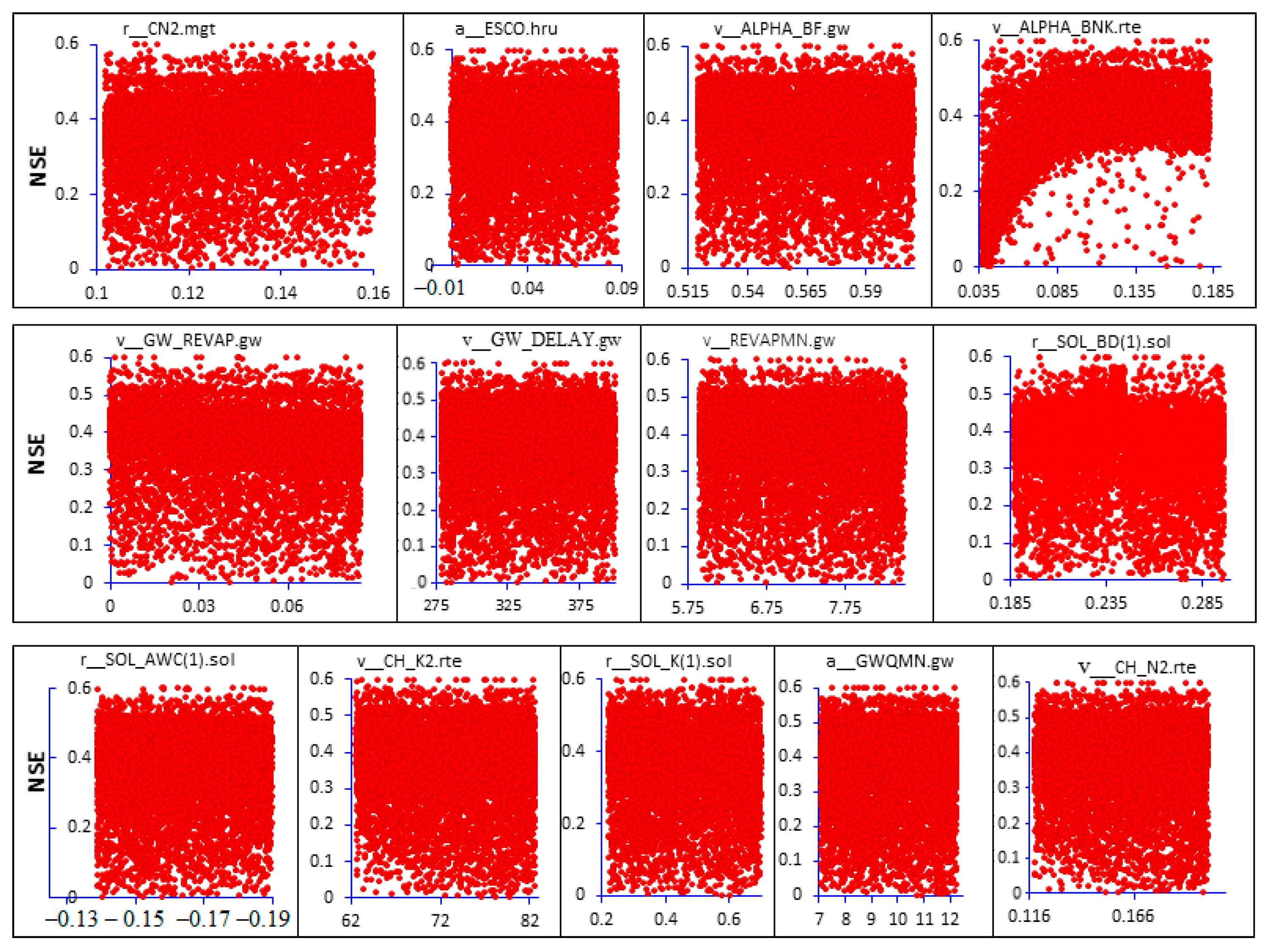
Figure 6 shows a sample dot plot based on 12,000 ParaSol simulations on a monthly basis. The relative significance of parameters is as indicated in Table 3, ranked with t-stat and p-values. The x axis shows the range of values for the sensitive flow parameters and the y axis indicates the value of the objective function, NSE.

3.2. Flow Calibration and Validation

The daily streamflow datasets used for calibration and validation of the SWAT model were obtained from the hydrology department of the Ethiopian Ministry of Water and Energy (MoWE) [2]. The hydrometric gauging station, Koga Merawi gauging station, has been in place since 1959. The station is equipped with staff gauges and an automatic water level recorder (AWLR). In this research, 19 years of continuous daily streamflow data, measured from 1989 to 2007, were used for model calibration and validation. The details of model calibration and validation are presented in Section 2.3.3.
Flow model performance rating criteria results (Table 4) showed that the agreement between measured and simulated monthly flows was indicated by NSE values of 58, 57, 58, and 59% for calibration and 58, 54, 59, and 55% for validation flows in the SWAT-CUP SUFI-2, GLUE, ParaSol, and PSO simulations. The relatively low statistical measures (NSE and R2) during the calibration and validation may have resulted from parameter and model prediction uncertainties, as explained in Section 2.3.1 and Section 2.3.2. The other source of uncertainty may be the quality of the observed streamflow data used for model calibration and validation. On the other hand, some missed climate data records were also estimated by SWAT’s stochastic weather generator. This, in turn, may result in model prediction errors.
For the purpose of determining the extent to which parameter uncertainty affects model simulation, the degree of uncertainty was quantified by a P-factor, 95PPU (95% prediction uncertainty), calculated at the 2.5% and 97.5% levels of the cumulative distribution of an output variable obtained through Latin hypercube sampling. The goodness of fit and strength of the model calibration and uncertainty procedure can also be analyzed by the R-factor, which is the relative width of 95% probability band [98].
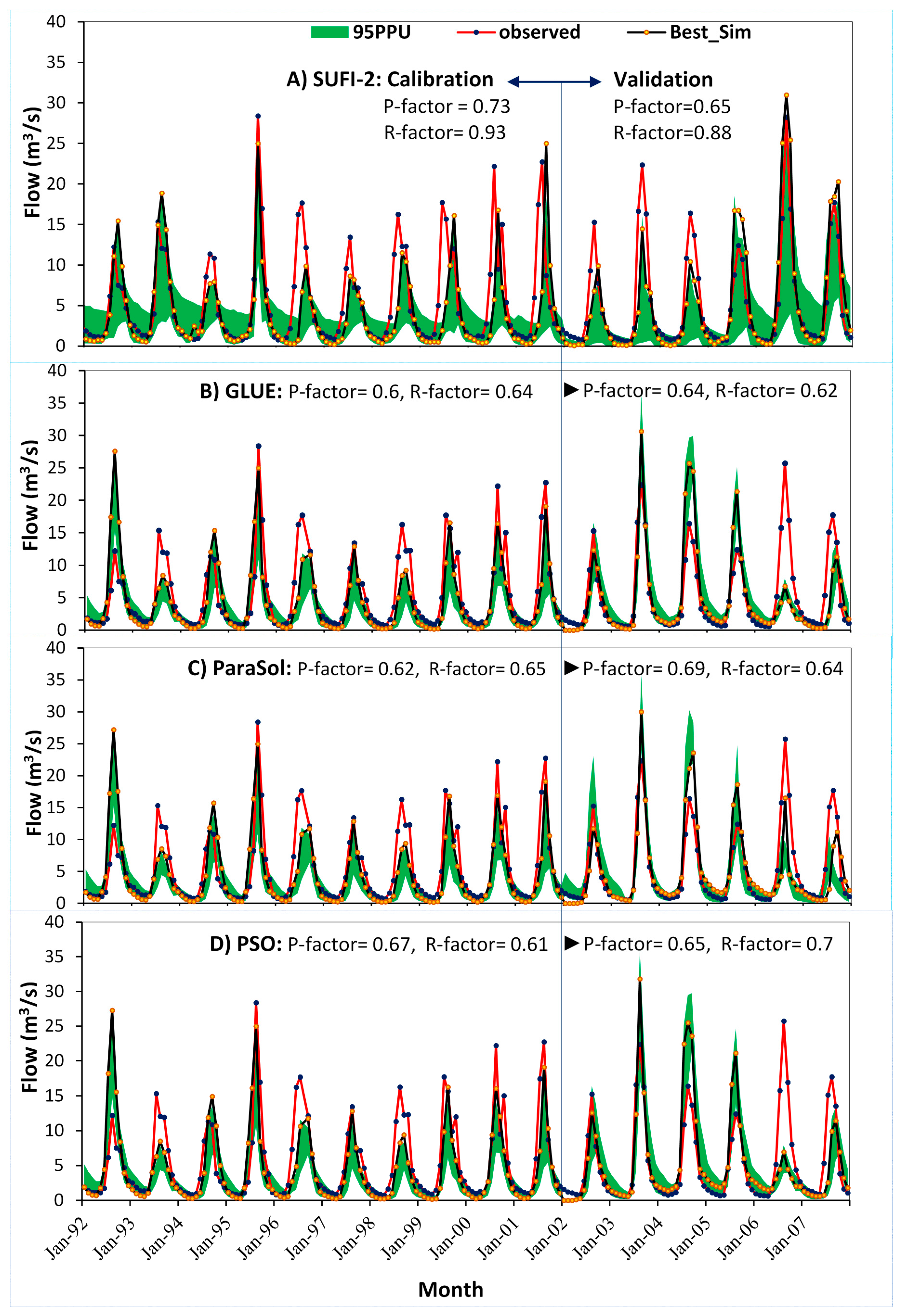
Hence, if the model captures the observed data in the 95PPU (Figure 7 and Figure 8), all uncertainties are accounted for by the parameter range. In addition, monthly predicted p values for all the SWAT-CUP simulations are considerable. For flow, a practical value of 0.6–0.8 for the P-factor and a value around 1 for the R-factor are suggested [76].
The results also showed that the model slightly underestimated flow during both calibration and validation periods, as indicated by PBIAS values (Table 4). Positive PBIAS values indicate model underestimation bias, and negative values indicate model overestimation bias [99]. This could be attributed to uncertainties related to input data quality, using the SCS curve number (CNII) method in SWAT model simulation, misrepresentation of the watershed processes, and the assumption of unique optimized parameter values throughout the catchment [68,75]. Minimizing such uncertainties could result in a well-calibrated SWAT model that can efficiently predict flows in the catchment for different management scenarios.
Figure 7 and Figure 8 show the 95PPU for calibration and validation of daily and monthly river discharge predictions, respectively. For monthly calibration and validation years, P- and R-factor values indicated a desirable certainty. For the daily simulations, however, the values of P and R are relatively low.

3.3. Sediment Yield Calibration and Validation

To determine the rate of change in model output with respect to changes in model inputs and to assess the magnitude and distribution of catchment sediment yield, initial sensitive sediment parameters were calibrated using the global sensitivity analysis procedure. Five sensitive ParaSol–SWAT–CUP sediment parameters, USLE support practice factor (v_USLE_P.mgt), Linear factor for channel sediment routing (v_SPCON.bsn), Exponential factor for channel sediment routing (v_SPEXP.bsn), Channel Erodibility factor (v_CH EROD.rte), and Channel Cover factor (v_CH COV.rte), were identified. The most sensitive parameters were calibrated with the recommended range for the whole calibration period, as indicated in Table 5.
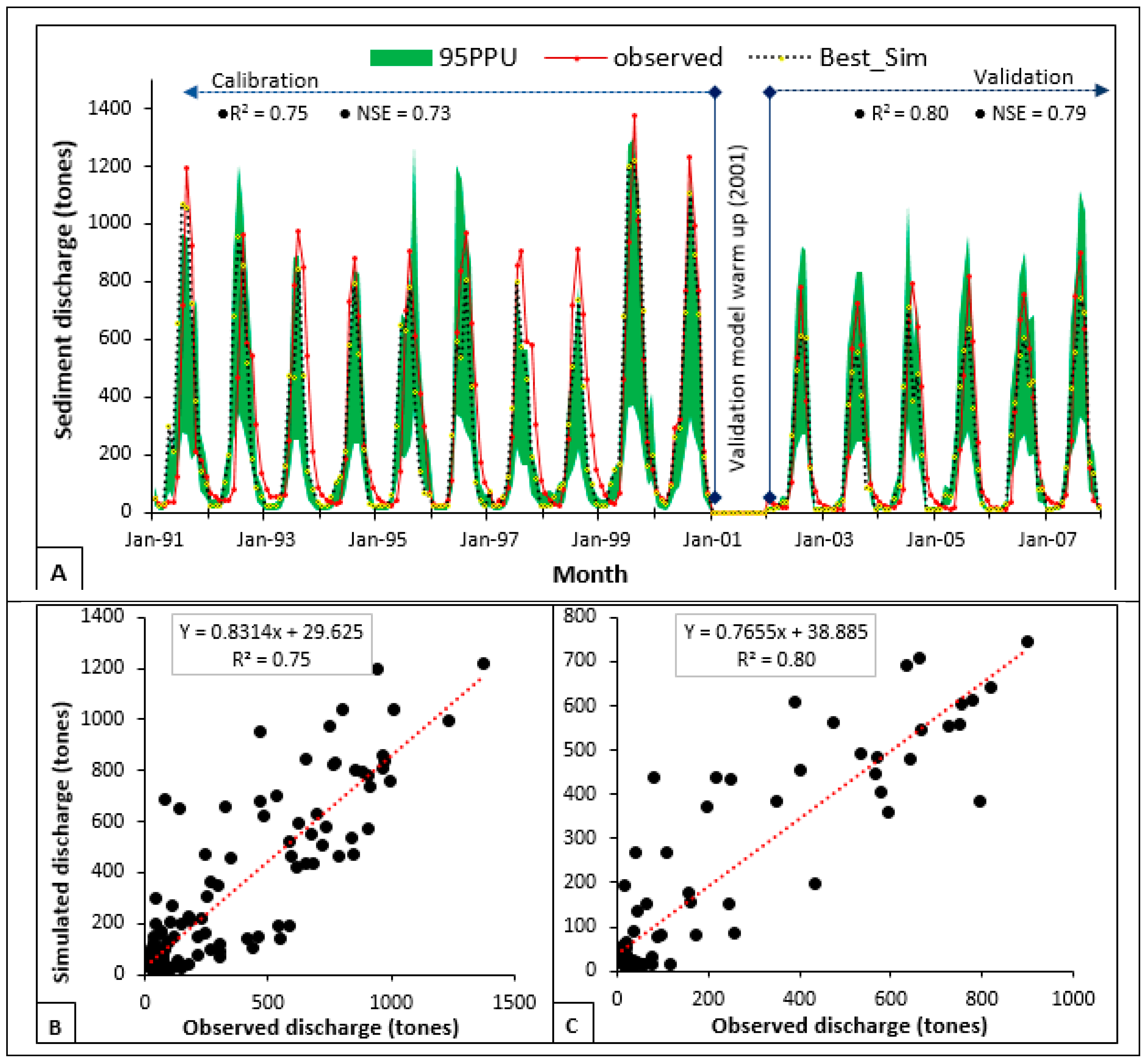
Model performance rating criteria for observed and simulated monthly average sediment yield (Table 6) indicated NSE and R2 values of 73 and 75% for calibration and 79 and 80% for validation periods, respectively. The relatively low statistical measures (NSE and R2) during model calibration may result from data quality and scarcity, streamflow processes and simulation simplifications in using observed data generated from rating curve equation (S = aQb), peak flow prediction errors, and model prediction uncertainties, as explained in Section 2.3.2.
Comparison of time-series of observed and simulated sediment yield (Figure 9) shows that the shape and timings of the peak of observed and simulated sedigraphs agree well for most of the study period. The positive PBIAS value also showed that the model slightly underestimated predicted sediment yield during both the calibration and validation periods, as indicated by PBIAS values of 7.8% and 6.4%, respectively. The results of monthly sediment calibration and validation indicate the temporal variation of outputs between the observed and simulated sediment yield.
The goodness of sediment calibration and validation uncertainty analysis can also be indicated by P-factor and R-factor, ratio of average thickness of the 95PPU band to the standard deviation of the corresponding measured variable. A P value of 64% for calibration and 67% for validation (Table 6) shows that most of the observed values were bracketed by the 95PPU; a smaller P-factor and a larger R-factor is acceptable for SWAT-CUP model sediment predictions [75]. In addition, the model prediction uncertainty is quantified by the bR2, KGE and RSR ParaSol SWAT-CUP objective function values. RSR value of 0.52 for calibration and 0.45 for validation (Table 6) shows that the ratio of root mean squared error (RMSE) to the standard deviation of the measured data, RSR, was in an acceptable range, as explained by Moriasi et al. (2007) [83].
In general, the graphical results during calibration and validation (Figure 9) indicated adequate model prediction over the range of sediment discharge. As explained in Section 2.3.4 (Table 2), the R2 [83], NSE [83,94], PBIAS [91], and RSR [83] statistical results are acceptable.

3.4. Spatial Distribution of Sediment Generation and Its Implications

3.4.1. Effect of Distributed Inputs of Soil Type and Land Use on Soil Erosion

Soil erosion is a dominant process responsible for physical degradation of the topsoil in agricultural areas. Erosion is more aggravated when the soil in the area is fertile, suitable for a wide range of agricultural uses, and susceptible to structure deterioration with tillage (e.g., Luvisols). To quantify the effects of the spatial distribution of soil type and land use on soil erosion, five main erosion source area sub-catchments (3, 7, 11, 13 and 16) covering 27.5% of the total catchment area and more than 60% of the total average annual sediment yield, were selected (Table 7).
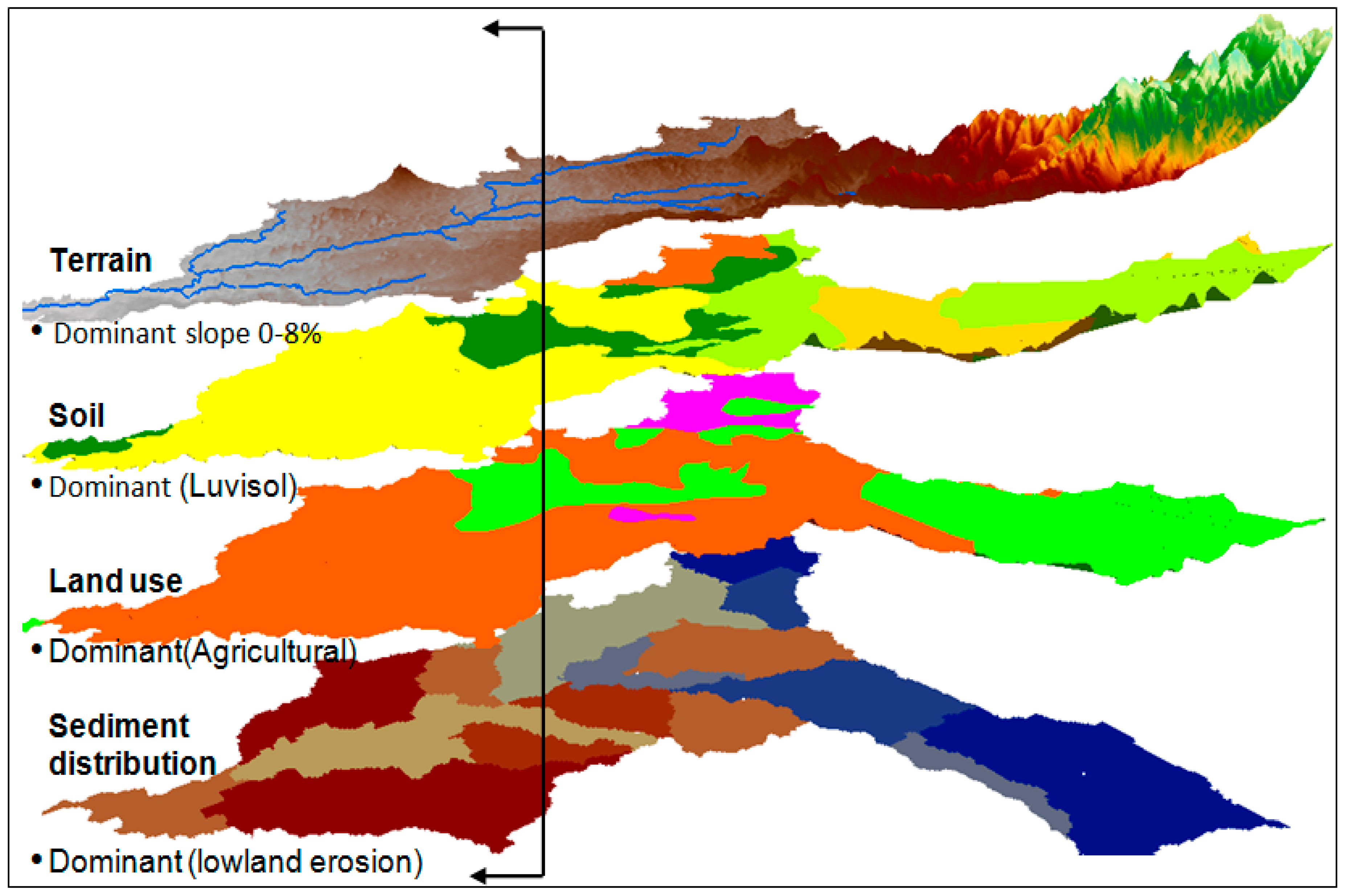
These sub-catchments were characterized by a single soil type (Luvisols) and one land use class (agricultural). In addition, the research employing catchment prioritization indicated that more than 85% of the annual average simulated suspended sediment yield was found in lowland areas (i.e., slope ranging from 0 to 8%), with one land use (agricultural) and one soil type (Luvisol). This indicates that the variation of sediment yield is more sensitive to the land use and soil type dominating the area, regardless of the terrain slope. It is also clear that lowland erosion (slope 0–8%) was more dominant than upland erosion for this particular catchment (Figure 10), which contradicts the perceived relationship between erosion and topography. The SWAT model sub-catchment sediment contribution result using the MUSLE equation and the work of Tewodros et al. (2015) [4] to identify catchment areas at risk of erosion using GIS and multi-criteria evaluation technique revealed the same dominancy of lowland erosion for the same catchment. This may result from catchment terrain slope and shallow depth ground water table in the lowland areas and near the Koga dam reservoir.
Assessing the soil formation rates of an area is vital for the evaluation of soil loss rate (the extent to which soil loss can be tolerated) and the potential of soil regeneration once soil erosion is substantially reduced. A study of soil formation rates in different agro-ecological zone of Ethiopia indicates that the range of the tolerable soil loss level for the various agro-ecological zones of Ethiopia is 2 to 18 t ha −1 yr−1 [100].

3.4.2. Sediment Source Identification

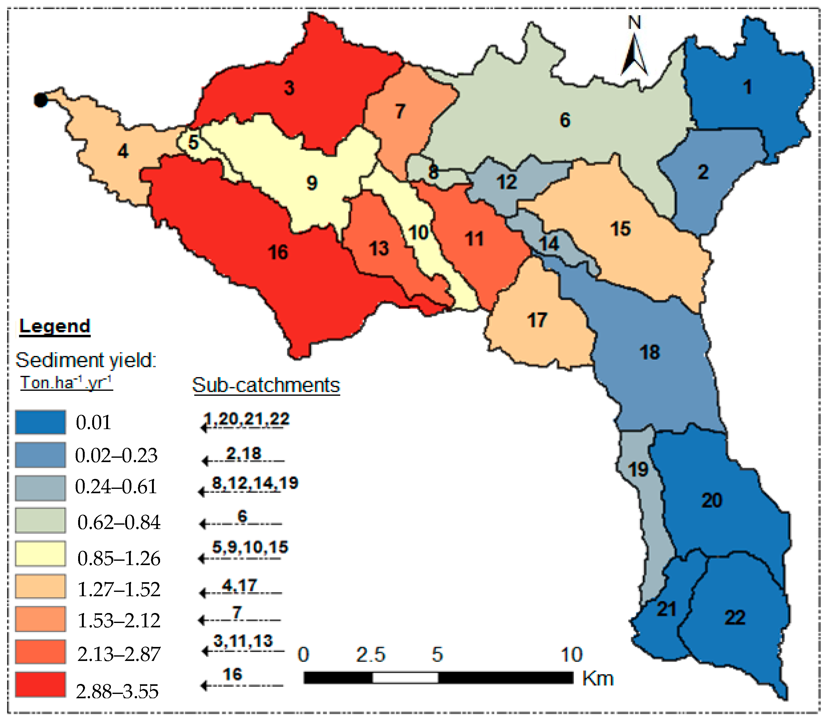
SWAT model sediment yield analysis was made to identify erosion hotspot areas and the major sources of sediment yield among the 22 contributing sub-catchments. The annual average suspended sediment yield was estimated to be 24.3 t ha−1 yr−1 and the distribution of catchment sediment yield as simulated by the model is presented in Figure 11. From the figure it can be seen that the 17 SWAT sub-catchments produced average annual sediment yields ranging from 0 to 2 t ha−1 yr−1 in high lands and 2–3.55 t ha−1 yr−1 in lowland areas. Catchment sediment yield was found to vary reasonably well with land use and soil types at each HRU.

4. Conclusions

Regardless of the SWAT model’s ability to minimize errors resulting from assumption of lumped, stationary, and linear systems, catchment modeling in a data-scarce environment is still challenging. The challenge is even greater in data-scarce regions of Africa. In addition, model structural complexity, simplifications and misrepresentation of natural catchment phenomena and processes, parameter uncertainty, and processes unknown to the modeler may result model prediction uncertainty. It is obvious that a well-calibrated SWAT model with minimal uncertainties can efficiently predict catchment runoff and sediment yield in the study area.
The calibration processes considered sensitive flow and sediment parameters to evaluate the degree of agreement between measured and simulated monthly datasets. The SWAT-CUP ParaSol model performance criteria for flow simulation resulted in (NSE = 0.58, R2 = 0.64) for calibration and (NSE = 0.59, R2 = 0.62) for validation periods, respectively. In addition, we used the 95PPU, P, and R-factors to assess the goodness of fit and strength of model calibration and uncertainty procedure. For monthly flow calibration and validation, the model captures the observed data with considerable P-factor values. The value of the R-factor was also below 1 for all SWAT-CUP programs. The agreement between observed and predicted sediment yield was indicated by NSE and R2 values of 0.73 and 0.74 for calibration and 0.79 and 0.80 for validation periods, respectively. Model sediment prediction resulted in P-factor and R-factor values of 64% and 0.75 for calibration and 67% and 0.84 for validation periods, respectively. Smaller P and larger R-factor values are also acceptable for SWAT-CUP model sediment predictions. Details of the model performance statistics for the four SWAT-CUP programs are presented in Section 3.2.
Sediment yield estimated with the SWAT model was found to correlate reasonably well with soil, land use, and topography for each HRU. The long-term (19-year) mean annual catchment discharge was 604 mm yr−1 and the model sediment yield prediction indicated an annual average catchment suspended sediment yield of 24.3 t ha−1 yr−1. As with unimodal rainfall distribution in the catchment, individual sub-catchment sediment yield and streamflow varied with the maximum value during the heavy rainfall season of the year, July to September.
In this research, attempts were made to determine the factors aggravating soil erosion and loss of storage capacity in the reservoir, to identify the potential sediment source areas for catchment prioritization and erosion control, and to provide informed estimates of the extent of sediment yield and reservoir sedimentation. Among the 22 sub-catchments, five (sub-catchments 3, 7, 11, 13, and 16) produced the highest sediment yield and are more exposed to erosion. These sub-catchments were typified by a single soil type (Luvisol) and one land use class (Agricultural). Slopes in the lowland area typically ranged from 2% to 8%. Based on this study, lowland erosion was a more important source of sediment than the upland erosion.
The research showed that lowland erosion-prone areas are typified by extensive agriculture over a single dominant soil type (Luvisols), which causes significant modification of the landscape. Tillage changes the infiltration and runoff characteristics of the land surface, which in turn affects recharge to ground water, delivery of water and sediment to the reservoir, and evapotranspiration. These processes affect the interaction of the shallow groundwater table and saturation excess runoff in lowland areas. The upland part of the watershed, on the other hand, is not a significant source of erosion due to negligible ground water saturation and minimal land disturbances.
To alleviate the alarming level of siltation in the Koga dam reservoir, we recommend the implementation of effective sub-catchment scale watershed management plans, and extensive afforestation immediately upstream of the reservoir, as well as sub-catchments that collectively contribute the majority of sediment delivery to and deposition in the reservoir. Prior to applying catchment management options, regardless of the terrain environment, the order of priority for each sub-catchment should be assessed by optimizing among the terrain, economic, labor, manmade, and natural factors.

Acknowledgments

The study was financed by Bahir Dar University–Blue Nile Water Institute under the project “Remote sensing approaches to access drought severity from multi-temporal GIMMS NDVI, rainfall and PDSI interactions for future drought monitoring”. We would like to acknowledge Blue Nile Water Institute for funding this project. Gebiaw T. Ayele would like to thank Tesfaye Shiferaw, Asegdew Gashaw, Goraw Goshu, Elias Simie, and Solomon S. Demissie. We would also like to thank MoWE and NSMA for providing the necessary data and Roderick A. Prince for editing the manuscript.

Author Contributions

All authors conceived and designed the research. Gebiaw T. Ayele expanded the text in the paper, performed flow statistical calibration–validation uncertainty analysis in SWAT-CUP, and prepared the final version of the manuscript. Engidasew Z. Teshale run ParaSol for sub-catchment sediment yield prioritization. All authors read and approved the manuscript.

Conflicts of Interest

The authors declare no conflict of interest.

References

  1. Hurni, H.; Solomon, A.; Amare, B.; Berhanu, D.; Eva, L.; Brigitte, P.; Zeleke, G. Land Degradation and Sustainable Land Management in the Highlands of Ethiopia. In Global Change and Sustainable Development: A Synthesis of Regional Experiences from Research; Hurni, H., Wiesmann, U.M., Eds.; Geographica Bernesia: Bern, Switzerland, 2010; Volume 5, pp. 187–207. [Google Scholar]
  2. Nyssen, J.; Poesen, J.; Moeyersons, J.; Haile, M.; Deckers, J.; Lang, A. Human impacts on the environment in the Ethiopian and Eritrean Highlands—A states of the art. Earth Sci. 2004, 64, 273–320. [Google Scholar] [CrossRef]
  3. Reynolds, B. Variability and Change in Koga Reservoir Volume, Blue Nile, Ethiopia. Ph.D. Thesis, Uppsala University, Uppsala, Sweden, 2013. [Google Scholar]
  4. Assefa, T.; Manoj, J.; Seifu, A.; Ephrem, Y.; Anwar, A.; Abeyou, W. Identification of Erosion Hotspot Area using GIS and MCE Technique for Koga Watershed in the upper Blue Nile Basin, Ethiopia. Am. J. Environ. Sci. 2015, 4, 245–255. [Google Scholar] [CrossRef]
  5. Ayele, G.T.; Demessie, S.S.; Mengistu, K.T.; Tilahun, S.A.; Melesse, A.M. Multitemporal land use/land cover change detection for the Batena Watershed, Rift Valley Lakes Basin, Ethiopia. In Landscape Dynamics, Soils and Hydrological Processes in Varied Climates; Melesse, A., Abtew, W., Eds.; Springer International Publishing: Cham, Switzerland, 2016; pp. 51–72. ISBN 978-3-319-18787-7. [Google Scholar]
  6. Nyssen, J.; Poesen, J.; Lanckriet, S.; Jacob, M.; Moeyersons, J.; Haile, M.; Deckers, J. Land Degradation in the Ethiopian Highlands. In Landscapes and Landforms of Ethiopia; Paolo, B., Ed.; World Geomorphological Landscapes; Springer: Dodrecht, The Netherlands, 2015; pp. 369–385. [Google Scholar]
  7. Asres, R.S.; Tilahun, S.A.; Ayele, G.T.; Melesse, A.M. Analyses of land use/land cover change dynamics in the upland watersheds of Upper Blue Nile Basin. In Landscape Dynamics, Soils and Hydrological Processes in Varied Climates; Melesse, A., Abtew, W., Eds.; Springer International Publishing: Cham, Switzerland, 2016; pp. 73–91. [Google Scholar]
  8. Guzman, C.; Tilahun, S.; Zegeye, A.; Tammo, S. Suspended sediment concentration-discharge relationships in the sub-humid Ethiopian highlands. Hydrol. Earth Syst. Sci. 2013, 17, 1067–1077. [Google Scholar] [CrossRef]
  9. Abebayehu, A.; Moges, A. Rill Erosion Assessment in Cultivated Lands and Farmers Perception on Soil Erosion, A Case of Delbo Wogene Micro-Watershed Southern Ethiopia. J. Biol. Agric. Healthc. 2015, 5, 87–115. [Google Scholar]
  10. Gelagaya, H.S.; Minale, A.S. Soil loss estimation using GIS and Remote sensing techniques: A case of Koga watershed, Northwestern Ethiopia. ISWCR 2016, 4, 126–136. [Google Scholar] [CrossRef]
  11. Hurni, H. Land degradation, famine and resource scenarios in Ethiopia. In World Soil Erosion and Conservation; David, P., Ed.; Cambridge University Press: Cambridge, UK, 1993; pp. 27–62. [Google Scholar]
  12. Tadesse, G. Land Degradation: A challenge to Ethiopia. Environ. Manag. 2001, 27, 815–826. [Google Scholar] [CrossRef]
  13. Nyssen, J.; Poesen, J.; Moeyersons, J.; Haile, M.; Josef, D. Dynamics of soil erosion rates and controlling factors in the Northern Ethiopian Highlands—Towards a sediment budget. Earth Surf. Process. Landf. 2007, 33, 695–711. [Google Scholar] [CrossRef] [Green Version]
  14. World Bank. The Cost of Land Degradation in Ethiopia: A Review of Past Studies; World Bank: Washington, DC, USA, 2007; pp. 1–21. [Google Scholar]
  15. Bewket, W.; Teferi, E. Assessment of soil erosion hazard and prioritization for treatment at the watershed level: Case study in the Chemoga watershed, Blue Nile Basin, Ethiopia. Land Degrad. Dev. 2009, 20, 609–622. [Google Scholar] [CrossRef]
  16. Abraha, A.Z. Assessment of Spatial and Temporal Variability of River Discharge, Sediment Yield and Sediment-Fixed Nutrient Export in Geba River Catchment, Northern Ethiopia; Katholieke Universiteit: Leuven, Belgium, 2009. [Google Scholar]
  17. Vanmaercke, M.; Zenebe, A.; Poesen, J.; Neyssen, J.; Verstraeten, G.; Deckers, J. Sediment dynamics and the role of flash floods in sediment export from medium-sized catchments: A case study from the semi-arid tropical highlands in northern Ethiopia. J. Soils Sediment. 2010, 10, 611–627. [Google Scholar] [CrossRef] [Green Version]
  18. Eleni, Y.; Alexander, E.; Günter, B. Temporal variation of suspended sediment transport in the Koga catchment, North Western Ethiopia and environmental implications. Hydrol. Process. 2013, 28, 5972–5984. [Google Scholar]
  19. Gizachew, A.; Yihenew, G.S. Soil loss estimation for soil conservation planning using geographic information system in Guang watershed, Blue Nile basin. J. Environ. Earth Sci. 2015, 5, 126–134. [Google Scholar]
  20. Bofu, Y.; David, N. Temporal and spatial variation of sediment yield in the Snowy Mountains region, Australia. In Variability in Stream Erosion and Sediment Transport, Proceedings of the Canberra Symposium, Canberra, Australia, 11–13 May 1994; The Australian Government Publishing Service: Canberra, Australia, 1994. [Google Scholar]
  21. Marttila, H.; Klöve, B. Dynamics of erosion and suspended sediment transport from drained peatland forestry. J. Hydrol. 2010, 388, 414–425. [Google Scholar] [CrossRef]
  22. Vincent, B.; Veerle, V.; Atkilt, G.; Jean, P.; Semunesh, G. Human impact on sediment fluxes within the Blue Nile and Atbara River basins. Geomorphology 2012, 181, 231–241. [Google Scholar]
  23. Awulachew, S.; Ahmed, A.; Haileselassie, Y.A.; Bashar, K.; McCartney, M.; Steenhuis, T. Improved Water and Land Management in the Ethiopian Highlands and Its Impact on Downstream Stake Holders Dependent on the Blue Nile; CPWF Project Report; Consultative Group on International Agricultural Research Challenge Programme on Water and Food: Montpellier, France, 2010. [Google Scholar]
  24. Klemes, V. Conceptualization and scale in hydrology. J. Hydrol. 1983, 65, 1–23. [Google Scholar] [CrossRef]
  25. Pandey, A.; Himanshu, S.K.; Mishra, S.; Singh, V.P. Physically based soil erosion and sediment yield models revisited. Catena 2016, 147, 595–620. [Google Scholar] [CrossRef]
  26. Jeong, J.; Narayanan, K.; Jeff, A.; Glick, R.; Gosselink, L.; Raghavan, S. Development and integration of sub-hourly rainfall–Runoff modeling capability within a watershed model. Water Resour. Manag. 2010, 24, 4505–4527. [Google Scholar] [CrossRef]
  27. Chanasyk, D.S.; Mapfumo, E.; Willms, W. Quantification and simulation of surface runoff from fescue grassland watersheds. Agric. Water Manag. 2003, 59, 137–153. [Google Scholar] [CrossRef]
  28. Arnold, J.G.; Muttiah, R.S.; Srinivasan, R.; Allen, P.M. Regional estimation of base flow and groundwater recharge in the upper Mississippi basin. J. Hydrol. 2000, 227, 21–40. [Google Scholar] [CrossRef]
  29. Hunink, J.; Niadas, I.; Antonaropoulos, P.; Droogers, P.; de Vente, J. Targeting of intervention areas to reduce reservoir sedimentation in the Tana catchment (Kenya) using SWAT. Hydrol. Sci. J. 2013, 58, 1–15. [Google Scholar] [CrossRef]
  30. Arnold, J.G.; Williams, J.R.; Maidment, D.R. Continuous-time water and sediment-routing model for large basins. J. Hydraul. Eng. 1995, 121, 171–183. [Google Scholar] [CrossRef]
  31. Arnold, J.G.; Srinivasan, R.; Muttiah, R.; Williams, J. Large area hydrologic modeling and assessment. Part I: Model development. J. Am. Water Resour. Assoc. 1998, 34, 73–89. [Google Scholar] [CrossRef]
  32. Arnold, J.; Kiniry, J.; Srinivasan, R.; Williams, J.; Haney, E.; Neitsch, S. Soil and Water Assessment Tool, Input/Output File Documentation; Texas Water Resources Institute: College Station, TX, USA, 2012; pp. 1–650. [Google Scholar]
  33. Bisantino, T.; Bingner, R.; Chouaib, W.; Gentile, F.; Liuzzi, G. Estimation of runoff, peak discharge and sediment load at the event scale in a medium-size Mediterranean watershed using the ANNAGNPS model. Land Degrad. Dev. 2015, 26, 340–355. [Google Scholar] [CrossRef]
  34. Taguas, E.V.; Gómez, J.A.; Mateos, P.; Denisi, L. Modelling the rainfall runoff relationships in a large olive orchard catchment in southern Spain. Water Resour. Manag. 2015, 29, 2361–2375. [Google Scholar] [CrossRef]
  35. MoWR. Spatial and Hydrological Data; Ministry of Water Resources, The Federal Democratic Republic of Ethiopia: Addis Abeba, Ethiopia, 2009.
  36. Mohamed, Y.A.; van den Hurk, B.J.; Savenije, H.H.; Bastiaanssen, W.G. Hydroclimatology of the Nile: Results from a regional climate model. Hydrol. Earth Syst. Sci. 2005, 9, 263–278. [Google Scholar] [CrossRef]
  37. Jemberie, M.A.; Awass, A.A.; Melesse, A.M.; Ayele, G.T.; Demissie, S.S. Seasonal rainfall-runoff variability analysis, lake Tana sub-basin, upper Blue Nile basin, Ethiopia. In Landscape Dynamics, Soils and Hydrological Processes in Varied Climates; Melesse, A., Abtew, W., Eds.; Springer International Publishing: Cham, Switzerland, 2016; pp. 341–363. [Google Scholar]
  38. NMSA. Metreological Data Agency; The Ethiopian National Metreological Services Agency: Addis Abeba, Ethiopia, 2009. [Google Scholar]
  39. Arnold, J.G.; Allen, P.M. Estimating hydrologic budgets for three Illinois watersheds. J. Hydrol. 1996, 176, 57–77. [Google Scholar] [CrossRef]
  40. Gassman, P.; Reyes, M.; Green, C.; Arnold, J. The soil and water assessment tool: Historical development, applications and future directions. Trans. ASABE 2007, 50, 1211–1250. [Google Scholar] [CrossRef]
  41. Neitsch, S.L.; Arnold, J.G.; Kiniry, J.R.; Williams, J.R. Soil and Water Assessment Tool (SWAT) User’s Manual; Version 2000; Grassland Soil and Water Research Laboratory: Temple, TX, USA; Texas Water Resources Institute: Collage Station, TX, USA, 2002; pp. 1–506. [Google Scholar]
  42. Welde, K. Identification and prioritization of sub-watersheds for land and water management in Tekeze dam watershed, Northern Ethiopia. ISWCR 2016, 4, 30–38. [Google Scholar]
  43. Shawul, A.; Alamirew, T.; Dinka, M. Calibration and validation of SWAT model and estimation of water balance components of Shaya mountainous watershed, Southeastern Ethiopia. Hydrol. Earth Syst. Sci. 2013, 10, 13955–13978. [Google Scholar] [CrossRef]
  44. Hassen, M.; Assen, M.; Tena, A.; Assefa, M. Modeling of sediment yield in Maybar gauged watershed using SWAT, northeast Ethiopia. Catena 2015, 127, 191–205. [Google Scholar] [CrossRef]
  45. Dile, Y.; Berndtsson, R.; Setegn, S. Hydrological Response to Climate Change for Gilgel Abay River, in the Lake Tana Basin—Upper Blue Nile Basin of Ethiopia. PLoS ONE 2013, 8, 1–13. [Google Scholar] [CrossRef] [PubMed]
  46. Seka, A.M.; Awass, A.A.; Melesse, A.M.; Ayele, G.T.; Demissie, S.S. Evaluation of the Effects of Water Harvesting on Downstream Water Availability Using SWAT. In Landscape Dynamics, Soils and Hydrological Processes in Varied Climates; Melesse, A., Abtew, W., Eds.; Springer International Publishing: Cham, Switzerland, 2016; pp. 763–787. [Google Scholar]
  47. Moges, M.; Schmitter, P.; Tilahun, S.; Langan, S.; Dagnew, D.; Akale, A.; Steenhuis, T. Suitability of Watershed Models to Predict Distributed Hydrologic Response in the Awramba Watershed in Lake Tana basin. Land Degrad. Dev. 2016, 28, 1386–1397. [Google Scholar] [CrossRef]
  48. Kaleab, H.; Michael, M.; Manoj, K. Runoff and Sediment Modeling Using SWAT in Gumera Catchment, Ethiopia. OJMH 2013, 3, 196–205. [Google Scholar] [CrossRef]
  49. Neitsch, S.L.; Arnold, J.G.; Kiniry, J.R.; Williams, J.R. Soil and Water Assessment Tool Theoretical Documentation; Version 2009; Texas Water Resources Institute: Collage Station, TX, USA, 2011; pp. 1–647. [Google Scholar]
  50. Winchell, M.; Srinivasan, R.; Di Luzio, M.; Arnod, J. Arcswat 2.3 Interface for Swat2005 User’s Guide; Texas Water Resources Institute: Collage Station, TX, USA, 2005. [Google Scholar]
  51. Williams, J. Sediment-yield prediction with universal equation using runoff energy factor. In Present and Prospective Technology for Predicting Sediment Yield and Sources; Agriculture Research Service, US Department of Agriculture: Washington, DC, USA, 1975; pp. 244–252. [Google Scholar]
  52. Wischmeier, W.H.; Smith, D.D. Predicting Rainfall Erosion from Cropland East of the Rocky Mountains-Guide for Selection of Practices for Soil and Water Conservation; US Department of Agriculture: Washington, DC, USA, 1965.
  53. Wlschmeler, W.; Smith, D. Predicting Rainfall-Erosion Losses—A Guide to Conservation Planning; US Department of Agriculture: Washington, DC, USA, 1978; Volume 537, pp. 1–60.
  54. Chad, F.; Hatim, S.; Jaehak, J. Analysis and simulation of large erosion events at central Texas unit source watersheds. J. Hydrol. 2015, 527, 494–504. [Google Scholar]
  55. Decoursey, D.G.; Snyder, W.M. Computer-oriented method of optimizing hydrologic model parameters. J. Hydrol. 1969, 9, 34–56. [Google Scholar] [CrossRef]
  56. Sadeghi, S. Application of MUSLE in prediction of sediment yield in Iranian conditions. In Proceedings of the ISCO 2004—13th International Soil Conservation Organization Conference, Brisbane, Australia, 4–8 July 2004; pp. 1–4. [Google Scholar]
  57. Cârdei, P. The Dimensional analysis of the USLE—MUSLE Soil Erosion Model. Proc. Rom. Acad. Ser. B 2010, 3, 249–253. [Google Scholar]
  58. Williams, J.R.; Berndt, H.D. Sediment yield prediction based on watershed hydrology. Trans. ASABE 1977, 20, 1100–1104. [Google Scholar] [CrossRef]
  59. Banasik, K.; Walling, D.E. Predicting Sedimentgraphs for a Small Agricultural Catchment. Nord. Hydrol. 1996, 27, 275–294. [Google Scholar]
  60. Madeyski, M.; Banasik, K. Applicability of the modified universal soil loss equation in small Carpathian watersheds. Catena 1989, 14, 75–80. [Google Scholar]
  61. Savenije, H.G. HESS Opinions “The art of hydrology”. Hydrol. Earth Syst. Sci. 2009, 13, 157–161. [Google Scholar] [CrossRef]
  62. Sadeghi, S.; Gholami, L.; Darvishan Khaledi, A.; Saeidi, P. A review of the application of the MUSLE model worldwide. Hydrol. Sci. J. 2014, 59, 365–375. [Google Scholar] [CrossRef]
  63. Van Griensven, A. Sensitivity, Auto-Calibration, Uncertainty and Model Evaluation in SWAT2005; UNESCO-IHE: Delft, The Netherlands, 2005. [Google Scholar]
  64. Saltelli, A.; Torantola, S.; Chan, K. A quantitative model-independent method for global sensitivity analysis of model output. Technometrics 1999, 41, 39–56. [Google Scholar] [CrossRef]
  65. Saltelli, A. What is sensitivity analysis. In Sensitivity Analysis; Saltelli, A., Chan, K., Scott, E., Eds.; Wiley: New York, NY, USA, 2000; p. 42. ISBN 978-0-471-99892-1. [Google Scholar]
  66. Muleta, M.; Nicklow, J. Sensitivity and uncertainty analysis coupled with automatic calibration for a distributed watershed model. J. Hydrol. 2005, 306, 127–145. [Google Scholar] [CrossRef]
  67. Abbaspour, K.C.; Johnson, A.; Van Genuchten, M.T. Estimating uncertain flow and transport parameters using a sequential uncertainty fitting procedure. Vadose Zone J. 2004, 3, 1340–1352. [Google Scholar] [CrossRef]
  68. Abbaspour, K.C.; Yang, J.; Maximov, I.; Siber, R.; Bogner, K.; Mieleitner, J.; Srinivasan, R. Modelling hydrology and water quality in the pre-alpine/alpine Thur watershed using SWAT. J. Hydrol. 2007, 333, 413–430. [Google Scholar] [CrossRef]
  69. Beven, K.; Binley, A. The future of distributed models e model calibration and uncertainty prediction. Hydrol. Process. 1992, 6, 279–298. [Google Scholar] [CrossRef]
  70. Van Griensven, A.; Meixner, T. Methods to quantify and identify the sources of uncertainty for river basin water quality models. Water Sci. Technol. 2006, 53, 51–59. [Google Scholar] [CrossRef] [PubMed]
  71. Zhang, J.; Li, Q.; Guo, B.; Gong, H. The comparative study of multi-site uncertainty evaluation method based on swat model. Hydrol. Process. 2015, 29, 2994–3009. [Google Scholar] [CrossRef]
  72. Marshall, L.; Nott, D.; Sharma, A. A comparative study of Markov chain Monte Carlo methods for conceptual rainfall-runoff modeling. Water Resour. Res. 2004, 40, 1–11. [Google Scholar] [CrossRef]
  73. Vrugt, J.; Gupta, H.; Bouten, W.; Sorooshian, S. A shuffled complex evolution Metropolis algorithm for optimization and uncertainty assessment of hydrologic model parameters. Water Resour. Res. 2003, 39, 1–14. [Google Scholar] [CrossRef]
  74. Holvoet, K.; Griensven, A.; Seuntjens, P. Sensitivity analysis for hydrology and pesticide supply towards. Phys. Chem. Earth 2003, 30, 518–526. [Google Scholar] [CrossRef]
  75. Abbaspour, K.C. SWAT-CUP: SWAT Calibration and Uncertainty Programs; Swiss Federal Institute of Aquatic Science and Technology Eawag: Duebendorf, Switzerland, 2015; pp. 1–100. [Google Scholar]
  76. Faramarzi, M.; Abbaspour, K.C.; Adamowicz, W.L.; Wei, L.; Fennell, J.; Zehnder, A.J.; Goss, G.G. Uncertainty based assessment of dynamic freshwater scarcity in semi-arid watersheds of Alberta, Canada. J. Hydrol. Reg. Stud. 2017, 9, 48–68. [Google Scholar] [CrossRef]
  77. Shi, P.; Chen, C.; Srinivasan, R.; Zhang, X.; Cai, T.; Fang, X.; Li, Q. Evaluating the SWAT model for hydrological modeling in Xixian watershed and comparison with the XAJ model. J. Am. Water Resour. Manag. 2011, 25, 2595–2612. [Google Scholar] [CrossRef]
  78. Koutalakis, P.; Zaimes, G.; Ioannou, K.; Iakovoglou, V. Application of the SWAT model on torrents of the Menoikio, Greece. Fresen. Environ. Bull. 2017, 26, 1210–1215. [Google Scholar]
  79. Abu El-Nasr, A.; Arnold, J.; Feyen, J.; Berlamont, J. Modeling the hydrology of a catchment using a distributed and a semi distributed model. Hydrol. Process. 2005, 19, 573–587. [Google Scholar] [CrossRef]
  80. Beven, K.A. Discussion of distributed hydrological modelling. In Distributed Hydrological Modelling; Abbott, M.R., Ed.; Kluwer Academic: Dordrecht, The Netherlands, 1996; pp. 255–278. [Google Scholar]
  81. Barrett, E.C. Satellite remote sensing of precipitation: Progress and problems. In Remote Sensing and Hydrology, Wallingford, United Kingdom, 2001; Owe, M., Brubaker, K., Ritchie, J., Rango, A., Eds.; International Association of Hydrological Sciences: Rennes, France, 2001. [Google Scholar]
  82. Santhi, C.; Arnold, J.G.; Williams, J.R.; Dugas, W.A.; Srinivasan, R.; Hauck, L.M. Validation of the SWAT model on a large river basin with point and nonpoint sources. J. Am. Water Resour. Assoc. 2001, 37, 1169–1188. [Google Scholar] [CrossRef]
  83. Moriasi, D.N.; Arnold, J.G.; Van Liew, M.W.; Bingner, R.L.; Harmel, R.D.; Veith, T.L. Model evaluation guidelines for systematic quantification of accuracy in watershed simulations. ASABE 2007, 50, 885–900. [Google Scholar] [CrossRef]
  84. Shimelis, G.S.; Ragahavan, S.; Assefa, M.M.; Bijan, D. SWAT model application and prediction uncertainty analysis in the Lake Tana basin, Ethiopia. Hydrol. Process. 2009, 24, 357–367. [Google Scholar]
  85. Iris, K. SWAT for Assessing Negative Impacts of Erosion in Lake Tana Basin; Technical University of Munich: Munich, Germany, 2016. [Google Scholar]
  86. Clarke, R. A review of some mathematical models used in hydrology, with observations on their calibrations and their use. J. Hydrol. 1973, 19, 1–20. [Google Scholar] [CrossRef]
  87. Xu, C.-Y. Statistical analysis of parameters and residuals of a conceptual water balance model—Methodology and case study. Water Resour. Manag. 2001, 15, 75–92. [Google Scholar] [CrossRef]
  88. Guinot, V.; Cappelaere, B.; Delenne, C.; Ruelland, D. Towards improved criteria for hydrological model calibration: Theoretical analysis of distance and weak form-based functions. J. Hydrol. 2011, 401, 1–13. [Google Scholar] [CrossRef]
  89. Bennett, N.; Croke, B.; Guariso, G.; Guillaume, J.; Hamilton, S.; Jakeman, A.; Andreassian, V. Characterizing performance of environmental models. Environ. Model. Softw. 2013, 40, 1–20. [Google Scholar] [CrossRef]
  90. Nash, J.E.; Sutcliffe, J. River flow forecasting through conceptual models: Part I. A discussion of principle. J. Hydrol. 1970, 10, 282–290. [Google Scholar] [CrossRef]
  91. Legates, D.R.; McCabe, G.J. Evaluating the use of “goodness-of-fit” measures in hydrologic and hydroclimatic model validation. Water Resour. Res. 1999, 35, 233–241. [Google Scholar] [CrossRef]
  92. Krause, P.; Boyle, D.; Bäse, F. Comparison of different efficiency criteria for hydrological model assessment. Adv. Geosci. 2005, 5, 89–97. [Google Scholar] [CrossRef]
  93. McCuen, R.H.; Knight, Z.; Cutter, A.G. Evaluation of the Nash–Sutcliffe Efficiency Index. J. Hydrol. Eng. 2006, 11, 597–602. [Google Scholar] [CrossRef]
  94. Boskidis, I.; Gikas, G.; Sylaios, G.; Tsihruntzis, V. Hydrologic and Water Quality Modeling of Lower Nestos River Basin. Water Resour. Manag. 2012, 26, 3023–3051. [Google Scholar] [CrossRef]
  95. Hogue, T.; Sorooshian, S.; Gupta, H.; Holz, A.; Braatz, D. A multistep automatic calibration scheme for river forecasting models. J. Hydrometeorol. 2000, 1, 524–542. [Google Scholar] [CrossRef]
  96. Rodgers, J.L.; Nicewander, W.A. Thirteen ways to look at the correlation coefficient. Am. Stat. 1988, 42, 59–66. [Google Scholar] [CrossRef]
  97. Gupta, H.V.; Kling, H.; Yilmaz, K.K.; Martinez, G.F. Decomposition of the mean squared error and NSE performance criteria: Implications for improving hydrological modelling. J. Hydrol. 2009, 377, 80–91. [Google Scholar] [CrossRef]
  98. Yang, J.; Abbaspour, K.C.; Reichert, P.; Yang, H. Comparing uncertainty analysis techniques for a SWAT application to Chaohe Basin in China. J. Hydrol. 2008, 358, 1–23. [Google Scholar] [CrossRef]
  99. Gupta, H.V.; Sorooshian, S.; Yapo, P.O. Status of automatic calibration for hydrologic models: Comparison with multilevel expert calibration. J. Hydrol. Eng. 1999, 4, 135–143. [Google Scholar] [CrossRef]
  100. Hurni, H. Soil Conservation Manual for Ethiopia: Field Guide for Conservation Implementation; Ministry of Agriculture: Addis Abeba, Ethiopia, 1985.
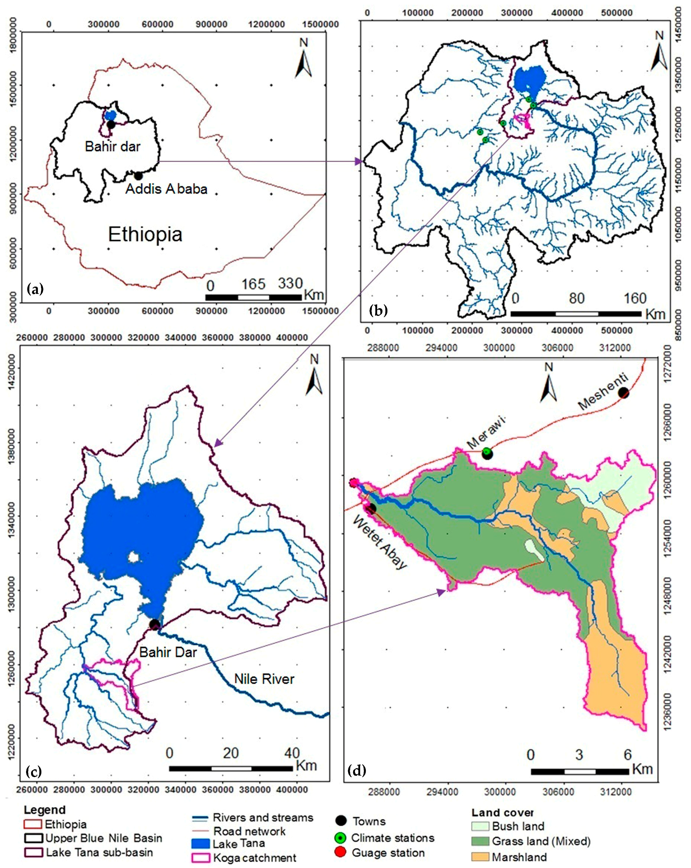
Figure 1. Location map of the study area: (a) geographical setting of the upper Blue Nile river basin in the country map; (b) network of rivers in the upper Blue Nile river basin; (c) Lake Tana sub-basin and its tributary river network; and (d) land use units in the study area.
Water 09 00782 g001
Figure 2. Koga catchment GIS data attributes: (a) soil, river network, and elevation lines; (b) land use; (c) sub-catchment boundaries and slope distribution; (d) terrain elevation map.
Water 09 00782 g002
Figure 3. Catchment long-term mean monthly rainfall and streamflow (1989–2007).
Water 09 00782 g003
Figure 4. Koga dam reservoir and the contributing sub-catchments.
Water 09 00782 g004
Figure 5. Hydrologic response unit (HRU) map.
Water 09 00782 g005
Figure 6. Dot plot of NSE coefficient against each aggregate SWAT parameters conditioning with ParaSol based on 12,000 monthly calibration streamflow simulations.
Water 09 00782 g006
Figure 7. Daily observed flow, 95% model uncertainty, and best estimates for calibration (1992–2001) and validation (2002–2007): SUFI-2 (A), GLUE (B), ParaSol (C), and PSO (D).
Water 09 00782 g007
Figure 8. Monthly observed flow, 95% model uncertainty, and best estimates for calibration (1992–2001) and validation (2002–2007): SUFI-2 (A), GLUE (B), ParaSol (C), and PSO (D).
Water 09 00782 g008
Figure 9. Monthly catchment sediment yield for calibration (1991–2000) and validation (2002–2007) (A); scatter plot of observed and simulated monthly sediment discharge (Qs) for calibration (1991–2000) (B); and validation (2002–2007) (C).
Water 09 00782 g009
Figure 10. Variation of catchment sediment yield with terrain slope and the effect of spatially heterogeneous distributed inputs of soil and land use.
Water 09 00782 g010
Figure 11. SWAT classified sub-catchments for prioritization (Sub-catchments 1–22) and distribution of SWAT simulated annual sediment yield in t ha−1 yr−1.
Water 09 00782 g011
Table 1. Soil loss estimates from different studies in the Ethiopian highlands.
ReferencesSoil Loss in t ha−1 yr−1Scale
SpatialTemporal
1[11]42Plot based on cultivated fields
2[12]31Entire highlands
3[13]14.8199 ha agriculture-dominated *
4[14]130Plot based on cultivated lands
35Entire highlands
5[15]9334,690 ha
6[16]Tekezie (8,235,000 ha) basin tributaries
2.49–3.27Genfel (66,000 ha)seasonal
15.62–18.5Lower Tankwa (21,300 ha)seasonal
7[17]4.97–65.43513,300-ha agriculture-dominated catchment in Northern highlands *
8[18]25.6Small size catchment (9838 ha)**
9[8]Small experimental watersheds *
5.2Andit Tid (477 ha)seasonal
24.7Anjeni (113 ha)seasonal
7.4Mayba (112 ha)seasonal
10[19]24.95Small size catchment (2500 ha)
Notes: * Soil & Water conservation measures ** Fine temporal resolution (10 min) continuous discharge and sediment data.
Table 2. Classical objective functions and model performance ratings for simulations of flow and sediment yield.
Statistical Efficiency CriterionModel Performance Ratings
Objective FunctionCharacteristicsFunction CategoryReferenceValue rangePerformance ClassificationReferences
R2Emphasize on high flowsWeak form-based[91]0.7 < R2 < 1
0.6 < R2 < 0.7
0.5 < R2 < 0.6
R2 < 0.5
Very good
Good
Satisfactory
Unsatisfactory
[83]
ENSMost common; emphasize on high flows; neglect the low flowsDistance-based[92,93]0.75 < ENS ≤ 1.00
0.65 < ENS ≤ 0.75
0.50 < ENS ≤ 0.65
0.4 < ENS ≤ 0.50
ENS ≤ 0.4
Very good
Good
Satisfactory
Acceptable
Unsatisfactory
[83,94]
BIASMonotony; cannot be used aloneWeak form-based[88]PBIAS < ±10
±10 ≤ PBIAS < ±15
±15 ≤ PBIAS < ±25
PBIAS ≥ ±25
Very good
Good
Satisfactory
Unsatisfactory
[91]
RSRMonotony; cannot be used aloneDistance-based[95]0.00 ≤ RSR ≤ 0.50
0.50 < RSR ≤ 0.60
0.60 < RSR ≤ 0.70
RSR > 0.70
Very good
Good
Satisfactory
Unsatisfactory
[83]
Table 3. Calibration flow parameter statistics: lower and upper boundary, global sensitivity, and optimized parameter values using SUFI-2, GLUE, ParaSol, and PSO uncertainty techniques.
Daily Flow Calibration
Parameter NameRangeSUFI-2GLUEParaSolPSO
RankOM *RankOM *RankOM *RankOM *
V__ALPHA_BNK.rte0–110.1110.1310.0710.12
R__CN2.mgt±0.220.1330.1220.1220.14
A__ESCO.hru0.01–130.0440.0170.0380.13
R__SOL_K(..).sol−0.8–0.840.4990.67120.2790.19
V__CH_K2.rte5–130572.68584.38376.42384.10
R__SOL_BD(..).sol−0.5–0.660.2460.2350.25120.24
V__ALPHA_BF.gw0–170.5680.61110.55130.57
R__SOL_AWC(..).sol−0.2–0.48−0.1710−0.148−0.1511−0.16
A__GWQMN.gw0–500099.69128.24109.00108.14
V__GW_DELAY.gw30–45010351.2713269.379307.705223.89
V__GW_REVAP.gw0–0.2110.0420.0540.0470.05
V__REVAPMN.gw0–500127.20115.39137.2365.17
V__CH_N2.rte0–0.3130.1670.1760.2040.19
Monthly Flow Calibration
Parameter NameRangeSUFI-2GLUEParaSolPSO
RankOM *RankOM *RankOM *RankOM *
V__ALPHA_BNK.rte0–110.1710.1220.1210.11
R__CN2.mgt±0.220.1120.1610.1620.16
A__ESCO.hru0.01–15−0.0530.0540.0740.09
R__SOL_K(..).sol−0.8–0.830.1640.57130.69110.39
V__CH_K2.rte5–130471.65576.45580.55575.54
R__SOL_BD(..).sol−0.5–0.6120.3360.2490.2470.24
V__ALPHA_BF.gw0–180.5470.53100.58100.56
R__SOL_AWC(..).sol−0.2–0.46−0.138−0.1611−0.178−0.17
A__GWQMN.gw0–50001317.6299.72129.47127.22
V__GW_DELAY.gw30–4509267.6610375.547379.1813284.70
V__GW_REVAP.gw0.02–0.270.16110.0330.0030.02
V__REVAPMN.gw0–500113.98126.0366.2796.44
V__CH_N2.rte0–0.3100.19130.1980.2060.16
Note: OM *—Optimized parameter value.
Table 4. Daily and monthly streamflow calibration (1992–2001) and validation (2002–2007) statistics using SUFI-2, GLUE, ParaSol, and PSO.
SWAT-CUP Calibration
VariablesSUFI-2GLUEParaSolPSO
DailyMonthlyDailyMonthlyDailyMonthlyDailyMonthly
P-factor0.80.730.530.60.760.620.550.67
R-factor0.810.930.50.640.60.650.470.61
R20.370.650.380.630.470.640.370.63
NSE0.330.580.320.570.310.580.320.59
bR20.170.390.160.410.160.420.160.4
PBIAS21.724.524.217.5625.818.623.118.1
KGE0.460.60.430.720.40.70.530.66
RSR0.790.650.780.650.830.680.790.66
SWAT-CUP Validation
VariablesSUFI-2GLUEParaSolPSO
DailyMonthlyDailyMonthlyDailyMonthlyDailyMonthly
P-factor0.720.650.460.640.50.690.530.65
R-factor1.090.880.560.620.390.640.540.7
R20.430.670.310.580.40.620.30.58
NSE0.360.580.210.540.350.590.220.55
bR20.250.470.150.430.120.40.130.43
PBIAS238.86.942.7021.54.3217.31.5
KGE0.620.660.530.780.510.720.50.72
RSR0.770.640.860.740.80.760.860.73
Table 5. Result of monthly sensitivity analysis and final calibrated sediment parameters for the ParaSol–SWAT–CUP package.
ParameterRangeRankt-Statp-ValueFitted Value
v__USLE_P.mgt0–11−111.800.07
r__CH_COV.rte−0.001−120.850.400.17
v__SPEXP.bsn1–230.790.431.82
v__SPCON.bsn0.0001−0.0140.280.780.0015
r__CH_EROD.rte0–15−0.160.870.26
Table 6. Monthly measured and simulated sediment yield calibration (1991–2000)—validation (2002–2007) model performance statistics.
ComponentP-FactorR-FactorR2NSEbR2PBIASKGERSR
Calibration0.640.750.750.730.617.80.830.52
Validation0.670.840.800.790.626.40.810.45
Table 7. Effect of the spatial distribution of soil and land use on soil erosion.
Water 09 00782 i001
Notes: 1 AGRC, PAST, and SPAS denote agricultural, pasture, and bush land, respectively. 2 SqLp, RhLv, RhAl, VeVr, and VhNt represent Lithic Leptosols, Haplic Luvisols, Haplic Alisols, Eutric Vertisols, and Haplic Nitisols.